Identification of Cryptotermes brevis (Walker, 1853) and Kalotermes flavicollis (Fabricius, 1793) Termite Species by Detritus Analysis

Abstract

We carried out morphological and dimensional analysis of the detritic elements deposited in the galleries of two termite species of the Kalotermitidae family present in Spain known as drywood termites (Cryptotermes brevis (Walker, 1853) and Kalotermes flavicollis (Fabricius, 1793)). This was in order to gauge the possibility of differentiating the species only on the basis of debris observation and analysis. Ten samples from six different geographical sources were analyzed and measured. Significant statistical differences were found between these two termite species in all measured parameters, and multivariate statistical models, able to predict species on the basis of dimensional measurements, were developed, with a degree of success higher than 75%. The most important dimensional differences were length and width, as well as the variable hexagonal shape of the cross-section of the detritic elements. The detritic elements of both species had a variable form of a hexagonal prism with slightly concave faces, and with pointed or rounded ends. Those of the Cryptotermes brevis species were significantly larger, less elongated, and had a smaller concavity on the faces of the prism. Color was found to be particularly variable in both species, and was not useful. Nevertheless, the debris of Kalotermes flavicollis was markedly “dirty” (mixed with other wood remains).

1. Introduction

Historically, termites that nest in wood (misnamed “drywood termites”) have been a relatively minor problem in Spain. Some species were initially limited to the Canary Islands (Cryptotermes brevis (Walker, 1853)), and others (Kalotermes flavicollis (Fabricius, 1793)) have been more of an agricultural or forestry problem, as their damage is generally limited to live hardwood trees [1,2]. The most frequent economic damage caused by K. flavicollis affects urban trees and fruit plantations. However, although in Europe there have been specific references to the presence of C. brevis since the 1970s [3], it is in the last 10–15 years that increasing numbers of attacks by this species in the Mediterranean area have been recorded, with the consequent problem of confusion and sometimes incorrect identification [4,5,6]. Cryptotermes brevis is currently considered to be an invasive species, and has been found in North and South America, Europe, Africa, Australia, and New Zealand, as well as in numerous Atlantic and Pacific islands [7].

Although both species are generally included in the drywood-termite group in the technical literature, only C. brevis nests within healthy dry wood that is free of harmful elements (apart from the termites themselves) [1], with moisture content usually lower than 15%. However, K. flavicollis is much more demanding in the moisture content of the wood it inhabits. It is usually associated with a previous fungal attack [2], and therefore linked to moisture content of 18%–20% or higher. In this regard, a good part of the interest lies in distinguishing between these species, since C. brevis is a relevant potential problem due to the possible proliferation in all wood members in a building, not solely in wet areas. On the other hand, the presence of K. flavicollis can and should be used as an indicator of moisture and rot. It may be even more important to differentiate the biology of both species in terms of the potential severity of the attack, and possible curative treatment. The number of individuals in mature colonies is of particular interest, with generally 500 to 1000 individuals in K. flavicollis colonies, and about 3000 in those of C. brevis [1,2]. This latter colony size accelerates the process of timber deterioration and permits a more significant propagation of C. brevis.

When identifying xylophagous insects, one of a technician’s essential tools is analysis of previously attacked wood. As insects hide inside wood, leaving only at certain times to mate, it is very uncommon to observe live activity. This is especially important in the case of termites, because they consciously remain hidden until the wood is almost destroyed. Attacked wood often contains insect remains or detritus inside galleries, which fortunately supply ample information about the insect that were feeding there. These detritic elements often make it possible to identify the destructive agent in question [8,9,10,11].

Although fewer scientific publications cover the use of detritic elements as species identification, their appearance has been mentioned in many books on the subject [12,13]. For example, some authors, such as Hay [14], used them to differentiate American red oak pest species. while chemical analysis of detritus has also been used to study how insects digest wood [15], or to differentiate termite species by the presence of certain hydrocarbons [16].

This paper continues an original line of research into the identification of xylophagous insects based on the dimensions of their detritic elements. It is the first paper to exclusively cover termite species with sufficiently representative data of the studied populations in Spain. It also presents a detailed dimensional and morphological analysis of the detritic elements present in the galleries of C. brevis and K. flavicollis termites in order to differentiate them and thereby facilitate identification. These identification procedures could be useful in the inspection of wooden structured buildings where detritus is often detected rather than individual insects.

2. Materials and Methods

2.1. Samples

Ten samples from six different Spanish geographical origins were collected from universities, laboratories, and pest-control companies. Each sample was made up of a large group of detritic elements extracted from one or more pieces of attacked wood from each source (

Table 1. Origin of used samples to evaluate frass morphology.

Sample	Species	Origin	Source	No. of Measurements
				Length	Width	Diameter
1	Cryptotermes brevis (Walker, 1853)	Barcelona	1	200	200	41
2		La Gomera	2	200	200	30
3		Gran Canaria	3	200	200	39
4		Barcelona	2	200	200	39
5		Tenerife	2	200	200	40
6	Kalotermes flavicollis (Fabricius, 1793)	Barcelona	2	200	200	30
7		Madrid. Ciudad Universitaria	4	200	200	44
8		Madrid. Vicálvaro	4	200	200	32
9		Madrid. Parque del Oeste	4	200	200	32
10		Madrid.	4	200	200	41
	Overall mean			2000	2000	368

Sources: 1, Tecma-Rentokil treatment company; 2, Anticimex treatment company; 3, AITIM: Technical Research Association of Timber Industries; and 4, Forest Products Industries Laboratory. Polytechnic University of Madrid.

).

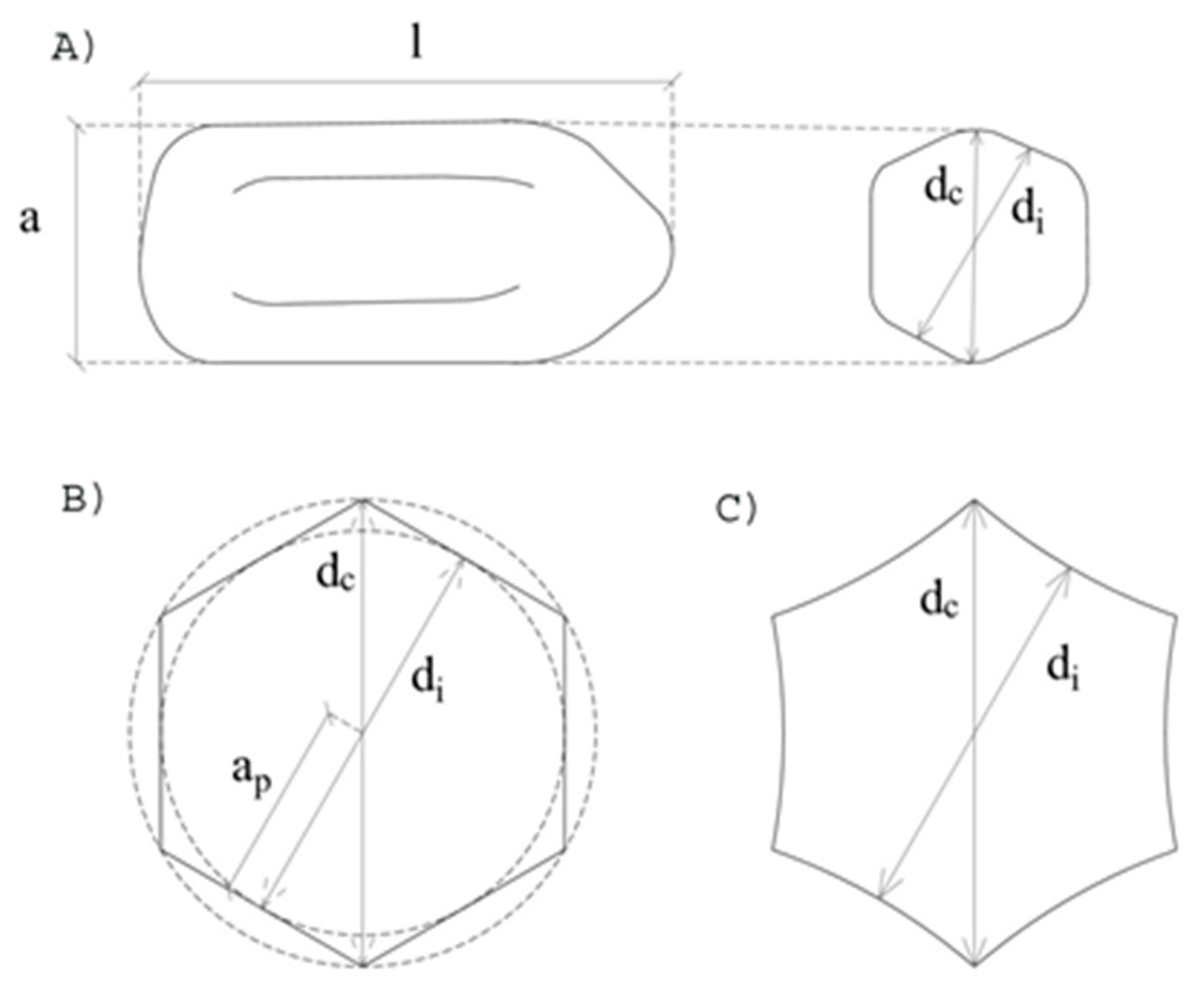
2.2. Morphological Characterization

Detritic elements of termites nesting in wood are hexagonal and prism-shaped, with one or both ends rounded and even pointed, with a slight concavity on the faces (Figure 1). Previous studies showed that both the dimensions and the shape of the prisms vary according to species [10,11,17]. A circle can be circumscribed with diameter d_c, and another circle with diameter d_i can be drawn in a hexagon. In this work, ratio R = d_c/d_i was defined as the geometric parameter of a detritus cross-section shape (Figure 1B). This ratio R in a regular hexagon is equal to 1.15, but in practice, the detritus has a nonregular polygonal shape due to face concavity, and therefore, the ratio R has slightly different values. This parameter was used here to differentiate species.

Ten batches of detritus were selected for each sample, in which 24 detritic elements were randomly measured per batch; 240 elements per sample. In 200 elements, length and width (top view) were measured, and in the remaining 40, the dimensions of the hexagonal cross-section (profile) were also measured. The measurements can be seen in Figure 1, where the shape (top view and cross-section) and measurements are schematically shown. The maximal length (l) and width (a) in micrometers were measured in the top view. The three diagonals between opposite vertices (d_c) and the three distances between opposite faces (d_i) were measured in micrometers in the hexagonal (cross-section) profile. Since diametric measurements are much more complex, fewer elements were measured than was the case for length, although they were always sufficiently representative.

The measurements, which were carried out randomly and covered average sizes as far as possible, excluded elements that were much larger or smaller than the norm. This is because experience shows that the practice of using extreme data can result in an identification error. In this work, the maximal threshold values used for developing the mathematical model were 1100 × 780 micrometers for C. brevis, and 1090 × 620 micrometers for K. flavicollis. The minimal threshold values were 650 × 330 micrometers for C. brevis, and 450 × 300 micrometers for K. flavicollis.

With the obtained dimensional data, fundamental statistical analysis was performed to obtain means and coefficients of variation, and ANOVA with a confidence level of 99% was used to determine the statistical differences between groups of origin and species.

Morphological analysis was also performed on the qualitative variability of the observed shapes: more rounded or more pointed ends, variations in symmetry, or the presence of elements other than pellets (for example, detritic elements and wood chips). Color differences were verified by groups or within the same sample. To simplify the process, only light, dark, homogeneous, and heterogeneous colors were distinguished. The age of the attack, the wood species, and its pathological condition influence the color of the detritus, and these factors must be taken into account.

A Comecta Ivymen System stereo microscope was used for dimensional, shape, and color analysis. This device incorporated a 3-megapixel Moticam 2300 digital camera with a USB 2.0 connection and analysis software Kopa Cam 5.4 that measures with micrometer precision.

2.3. Prediction Models

Discriminant statistical analysis was carried out to identify the type of termite.

The classification functions had the form of Equation (1), where YSp is the result for each species of the model; X and Z are the coefficients that multiplied the used dimensional variables; V1 and V2 are the dimensional variables of the model; and C is a constant.

YSp = X × V1 + Z × V2 + C.

(1)

Each analyzed species provided a classification function (with different coefficients X and Z, and constant, C). If the new measured dimensional values were introduced into these functions, the equation with the highest result corresponded to the most probable species.

Finally, the proposed models were tested with another sample of detritic elements from the same population; six origins were selected at random, three from each species and origin. Length and width were measured in twelve new elements, and diameter was measured in four elements, with a total of 72 measurements of the top view (1 × a) and 24 measurements of the cross-section (d_c × d_i).

3. Results and Discussion

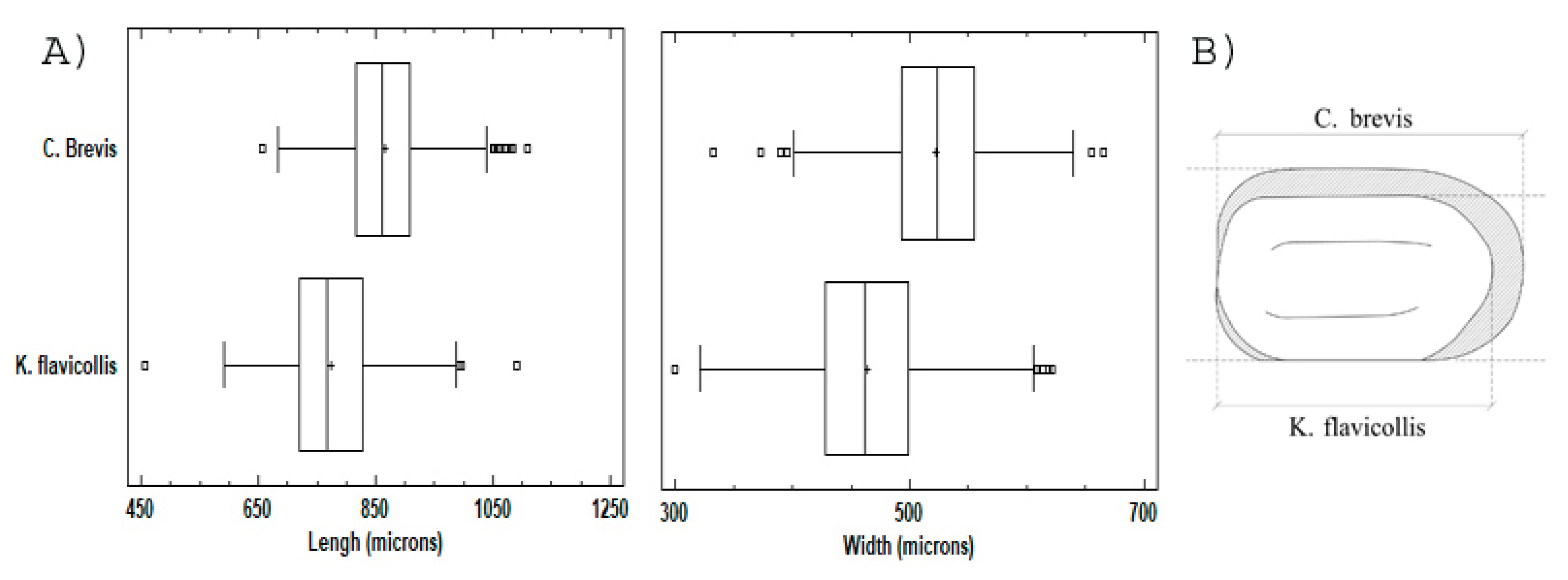
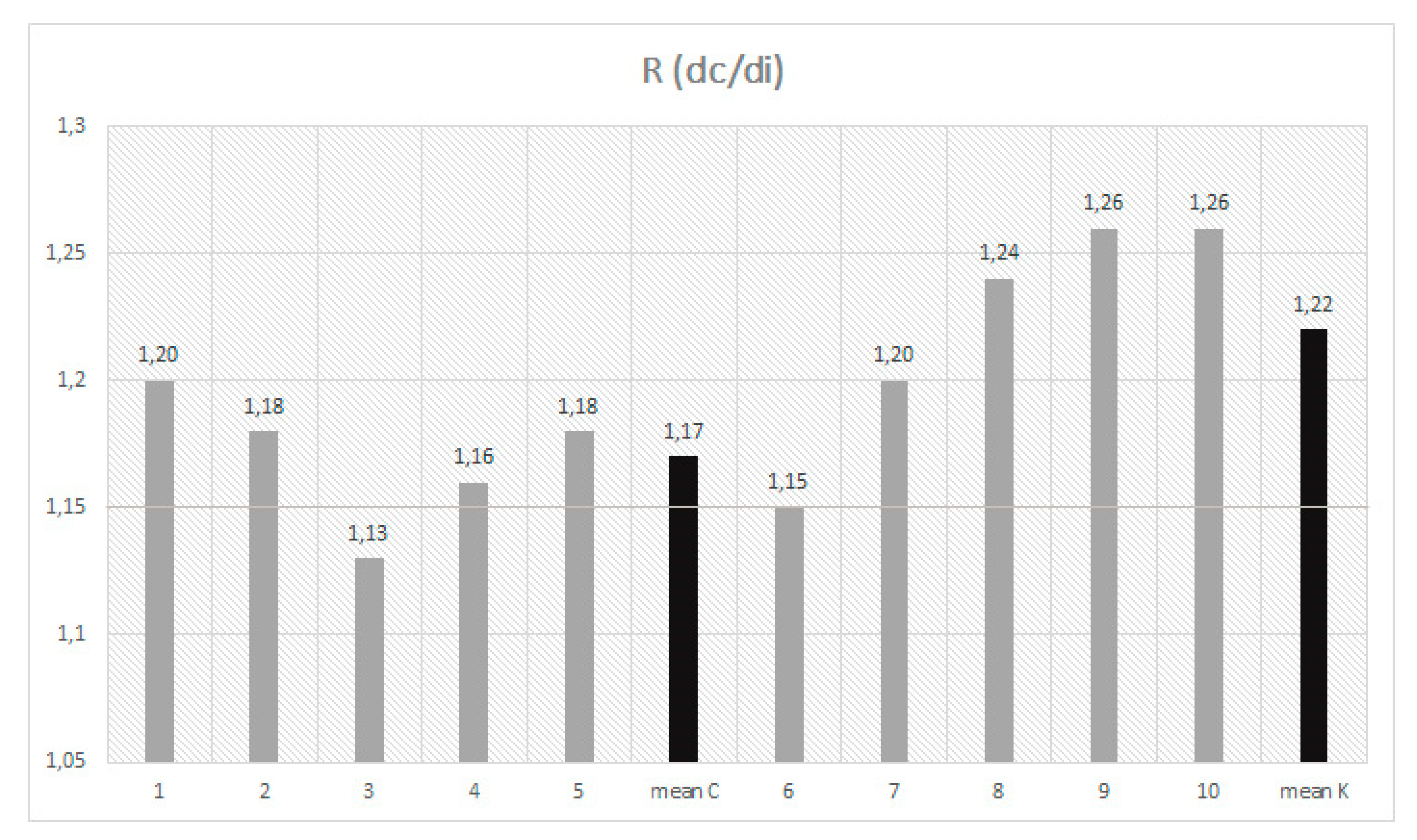
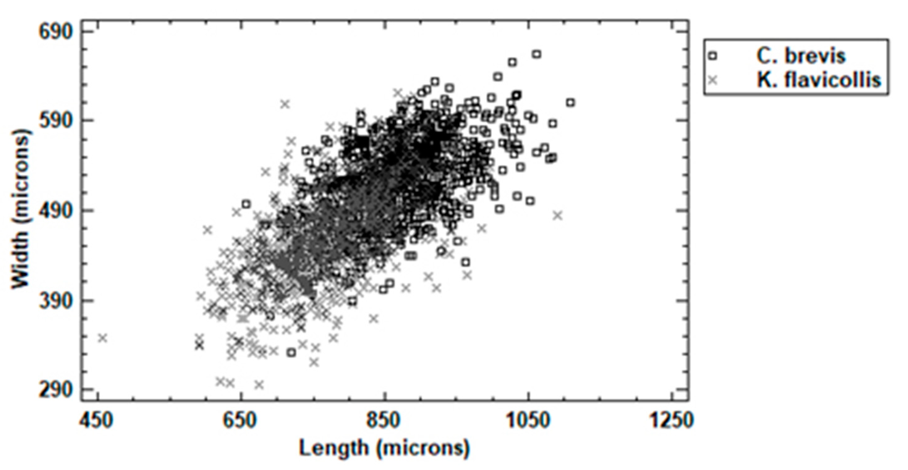
3.1. Dimensional Analysis

Table 2. Results of dimensional termite-detritus analysis. Average values by groups and by species. Statistical differences between groups of origin (lowercase letters) and species (uppercase letters) using ANOVA test with a confidence level of 99% are also shown. Different letters indicate statistical differences.

Sample	Sp.	l (µm)	CV (%)	SE (%)	a (µm)	CV (%)	SE (%)	dc (µm)	CV (%)	SE (%)	di (µm)	CV (%)	SE (%)	R (dc/di)	CV (%)	SE (%)
1	Cb	867 z	6.7	4.1	524 z	6.7	2.5	523 z	5.8	4.8	438 z	7.9	5.4	1.20 z	4.1	0.008
2		933 y	7.1	4.7	555 y	6.8	2.7	550 y	9.5	9.5	466 y	10.2	8.7	1.18 zy	4.2	0.009
3		867 z	5.4	3.3	536 x	6.7	2.5	537 zy	6.9	5.9	475 y	6.6	5.0	1.13 x	3.5	0.006
4		816 x	6.6	3.8	501 w	8.9	3.2	492 x	10.5	8.2	424 z	10.7	7.3	1.16 y	3.6	0.007
5		843 w	7.6	4.6	495 w	8.8	3.1	498 x	9.1	7.1	423 z	11	7.3	1.18 z	3.8	0.007
Mean		865 Z	8.1	2.2	522 Z	8.7	1.4	518 Z	9.3	3.5	444 Z	10.4	3.4	1.17 Z	4.3	0.004
6	Kf	813 xv	9.4	5.4	524 z	8.4	3.1	526 z	9.6	9.2	459 y	11.1	9.3	1.15 yx	3.3	0.007
7		801 v	9.1	5.2	481 v	8.1	2.8	467 w	8.8	6.2	389 x	10.3	6.0	1.2 z	3.7	0.007
8		731 u	8.6	4.5	435 u	7.8	2.4	433 v	6.9	5.2	351 w	7.1	4.4	1.24 w	4.8	0.010
9		773 t	12.1	6.6	437 ut	12.9	4.0	402 u	16.4	11.7	323 v	20.4	11.6	1.26 w	6.2	0.014
10		754 s	7.8	4.1	445 t	9.3	2.9	375 t	15.8	9.3	300 u	19.4	9.1	1.26 w	6.3	0.012
Mean		774 Y	10.3	2.5	464 Y	11.9	1.7	438 Y	16.4	5.4	362 Y	20.3	5.5	1.22 Y	6	0.005

Sp: species; Cb: C. brevis; Kf: K. flavícolis; l: length; a: width; dc: circumscribed diameter; di: inscribed diameter; R: concavity factor; CV: coefficient of variation; SE: standard error.

shows the average results of dimensional analysis, length, width, diameters, and R ratio of concavity. The statistical differences between the groups (different lowercase letters) and the two species (different uppercase letters) are also shown. In all groups, normality was verified before variance analysis.

Detailed analysis of the results of Table 2 showed significant statistical differences in average dimensions according to species, as they were smaller in the groups of K. flavicollis, at 10.5% shorter in length and 11.1% smaller in width. Although this is a surprising result since individuals of this species are larger than those of C. brevis, it agreed with the obtained results in previous exploratory work [10,11].

Figure 2 statistically (A) and graphically (B) shows the difference in average size between species. Measurements of the detritic elements of K. flavicollis were more variable (with higher coefficients of variation), according to species and within each group of origin, Table 2. This may be due to the greater variety of sizes of the individuals in the analyzed K. flavicollis colonies, and this also depends on the maturity of the colony. This should be taken into account when making measurements for classification while avoiding outlier measurements.

Statistical differences between the two species in length and width were found and were very useful for identification (Table 2). Figure 2A shows these differences in the form of a box and whisker chart.

Clear statistical differences between species were also observed in concavity factor R, although in this case, the groups of each species were more homogeneous (Table 2). Practically, almost all groups measured in both species had a concavity (R values higher than 1.15), but this was more pronounced in K. flavicollis, with an average factor of 1.22 compared to 1.17 in C. brevis (Figure 3). This morphological differentiation was also observed in previous works [10], and it could be observed by the naked eye in a good part of the analyzed samples. The cause of this greater curvature in the faces of the hexagon is unknown. However, the different humidity levels of the colonies, low in those of C. brevis and high in those of K. flavicollis, may play an important role since detritic elements are cellulose derivatives that have hygroscopic properties. Therefore, if detritic K. flavicollis elements started from a more humid initial state, there would be more significant decrease and deformation.

The higher variability in the results of cross-section dimension measurements (diameters) in comparison to those of the top view (length and width) is evident. In the former, coefficients of variation were considerably higher (Table 2). This was due, on the one hand, to the greater difficulty involved in performing this measurement, which may therefore have given rise to more significant human error. On the other hand, it was also because the shape of the detritic elements was more variable than their overall dimensions, so that it was not infrequent to find elements of different widths and concavities with equal lengths in the same sample.

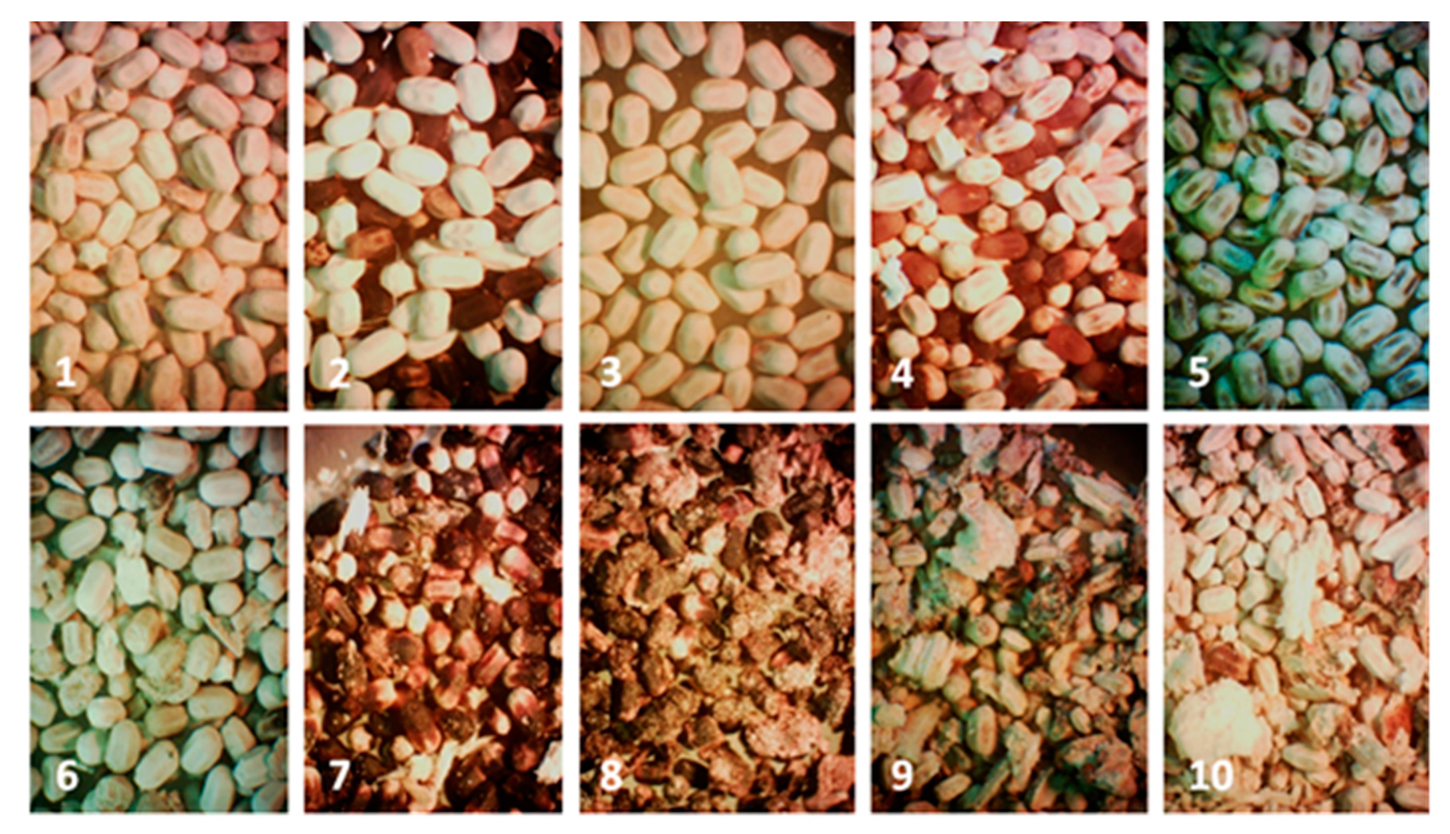
3.2. Shape and Color Analysis (Aspect)

If the debris as a whole were observed, and focusing first on the top view (Figure 1), we found a certain degree of morphological variability. It was possible to see more or less elongated elements, with one or both ends tapered, or like a pencil shape where one end was rounded and the other was tapered. The width of the prism was not always regular, and there were sometimes marked differences between one end and the other. Differences in the concavity on the faces of the cross-section could be observed: some elements had flat faces, while others had varying degrees of curvature.

The colors were also quite variable, with elements that were light beige, light to dark brown, and even black. The same sample could have varied colors, and there was even variation between zones of the same element.

Unlike the objective measurements of the previous section, morphological and color analysis did not sufficiently differentiate the two species. Nevertheless, a visual element generally did allow this: the presence of wood remains without any definite shape or color in K. flavicollis samples that had a “dirtier” appearance (Figure 4). The presence of these remains next to the detritic elements was due to the pathological state of the wood, which generally showed a fungal attack and therefore greater disintegration of the woody tissue.

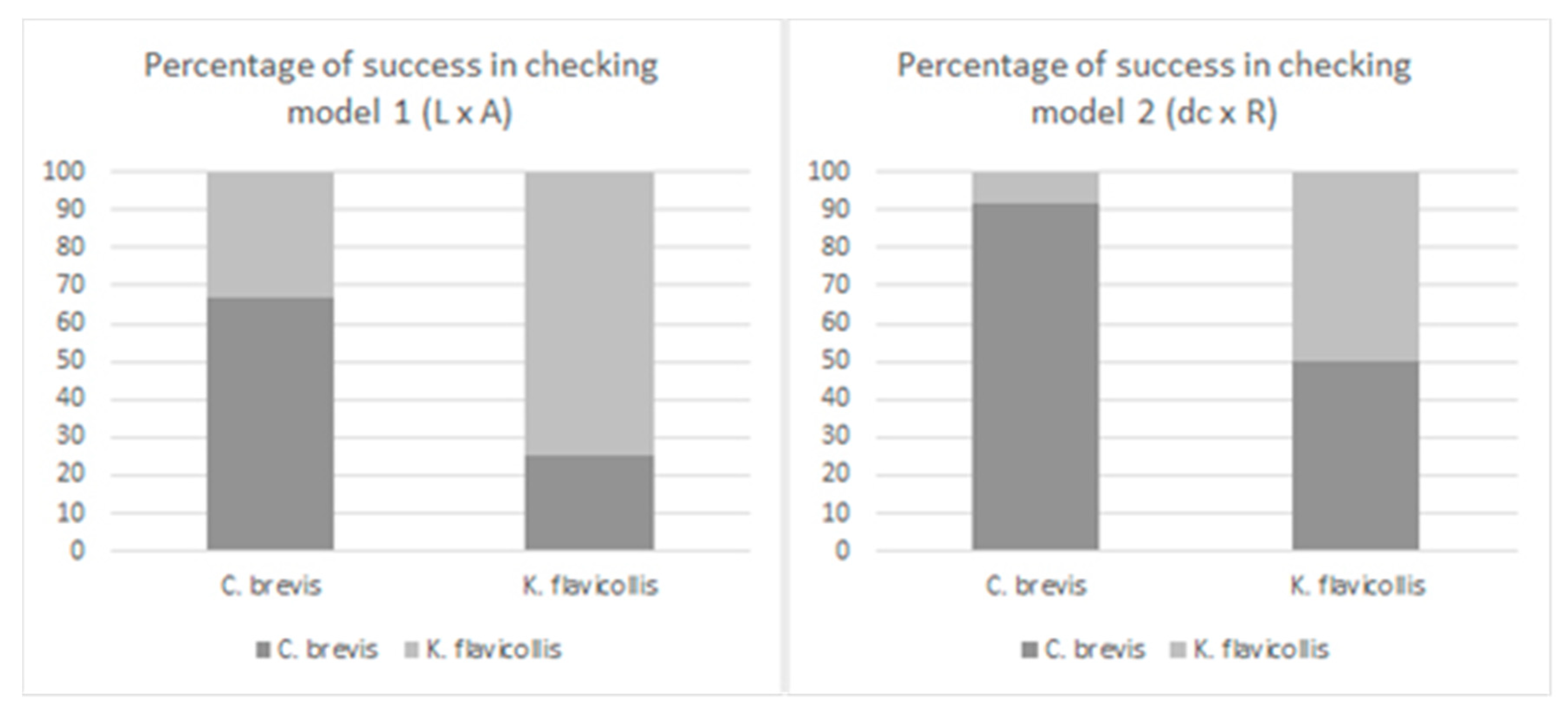
3.3. Prediction Models

Since the results of the dimensional section showed apparent differences between the species in top-view dimensions (length and width) and in the degree of concavity of the hexagonal cross-section of the detritic elements, discriminant statistical analysis would be an objective and simple tool for the identification of the type of termite. First, discriminant analysis (Model 1) was carried out using top-view measurements (length and width), which were faster and easier to use. As can be seen in Figure 5, dispersion of the pairs of values clearly showed the differentiation between the two species. However, there was an important degree of overlap that always gave rise to particular uncertainty. In this model, the predictive functions gave a success rate of 75.2%. Analysis was then repeated using the circumscribed diameter (d_c) and the concavity R factor (d_c/d_i) (Model 2) as dimensional variables. In this case, differentiation was slightly better (Figure 6), and the success rate was 76.9%. This slight improvement of the results in Model 2 was, however, negligible if we take into account that these measurements were far more difficult.

Predictive results were more modest than those found by Recarte [10], which is explained by the number of samples, their origins, and their variability, which were all much higher in this work.

Table 3. Coefficients and constants of classification functions according to species. Model 1 corresponds to length- and width-based functions, and Model 2 corresponds to circumscribed-diameter- and concavity R factor-based functions. Assigned percentage of success shown in first column next to the model.

	Dimensional Variable	C. brevis	K. flavicolis
Model 1 (75.19%)	Length (L)	0.111221	0.100192
	Width (W)	0.110188	0.096958
	Constant (C1)	−77.5688	−62.0013
Model 2 (76.90%)	Circumscribed Diameter (dc)	0.334091	0.314628
	R factor (dc/di)	433.907	438.855
	Constant (C2)	−341.057	−337.666

shows all variables of the classification functions, with the length and width (Model 1), and with the circumscribed diameter and the R factor (Model 2), according to Equation (1). More sophisticated models with all four variables were tested without any improvement in the prediction results.

The obtained verification results in Figure 7 showed that the average success rates were higher than 70%. Moreover, all samples were correctly classified when considering the average of the measurements, and not just the individual measurements of the elements. The overall behavior of the two models was similar, although Model 2 worked better with C. brevis than it did with K. flavicollis. Therefore, Model 1 was preferable, since the results were more balanced and similar for both species.

4. Conclusions

The dimensions of the detritic elements, both in the top view and cross-section, were larger in Cryptotermes brevis. Kalotermes flavicollis had a greater concavity on the faces of the hexagonal cross-section (R factor). Both factors presented significant statistical differences.

Two statistical prediction models were proposed on the basis of these detected differences. These models had a success rate of over 75% in both cases, and they were tested using new measurements with satisfactory results.

Kalotermes flavicollis samples always looked “dirtier” since detritic elements appeared accompanied by wooden residues due to the pathological state of the attacked wood. This factor could also be taken into account when differentiating between species.

Given the found variability, it is recommended to measure a sufficient number of detritic elements when using the prediction models, and checking all individual measurements and mean values to avoid the influence of outliers. It is also recommended to make a random selection of representative detritic elements during measurements, avoiding extreme cases as far as possible (very large or tiny dimensions). If doubtful results are obtained, consideration of the visual aspect of the sample is added to dimensional analysis.

This paper raises new questions to investigate in the future. The first has to do with the relationship between the size of the individuals of a species and the size of the detritic elements that they produce, which had an inverse rati in this work o. The second question is on the dimensional variability of the debris and how it evolves with the maturity of a colony.

References

1. Benito, M.J. El termes de madera seca (Cryptotermes brevis) en las islas Canarias. Serv. Plagas For. Rev. Montes 1957, 75, 147–161. [Google Scholar]
2. Benito, M.J. Los termitos en España. Biología, daños y métodos para combatir la especie subterránea Reticulitermes lucífugus. In Servicio de Plagas Forestales. Serie B, nº 6; Dirección General de Montes, Caza y Pesca fluvial: Ministerio de Agricultura, Spain, 1958; p. 23. [Google Scholar]
3. Becker, G.; Kny, U. Survival and development of the drywood termite Cryptotermes brevis (Walker) in Berlin. Anz. Schadl. Pflanz. 1977, 50, 177–179. [Google Scholar]
4. Rainieri, V.; Rey, A.; Marini, M.; Zafaggnini, V. A new discovery of Cryptotermes brevis in Genoa, Italy (Isoptera). Boll. Soc. Entomol. Italiana. 2001, 133, 99–102. [Google Scholar]
5. Nunes, L.; Gaju, M.; Krecek, J.; Molero, R.; Ferreira, M.; De Roca, C.B. First records of urban invasive Cryptotermes brevis (Isoptera: Kalotermitidae) in continental Spain and Portugal. J. Appl. Entomol. 2010, 134, 637–640. [Google Scholar] [CrossRef]
6. Guerreiro, O.; Cardoso, P.M.; Ferreira, J.M.F.; Ferreira, M.T.; Borges, P.A.V. Potential distribution and cost estimation of the damage caused by Cryptotermes brevis (isóptera: Kalotermitidae) in the Azores. J. Econ. Entomol. 2014, 107, 1554–1562. [Google Scholar] [CrossRef] [PubMed] [Green Version]
7. Evans, T.A.; Forschler, B.T.; Kenneth Grace, J. Biology of invasive termites: A worldwide review. Annu. Rev. Entomol. 2012, 58, 455–474. [Google Scholar] [CrossRef] [PubMed] [Green Version]
8. Barco Villalba, N. Análisis de las Características Morfológicas y Anatómicas del Detrito, Galerías y Larvas de Hylotrupes Bajulus L. y su Evolución en Condiciones Controladas de Laboratorio; TFC EUITF For.-UPM. Director: Madrid, Spain, 2010; p. 58. [Google Scholar]
9. Bobadilla, I.; Arriaga, F.; Luengo, E.; Martínez, R. Dimensional and morphological analysis of the detritus from six European wood boring insects. Maderas Cienc. Tecnol. 2015, 17, 893–904. [Google Scholar] [CrossRef] [Green Version]
10. Recarte Gallego, J. Diferenciación de las Especies de Termitas Cryptotermes brevis (Walker, 1853) y Kalotermes flavicollis (Fabricius, 1793) Mediante el Análisis Morfológico y Dimensional de sus Detritos; TFC ETSI de Montes, Forestal y del Medio Natural-UPM. Dir: Madrid, Spain, 2017; p. 47. [Google Scholar]
11. Rivera Rubio, M. Análisis Morfológico y Dimensional del Detritus de las Especies de Insectos Xilófagos más Frecuentes en la Madera Estructural; TFC ETSI de Montes, Forestal y del Medio Natural-UPM. Dir: Madrid, Spain, 2017; p. 90. [Google Scholar]
12. Rodriguez Barreal, J.A. Patología de la Madera; ETSI de Montes, Ed.; FUCOVASA-Mundiprensa: Madrid, Spain, 1998; p. 349. [Google Scholar]
13. Arriaga, F.; Peraza, F.; Esteban, M.; Bobadilla, I.; García, F. Intervención en Estructuras de Madera; Aitim: Madrid, Spain, 2002; p. 476. [Google Scholar]
14. Hay, C.J. Frass of some wood boring insects in living oak. Ann. Entomol. Soc. Am. 1968, 61, 225–258. [Google Scholar] [CrossRef]
15. Oevering, P.; Pitman, A.J. Characteristics of attack of coastal timbres by Pselactus sapadix Herbst and an investigation of its life history. Holzforschung 2002, 56, 335–359. [Google Scholar] [CrossRef]
16. Haverty, M.; Woodrow, J.; Nelson, l.; Grace, K. Identification of termite species by the hydrocarbons in their faeces. J. Chem. Ecol. 2005, 31. [Google Scholar] [CrossRef] [Green Version]
17. Hickin Norman, E.; Edwards, R. The Insect Factor in Wood Decay: An Account of Wood Boring Snsects with Particular Reference to Timber Indoors; Hutchinson and Co. Publishers Ltd.: London, UK, 1975; p. 383. [Google Scholar]
Figure 1. Shape of detritic elements. A) Top view and cross-section, detail of measurements, length (l) and width (a) with circumscribed and inscribed diameters (dc and di); B) measurement in regular hexagon; and C) face concavity.
Forests 11 00408 g001
Figure 2. (A) Box and whisker chart for length and width of detritic elements of two species, C. brevis and K. flavicollis. (B) Comparative drawing to scale with average dimensions of each species.
Forests 11 00408 g002
Figure 3. Concavity factor R. Groups 1 to 5 correspond to C. brevis, and Groups 6 to 10 correspond to K. flavicollis. Line 1.15 corresponds to null concavity of regular hexagon.
Forests 11 00408 g003
Figure 4. Detritic elements of analyzed samples. Images 1 to 5 correspond to C. brevis; images 6 to 10 correspond to K. flavicollis. Shape and color of detritic elements were very similar in both species. However, the “dirtier” debris appearance in images 6 to 10 can be clearly seen. Wood residues of variable appearance and shape could be found together with detritic elements.
Forests 11 00408 g004
Figure 5. Scatter diagram of length and width data pairs of measured detritic elements.
Forests 11 00408 g005
Figure 6. Scatter diagram of circumscribed diameter and R factor pairs of measured detritic elements.
Forests 11 00408 g006
Figure 7. Comparison of test results of statistical models with new measurements. Bars show 10–20 elements for top view, and 4–8 elements for cross-section, as samples could be quite variable.
Forests 11 00408 g007