Article

Patterns of Density and Production in the Community Forests of the Sierra Madre Occidental, Mexico

by
Jaime Roberto Padilla-Martínez
1,
José Javier Corral-Rivas
1,*,
Jaime Briseño-Reyes
1,
Carola Paul
2,
Pablito Marcelo López-Serrano
3 and
Klaus v. Gadow
4,5,6
1
Facultad de Ciencias Forestales, Universidad Juárez del Estado de Durango, Río Papaloapan y Boulevard Durango, Durango 34120, Mexico
2
Forest Economics and Sustainable Land-use Planning, Georg-August-Universität, Büsgenweg 5, 37077 Göttingen, Germany
3
Instituto de Silvicultura e Industria de la Madera, Universidad Juárez del Estado de Durango, Boulevard del Guadiana 501, Durango 34120, Mexico
4
Faculty of Forestry and Forest Ecology, Georg-August-Universität, Büsgenweg 5, 37077 Göttingen, Germany
5
Department of Forestry and Wood Science, Faculty of AgriSciences, Stellenbosch University, Stellenbosch Private Bag X1, Matieland 7602, South Africa
6
Department of Ecology, Beijing Forestry University, Tsinghua East Road 35, Beijing 100083, China
*
Author to whom correspondence should be addressed.
Forests 2020, 11(3), 307; https://doi.org/10.3390/f11030307
Submission received: 26 January 2020 / Revised: 5 March 2020 / Accepted: 8 March 2020 / Published: 11 March 2020
(This article belongs to the Section Forest Ecology and Management)

Abstract

:
The Mexican Sierra Madre Occidental (SMO) represents a region where hundreds of plant species reach the limits of their northern or southern range. The SMO also features a unique cultural diversity, and many communities living within the forest or in its close vicinity depend on the products and services that these forests provide. Our study was based on a large set of remeasured field plots placed in the forests of Durango which are part of the SMO. Using hierarchical clustering, three distinctly different forest types were identified based on structural differences and the relation between stem density and basal area. Maximum forest densities were estimated using a 0.975th quantile regression. Forest production (expressed as current periodic volume increment per unit of area and time) was estimated based on number of stems, forest density, mean height, and forest diversity. Forest density is the principal factors affecting periodic volume production. The discussion presented recommendations for the sustainable use of this unique natural resource. Maintaining minimum levels of residual density is key to ensuring the continued viability of the forests of the Mexican SMO. Future research is needed to identify optimum residual structures, productive residual densities, and desirable levels of biodiversity.

1. Introduction

Forest density is a multifaceted phenomenon, and the terminology relating to forest density is often the cause of misunderstanding. To prevent imprecise and confusing usage of the term, there is a need for clarification. In this study, we defined forest density as the degree of site occupancy by trees, i.e., the total tree biomass per unit forest area. It is almost impossible to assess that quantity. Therefore, basal area (the sum of the cross-sectional areas of the trees at breast height) is often used as a practical substitute for biomass. Forest density can be expressed in absolute or relative terms. Absolute measures of density are determined directly for a given location. Relative density is used to compare a given density with some standard, such as the full stocking of a yield table [1,2].
Observations about maximum forest density may provide a basis for environmental gradient analysis, for example in addressing the question: Which are the site conditions that most affect the potential density of a forest ecosystem? Knowledge of maximum forest density permits comparisons of potential biomass and carbon estimates with observed values. The ability to predict maximum forest density also enables foresters to quantify the reduction of biomass and the loss in carbon sequestration by timber harvesting. This will permit more accurate and comprehensive comparisons of different residual structures for forest management [3].
Some studies have revealed interesting and rather large differences in maximum density for different tree species on the same site and for the same species on different sites [4]. As a consequence, to characterize density, forest scientists pioneered more sophisticated approaches than the simple number of organisms commonly used in other branches of ecology. To measure density, the number of trees must thus be qualified by their size [2,5]. For those reasons, density management studies in mixed stands should be focus on all species present and include the interspecific and intraspecific competition effects [6]. West [7] compared 17 different measures of site occupancy by trees. The most common measures were basal area, leaf area index, stand density index, Nilson’s sparsity, relative spacing, and crown competition factor.
Equally multifaceted is the term ‘forest structure,’ which refers to the way in which the attributes of trees (species, size, position) are distributed within a forest community. The production and dispersal of seeds and the associated processes of germination, seedling establishment, and survival are important factors of plant population structuring [8]. The empirical diameter distribution is an important attribute of a forest community and widely used for characterizing forest structure [9]. The distribution of the tree diameter at breast height (dbh; cm), frequently used as an input for forest growth models, enables economic assessment of timber value and the development of management schedules [10]. Because of its flexibility and ability to describe a wide range of unimodal distributions, the Weibull function is a preferred model [11,12,13].
Knowledge of the productive potential of a forest ecosystem is also essential for its sustainable use. In this study, forest production was defined as the periodic volume increment per unit area and time. Stand density represents essential information for assessing site productivity, modelling and predicting stand dynamics, and silvicultural management [14]. Studies involving the relationship between density and production, usually based on long-term observation periods, are particularly challenging in mixed multi-aged stands, where the selection of appropriate residual densities requires practical guidance [15,16].
The Sierra Madre Occidental (SMO) is the largest mountain range in Mexico and is characterized by a unique social and cultural diversity of the inhabitants who are living within the forest or in its close vicinity [16]. These forests have a high species richness with three physiognomically dominant genera: 24 species of Pinus (46% of the Mexican total), 54 species of Quercus (34%), and 7 species of Arbutus (100%). The SMO that includes the forest of Durango state represents a boundary area where hundreds of species reach their northern or southern range limits. It also contains numerous endemic elements [17,18]. Thus, this region provides an excellent opportunity for improving estimates of the potential density and forest production of mixed multi-aged forests.
Forest density measured by various indices may provide a basis for rational management of the SMO forests. The definition of optimal residual basal area is especially important for different groups of stands. Thus, the objectives of this study were to: (i) Test the suitability of grouping plots based on similarities in structural characteristics; (ii) estimate maximum and optimal forest densities; and (iii) evaluate the effects of density, species diversity, and site quality on forest production.

2. Materials and Methods

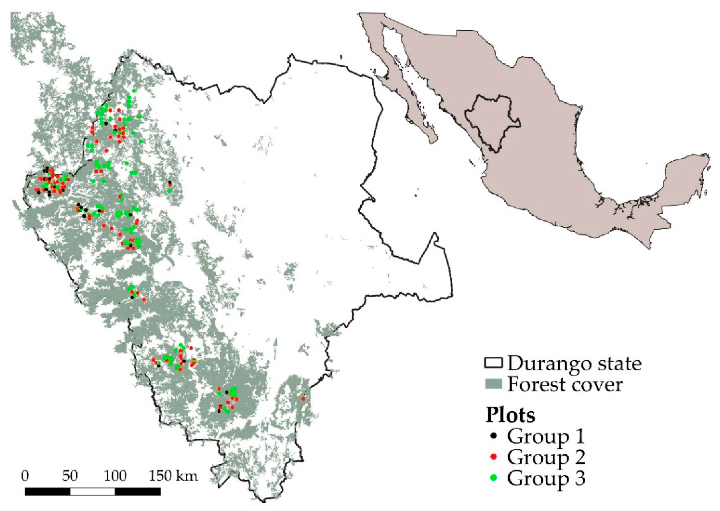
2.1. Permanent Field Plots

The observations used in this study were obtained from a network of permanent sample plots that are used to monitor the dynamics of the forests of Durango [19]. Altogether, 217 undisturbed plots without intermediate harvesting between remeasurements were selected for this study. A summary of the plots is presented in Table 1 for the two inventories.
The plot establishment began in 2007, and remeasurements started in 2012. Each plot was remeasured after five years. The research plots included the main types of the forest stands in the SMO, providing an opportunity to study patterns of forest structure, density and production in this unique socioecological region. Each plot covered an area of 50 m × 50 m. The plots were distributed systematically, with a variable grid ranging from 3 km to 5 km depending on the size of the land properties. The tree number, species, dbh, total tree height (h; m), height to the live crown (hc; m), azimuth (A; degrees), and distance (d; m) from the center of the plot of all trees equal or greater than 7.5 cm in dbh were recorded.
The forests of the SMO have been managed by local communities for more than 100 years, mainly using selective harvest for sustainable timber production, but also for the maintenance of biological diversity and uneven-aged stand structures. The Continuous Cover Forestry System is preferred in the region because it promotes mixed and irregular forest stands and high biodiversity. It is known as the Mexican Method of Irregular Forest Regulation and is characterized by the absence of a rotation age that defines the time of the harvest. The stand age is undefined because trees of all ages usually occur in close vicinity to each other. Commercial harvests are based on maintaining growing stock levels within an ideal and negative exponential diameter class distribution, which is also known in the literature as an inverse J-shaped distribution. In uneven-aged stands, the idealized diameter distribution is thought to be balanced, meaning that it can be maintained by applying a given harvest rate in perpetuity [16].

2.2. Stratification of Field Plots

The distribution of diameters and heights were estimated by the Weibull model [20] using the function fitdistr of the MASS package [21] of R 3.6.0 [22]. The Weibull individual scale and shape plot parameters estimates were then grouped using the R function hclust [22] to obtain, iteratively and based on the method of centroids, a hierarchical cluster of the parameter estimates [23]. Among the different choices of cluster analysis, the methodology implemented in the hclust function of R, which is based on the complete linkage method for hierarchical clustering, was applied. This method defines the cluster distance between two clusters to be the maximum distance between their individual components. At every stage of the clustering process, the two nearest clusters were merged into a new cluster. The process was repeated until the whole data set was agglomerated into one single cluster.
In addition to careful inspection of the dendrogram classification of clusters, the Kruskal–Wallis Rank Sum Test (a nonparametric equivalent to ANOVA) was used to confirm or reject the results of the cluster process, specifically to test whether the sample plots came from unrelated population, or whether the population distributions were identical without assuming them to follow the normal distribution. The Kruskal–Wallis Rank Sum Test was applied to further discriminate among different groups of field plots, involving the plots for the variables of N, G, Dq, Ho, PAI, and S.
The plots were divided into three groups, which differed in terms of basal area, diameter distribution, and the relationship between number of trees and average tree size (Figure 1). There was no obvious geographical preference. Each of the three groups of plots was widely distributed within the state of Durango, and the groups often mingled at close range.

2.3. Maximum Forest Density

Populations of trees growing at high densities are subject to density-dependent mortality or self-thinning. For a given average tree size, there is a limit to the number of trees per area that may co-exist in an even-aged stand [24]. A self-thinning model was used to describe the allometric relationship between the average tree size and the number of trees per hectare [4,25,26,27]. The limiting relationship was described by the following exponential equation:
ln ( N max ) = ln ( α ) β ×   ln ( Dq )   .
where N m a x is the maximum number of living trees per ha (i.e., the full stocking density level), ln is the natural logarithm, Dq indicates the quadratic mean diameter (cm), α is an empirical coefficient, and β is the slope of the relationship between lnN and lnDq in fully stocked stands. The maximum density was estimated using the 0.975th quantile [28] of the R function quantreg [29]. In addition, we also calculated the Reineke’s Stand Density Index (SDI) for each plot (using our own empirical exponent 1.536, instead of Reineke’s 1.605). The SDI has been used as a measure of density for predicting forest productivity [30]:
S D I = N × ( D q 25 ) β
where N is the number of individuals per area, Dq is the quadratic mean diameter (cm), and β is the allometric exponent that expresses the relation between tree size and number of trees estimated in Equation (1).

2.4. Forest Diversity

The variety of biodiversity indices is bewildering, and many are viewed with suspicion. Most diversity indices are entropies, not diversities, and their mathematical behavior often does not correspond to our intuitive concept of diversity [31,32,33]. However, there seems to be general agreement among statisticians that numbers equivalent [34], not entropy, should be the diversity measure of choice [35]. The first three Hill numbers depend on the weight that is assigned to rare species: q = 0 refers to species richness where rare species carry the same weight as common ones, q = 1 refers to the exponential of Shannon’s entropy index, and q = 2 to the inverse of Simpson’s concentration index. For example, if q = 1, the Shannon index H = p i × log ( p i ) is used, and the corresponding Hill effective number is N = eH’. Effective Hill numbers, instead of entropies, are used increasingly to characterize the taxonomic, phylogenetic, or functional diversity of a community. Obviously, estimates of Hill numbers are a function of the sampling effort.
Following Leinster and Cobbold [36], we may extend community diversity beyond the naive focus on a simple index. In this study, we used the number of tree species in plot (S) and effective Hill numbers to test the grouping of sites with different tree diversity. Obviously, the diversity of a forest ecosystem is not only characterized by species richness, but also by a set of attributes that portray the significant features of heterogeneity within a specific community [37]. The diversity profile of a forest community may be characterized by a number of attributes, including the distribution of species and sizes of individuals, and by the way in which these attributes are spatially mingled.

2.5. Modelling Forest Production

The assessment of forest production, i.e., the periodic annual volume increment per unit area and time (PAI), is fundamental to sustainable forest use [38]. PAI may decrease if the residual stand density diverges from the optimum [39], which may be caused by unsustainable harvesting [16,40]. Reduced production may also be expected in very dense forests where production may be offset by mortality and increasing competition [41]. To determine the relationship between forest site variables and PAI (defined here as the periodic annual volume increment of all live trees plus ingrowth (m3/ha/year)), we used a stepwise linear regression procedure. This method is useful for determining the relative importance of the independent variables and evaluating the order of importance of the variables [42]. The significance level of 5% was used for the selection of candidate predictive site variables in the model. These predictive variables were the measurements at the beginning of the selected five-year growth period. They included the number of trees per hectare (N), the Reineke’s Stand-density Index (SDI); the mean plot height (Hmean, m), the Hill number as a diversity measure (Hill), the stand quadratic mean diameter (Dq, cm), the total basal area of the plot (G, m2 ha−1), and the stand dominant height (H0, m). These predictive variables, along with their various combinations, were tested separately. Nonsignificant variables at 5% were removed in the modelling process. In addition, the relation of PAI and residual levels of G was studied to evaluate the effect of low forest densities on production in the study area.
Model evaluation is an important part of our analysis. We used the coefficient of determination (R2) and the Residual Standard Error (RSE). In addition, the normality of the distribution of residuals and heteroscedasticity were evaluated using the Shapiro–Wilk test [43] and graphical analysis.

3. Results

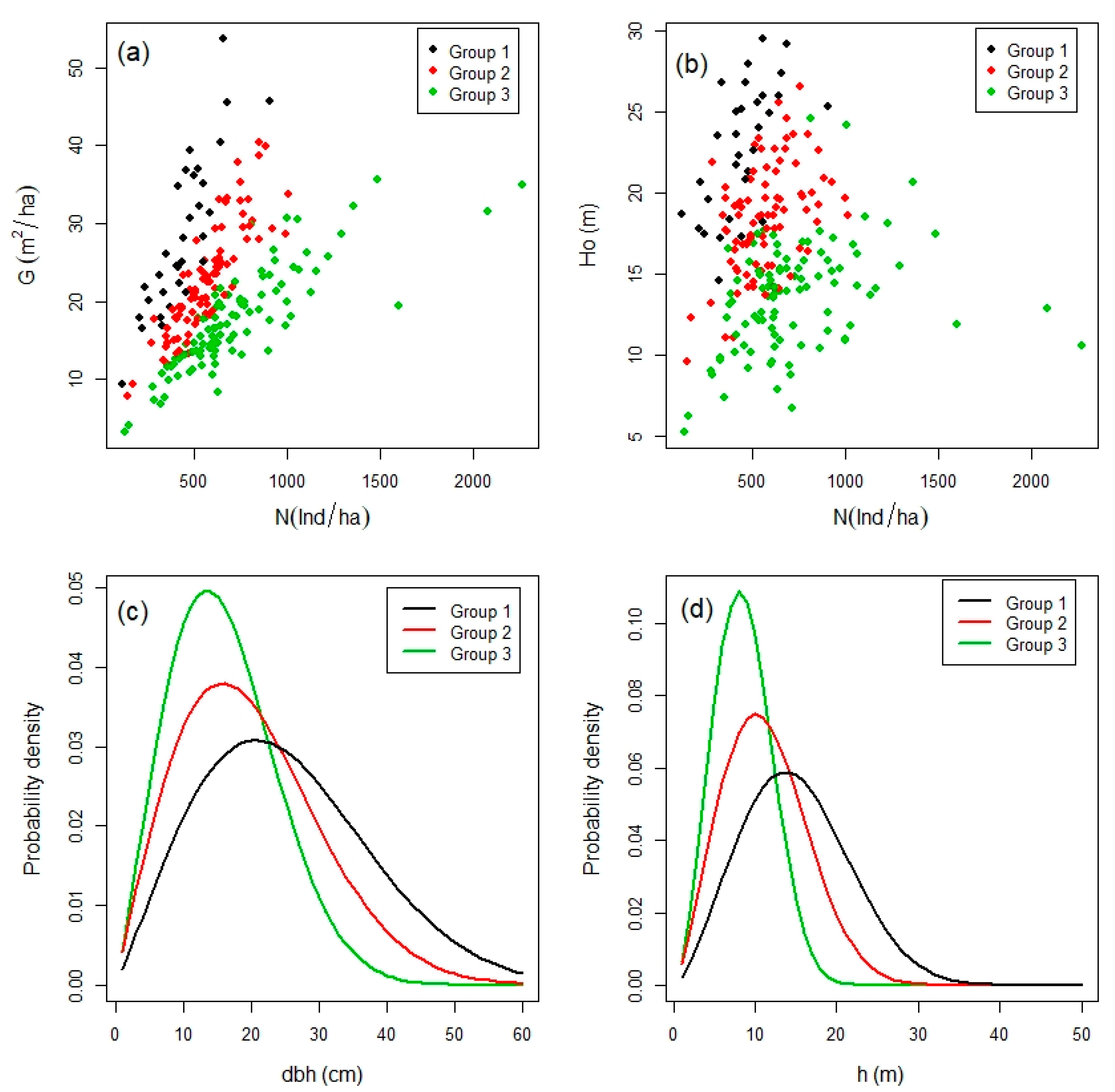
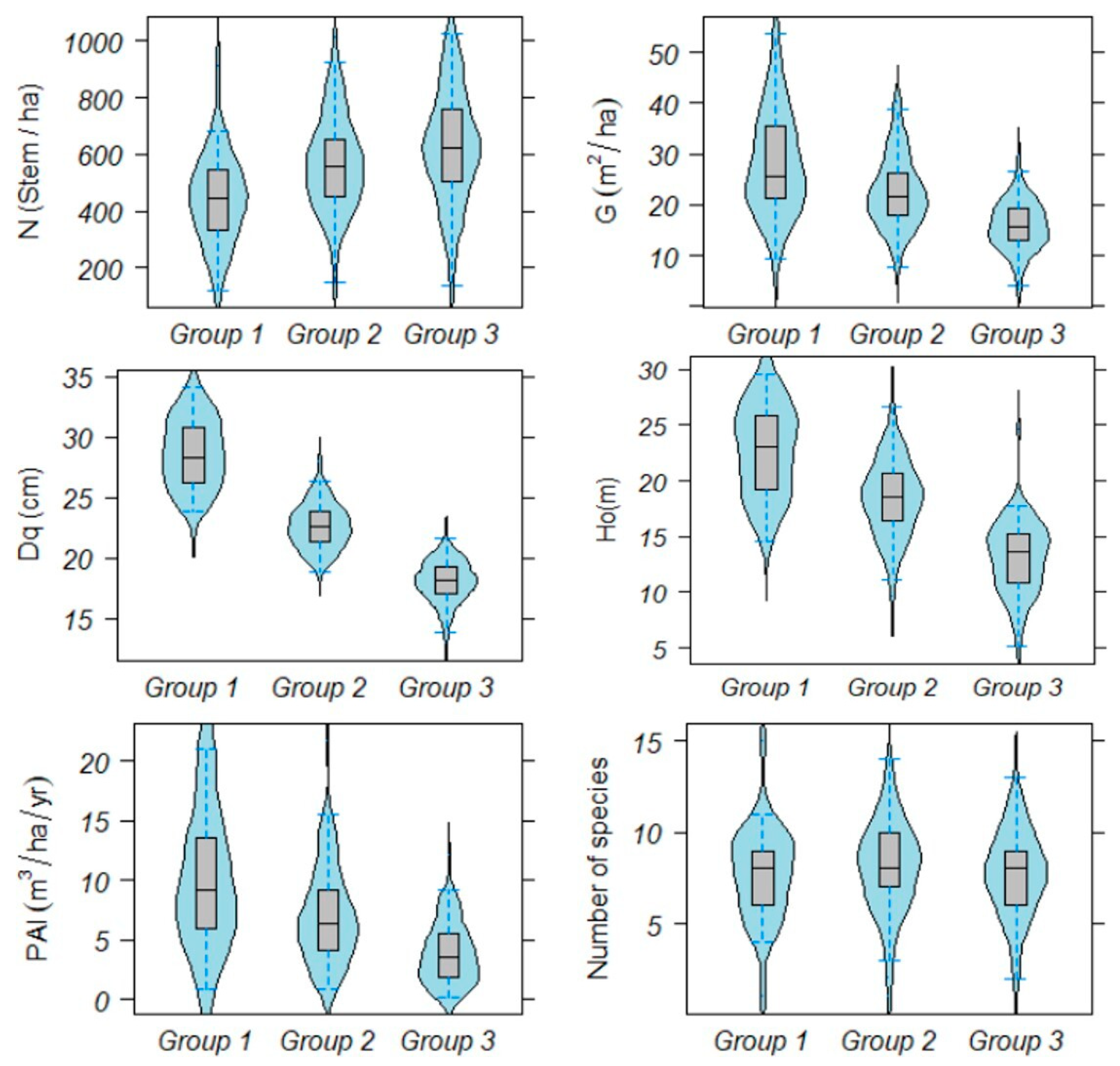
3.1. Stratification of Field Plots

The cluster analysis generated three groups of plots, which described distinctly different forest structures at Sierra Madre Occidental. Figure 2 presents four characteristics of the three groups of plots: (a) The relationship between number of trees and basal area; (b) the relationship between number of trees and dominant height; (c) the diameter distributions; and (d) the height distributions. For the same number of trees (the same "crowding"), forest densities differed greatly among groups. The scale and shape parameters of the Weibull function also differed considerably for diameter at breast height and total tree height.
The results of the Kruskal–Wallis Rank Sum Test, used to further discriminate among the three groups of field plots defined by the cluster process, indicate that the variables N, G, Dq, Ho, and PAI showed highly significant differences (p ≤ 0.01). Only the number of species (S) and Hill number did not show significant differences. This result show that at least one group was distinct from the others. For these cases, we applied Dunn’s test to determine whether all three groups were different or whether only one group was different at the level of 5% (p ≤ 0.05; Figure 3). N, G, Dq, Ho, and PAI suggested significant differences for all of them, indicating that each group corresponded to a significantly different forest structure.

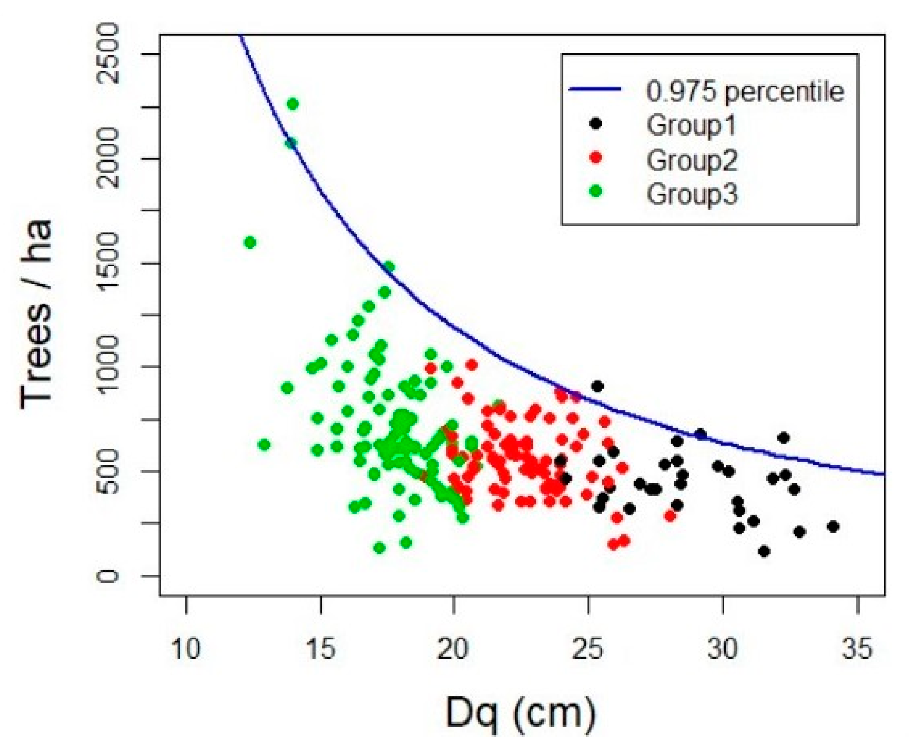
3.2. Maximum Forest Density

The relation between the number of individuals and the basal area, described by Reineke as a site density index that expresses the maximum tree occupancy in each area, was negative in all three density groups (Figure 4). The limiting density estimated for Durango´s forests was ln ( N m a x ) = l n ( 118 , 434.6 ) 1.536 × ln ( D q ) .
The three groups differed from each other in stand density and squared diameter. The highest stand density was observed in Group 3, while the lowest was recorded in Group 1. The squared diameter showed the opposite pattern. Dunn’s test shows significant differences (P ≤ 0.01) among the three groups of plots (Figure 3).

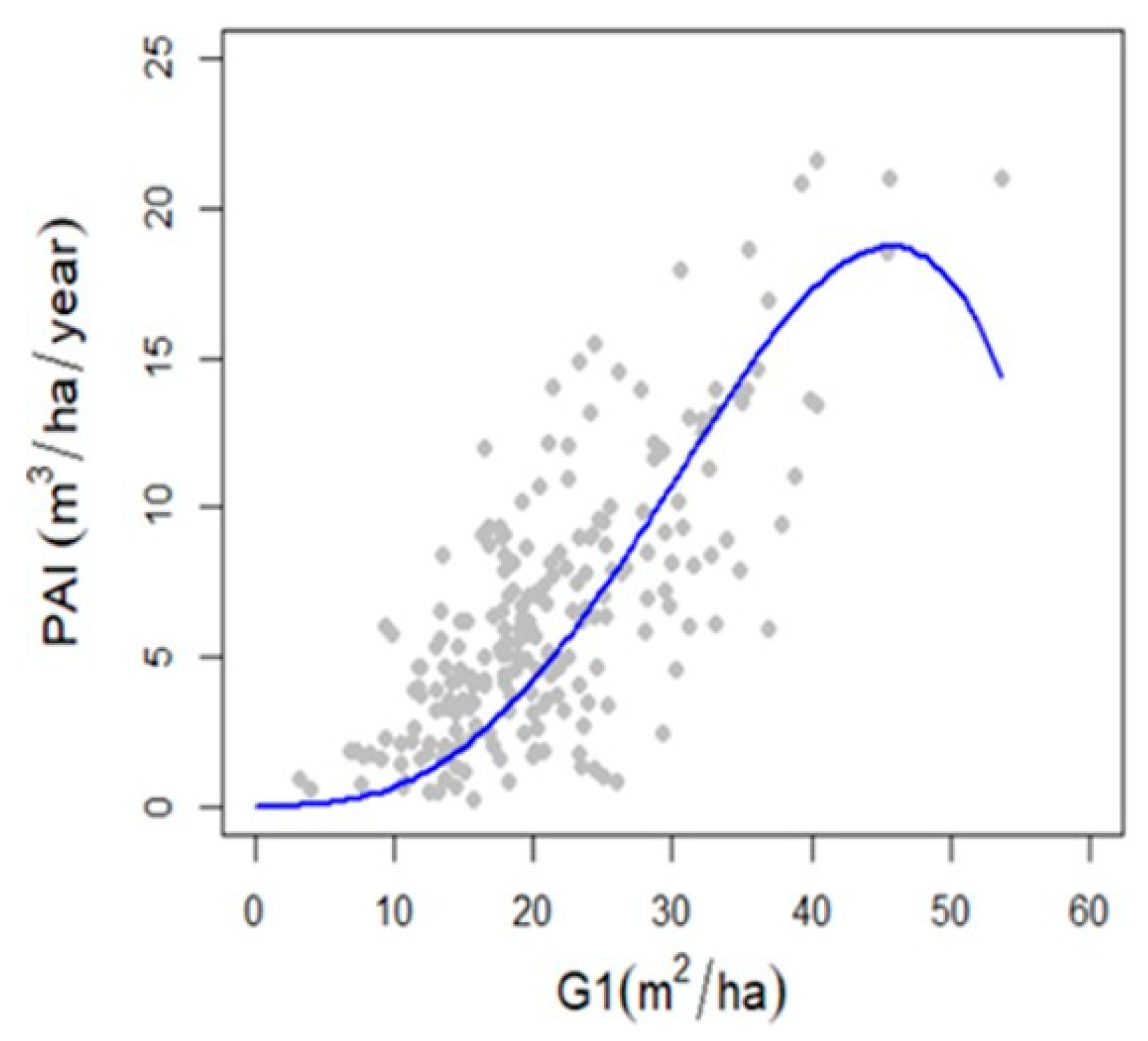
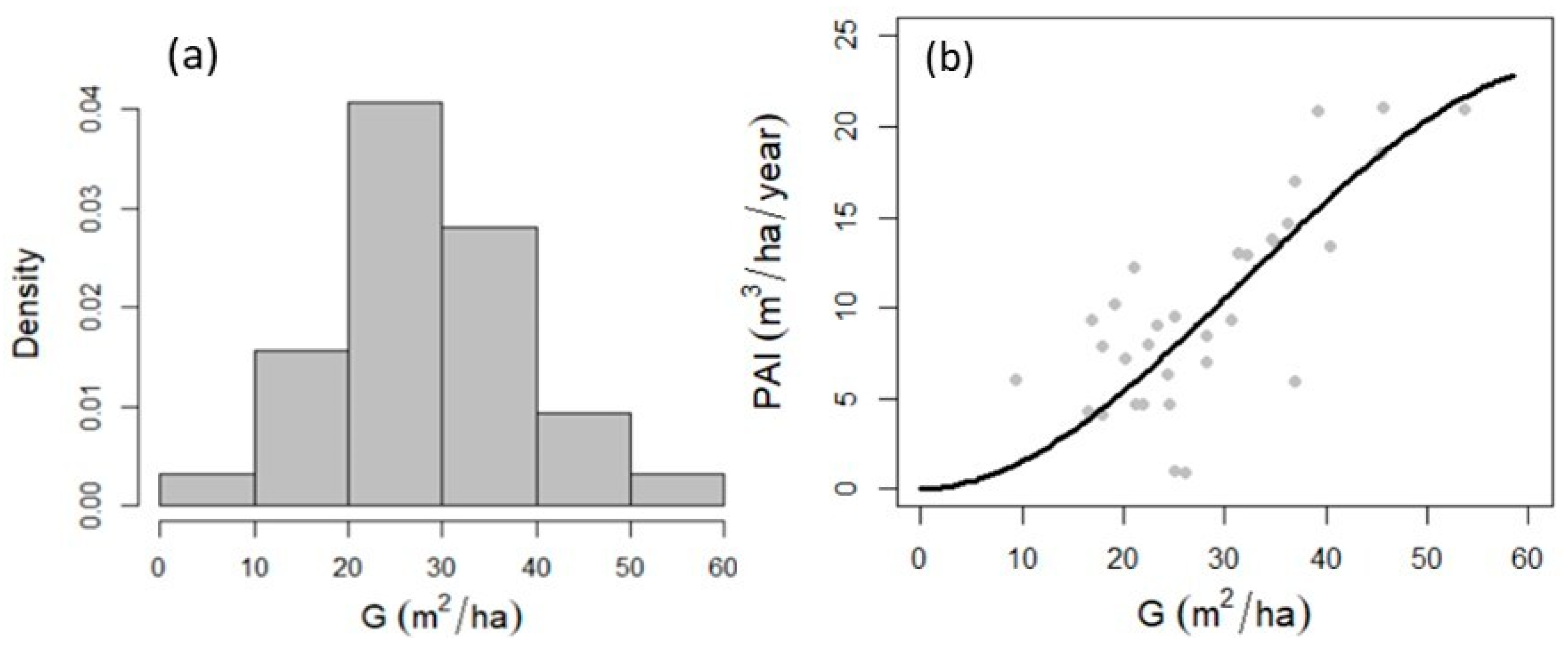
3.3. Relationship between Forest Density, Diversity and Production

The stepwise linear regression identified the principal variables that determine the productivity in the multispecies and uneven-aged forests of the Sierra Madre Occidental. The equation selected to predict PAI is given below:
PAI = a × N + b × SDI + c × Hmean + d × Hill .
where P A I is the periodic annual increment (m3/ha/year); N is the number of individuals per hectare; SDI is Reineke’s Stand-density Index; Hmean is mean height; Hill is Hill number; and a , b , c , and d are the parameter estimates.
Table 2 shows the parameter estimates, residual standard error (RSE), and coefficient of determination (R2) of Equation (3). All parameters are significant (p ≤ 0.05) and the residuals were uniformly distributed. Interestingly, the coefficient d is negative, i.e., production is reduced considerably with increasing tree species diversity.
According our PAI data, the residual density is a principal element affecting forest production. Figure 5 shows, as an example, the relation between basal area and production based on our data ( PAI =   0.000788 × G 1 3 0.0000130 × G 1 4 , R2 = 0.81). Any attempt to generalize or simplify this relation at high densities should be based on a careful analysis of additional variables, including species composition, structure, and climate.
According to the relation between basal area and production, there is overwhelming evidence that production is significantly affected by forest density (Figure 5). This study shows that considerable loss in production can be expected if forest densities are reduced below 20 m2/ha. On the other hand, there are considerable potential gains in production if density is allowed to increase. The distribution of forest densities in our field plots and the density-production relation for Group 1 are shown in Figure 6.
Assuming that the five-yearly basal area increment (∆G, m2/ha) may be estimated as a function of basal area (G) by the following equation (derived from this study, R2 = 0.90, Δ G = 0.005287 × G 2 0.00006816 × G 3 ) , it is possible to estimate the number of years required to raise an unproductive low density stand of 15 m2/ha to a more productive one of almost 25 m2/ha. The number of years required to reach and acceptable basal area of 25 m2/ha, assuming an unproductive initial basal area of 15 m2/ha, is shown in Table 3.
At least 35 years without income from timber sales are needed to raise the unproductive basal area of 15 m2/ha to a more productive level of 25 m2/ha. Such examples demonstrate the dramatic effects of low forest densities for the communities which depend on the forest for income, and that low-density forest properties may need long recovery periods to attain acceptable levels of basal area.

4. Discussion

4.1. Groups of Field Plots and Maximun Forest Density

The high natural forests in the Region Madrense in Durango State exhibited a range of complex structures and changing spatial patterns, and it was surprising that after more than 100 years of harvesting activities by the local communities, the tree species diversity showed still a high level of complexity. The results of this study did not reveal significant differences in tree diversity between well-defined field groups of plots that significantly differed in other site variables. However, the degree to which selective management may have caused changes in forest structure and species composition in the Region Madrense, which represents the most important ecotone of the SMO, has not been assessed in sufficient detail [17,24]. The preservation of species richness in these complex forest ecosystems requires new methods of management. Accordingly, Gadow et al. [3] presented new retention strategies for selectively managed natural forests. They found that methods that do not prescribe how much to harvest but specify the residual forest in terms of tree species and dimensions, the structure, density, and diversity remaining after the harvest, were especially relevant.
Several new permanent forest observational networks have been established since the turn of the 20th century. Individual scientists have identified a real need for permanent monitoring that was not provided by the NFI’s in their countries. An example of such an initiative is the Mexican permanent plot network, which provided essential information in this study. Another example is the Forest Observational Network of the Beijing Forestry University, which includes several very large field plots with mapped trees in the mixed deciduous forests of Northeastern China, in the northern pine-oak forests, and in the central and western Abies-Picea mountain forests of China [44]. Large permanent plots provide opportunities for evaluating effects of scale [28], while networks of regularly spaced small plots enable scientists to study environmental response gradients. Both types are useful for the evaluation of the effects of forest density and the degree of site occupancy on forest production.
In this study, three groups of plots, which described distinctly different forest structures at the SMO, were identified. These forest types showed significant differences in N, G, Dq, Ho, and PAI. This result may be an indication that differences in forest density are mainly the result of management. The differences might also be caused by forest gaps created by small-scale disturbances that occur in these forests, like windthrow, bark beetles, and forest fires. However, the site variables used in the Kruskal–Wallis Test probably had a high level of collinearity, and it is therefore necessary to use other statistical techniques like ordination methods (e.g., principal component analysis, Detrended Correspondence Analysis) to describe which of these structural variables are the underlying factors that cause plots dissimilarity. Several other studies found that site occupation is an important property in a multispecies natural forest, and density management is a key to the successful use of the unique forest resources of the Region Madrense [6,16,24]. On the other hand, dominant height has the advantage of being hardly influenced by stand management measures such as thinning [38], although it can be affected by very low or very high stand densities [45]. In addition, forest structural attributes, such as number of trees and average tree size, may affect biomass productivity in natural forests [46]. Production in multispecies natural forests normally depends on site conditions, structural attributes, species composition, and forest density, as well as the interaction between these factors [47,48,49].

4.2. Maximun Forest Density

The limiting density estimate for Durango in this study was ln ( N m a x ) = l n ( 118 , 434.6 ) 1.536   × ln ( D q ) . Hernández et al. [50] obtained similar results for the natural forests in Hidalgo, Mexico, where the values of α and β were 105,550.7 and 1.535, respectively. Results of the maximum density analysis indicate that the relationship between the mean squared diameter and tree density well describes the phase of stand development and is related to self-thinning and crown closure dynamics of these species-rich forests [51].

4.3. Relationship between Forest Density and Production

Ambiguity may be caused by different interpretations of forest production: (i) Net production, i.e., the periodic annual volume (or biomass) increment of all live trees plus ingrowth and the volume of trees removed in thinnings; (ii) gross production, i.e., net production plus the volume of trees lost to mortality; and (iii) accretion, i.e., the volume increment of only those trees that survived during the growth period [52]. The differentiation between definitions of forest production is important, as each may result in different density–production patterns [52]. Confusions arising from previous work in forest density–production relationships are caused by the fact that the same density may include considerable differences in forest structure and diversity. The same forest density may include few large trees or many small ones. The same density may be found on poor or good sites. Accordingly, to be realistic, estimates of forest production in multi-age forests need to consider such different patterns, as exemplified by this study.
Different models for the relation between forest density and production have been used. Based on previous work, Allen and Burkhart [53] defined three theoretical relationships between forest production and density, as "increasing," "optimal," and "constant." They pointed out that this relation is usually uncertain for very high densities. The PAI model developed in the present study included the site variables N, SDI, Hmean, and Hill number in their formulation. However, the most important contribution of the variance, explained by Equation (3), came from the stand density index, which provides a measure of density that is independent of age and site quality [54]. Significant evidence has been presented that forest density influences production in plantation monocultures [55,56] and natural forests [16,24]. These results confirm earlier findings obtained with fewer observations about the potential theoretical relationships between forest density and production [38,57]. Our results show that considerable loss in production can be expected if basal areas of forests are reduced below 20 m2/ha. Schütz et al. [58] found that a residual basal area of 20–24 m2/ha was appropriate for successful beech regeneration in a forest characterized by a mosaic of irregular groups.

5. Conclusions

In this study, three groups of forest stands, which described distinctly different forest structures at the SMO, were identified. These forest types showed significant differences in the number of trees per hectare, basal area per hectare, quadratic mean diameter, dominant height, and periodic annual increment. Tree species diversity was similar between the three groups of stands. This result may be an indication that differences in forest density are mainly the result of forest management. According our study, the site variables N, SDI, Hmean, and Hill number were the the principal elements affecting forest production of these forests. One of the surprising results, confirming earlier studies (e.g., [24]), is the fact that the potential production in some areas was high, and exceeded 20 m3/ha/year provided a residual density of at least 30 m2/ha was maintained.
Although the results indicate that the continuous cover forestry management system used in Durango’s community forests has not affected significantly tree diversity, studies in other regions of the world have shown that there is no unique and ideal diameter distribution in multispecies forests [59]. These forests may exhibit a great variety of structures with varying proportions of small-, medium-, and large-sized trees. Tree species compositions are often highly variable in natural forest communities. For this reason, it is necessary to develop new methods for ensuring sustainable production in natural forests based on forest density and particular species distribution.
Most of the local Mexican Ejidos and Comunidades in the study region have been able to withstand the pressure of commercial interests to convert the natural ecosystems to even-aged monocultures. An alternative method for controlling sustainable harvests in multispecies natural forests is an approach based on residual basal area. The general concept is based on the premise that a post-harvest residual density is defined and that the residual density is distributed over specific tree sizes and tree species [3]. Such a method would not only ensure that the productive potential can be sustained, but also that the main features of the natural system are maintained. Details of such a management system need to be worked out to meet the specific demands of the communal forests of the Sierra Madre Occidental.

Author Contributions

Conceptualization, J.R.P.-M. and K.v.G.; formal analysis J.R.P.-M. and K.v.G.; Methodology, J.R.P.-M. and K.v.G.; writing—original draft, J.R.P.-M., J.J.C.-R. and K.v.G.; writing—review and editing, J.B.-R., C.P. and P.M.L.-S. All authors have read and agreed to the published version of the manuscript.

Funding

Data collection for this research was funded by the National Forestry Commission.

Acknowledgments

This study was supported by the National Forestry Commission (CONAFOR) and the Mexican National Council for Science and Technology (CONACYT). We thank the two anonymous reviewers whose comments have greatly improved this manuscript.

Conflicts of Interest

The authors declare no conflict of interest. The funding sponsors had no role in the design of the study; in the collection, analyses, or interpretation of data; in the writing of the manuscript, or in the decision to publish the results.

References

  1. Von Gadow, K.; Hui, G. Modelling Forest Development; Kluwer Academic: Dordrecht, The Netherlands, 1999. [Google Scholar]
  2. Burkhart, H.E.; Tomé, M. Modelling Forest Trees and Stands; Springer: Dordrecht, The Netherlands, 2012. [Google Scholar]
  3. Von Gadow, K.; Zhao, X.H.; Corral-Rivas, J.J. Retention Strategies for Multi-Species Forests. In Proceedings of the International Symposium for the 50th Anniversary of the Forestry Sector Planning in Turkey, Antalya, Turkey, 26–28 November 2013. [Google Scholar]
  4. Von Gadow, K.; Kotze, H. Tree survival and maximum density of planted forests—Observations from South African spacing studies. For. Ecosyst. 2014, 1, 21. [Google Scholar]
  5. Pretzsch, H.; Schütze, G. Effect of tree species mixing on the size structure, density, and yield of forest stands. Eur. J. For. Res. 2016, 135, 1–22. [Google Scholar] [CrossRef]
  6. Quiñonez-Barraza, G.; Tamarit-Urias, J.C.; Martínez-Salvador, M.; García-Cuevas, X.; de los Santos-Posadas, H.M.; Santiago-García, W. Maximum density and density management diagram for mixed-species forest in Durango, Mexico. Rev. Chapingo Ser. Cie. For. Ambiente 2017, 24, 73–90. [Google Scholar] [CrossRef]
  7. West, P.W. Comparison of stand density measures in even-aged regrowth eucalypt forest of southern Tasmania. Can. J. For. Res. 1983, 13, 22–31. [Google Scholar] [CrossRef]
  8. Harper, J.L. Population Biology of Plants; Academic Press: London, UK, 1977. [Google Scholar]
  9. Diamantopoulou, M.J.; Özçelik, R.; Crecente-Campo, F.; Eler, Ü. Estimation of Weibull function parameters for modelling tree diameter distribution using least squares and artificial neural networks methods. Biosyst. Eng. 2015, 133, 33–45. [Google Scholar] [CrossRef]
  10. Arias-Rodil, M.; Diéguez-Aranda, U.; Álvarez-González, J.G.; Pérez-Cruzado, C.; Castedo-Dorado, F.; González-Ferreiro, E. Modeling diameter distributions in radiata pine plantations in Spain with existing countrywide LiDAR data. Ann. For. Sci. 2018, 75, 36. [Google Scholar] [CrossRef] [Green Version]
  11. Gadow, K.V. Untersuchungen Zur Konstruktion Von Wuchsmodellen Für Schnellwüchsige Plantagenbaumarten; Universität München: München, Germany, 1987. [Google Scholar]
  12. Rubin, B.D.; Manion, P.D.; Faber-Langendoen, D. Diameter distributions and structural sustainability in forests. For. Ecol. Manag. 2006, 222, 427–438. [Google Scholar] [CrossRef]
  13. Calzado, C.A.; Torres, A.E. Modelling diameter distributions of Quercus suber L. stands, in “Los Alcornocales” natural park (Cádiz-Málaga, Spain) by using the two parameter Weibull functions. For. Syst. 2013, 22, 15–24. [Google Scholar] [CrossRef] [Green Version]
  14. Pretzsch, H.; Biber, P. Tree species mixing can increase stand density. Can. J. For. Res. 2016, 46, 1179–1193. [Google Scholar] [CrossRef] [Green Version]
  15. Torres-Rojo, J.M. Exploring volume growth-density of mixed multiaged stands in northern Mexico. Agrociencia 2014, 48, 447–461. [Google Scholar]
  16. Corral-Rivas, J.J.; Torres-Rojo, J.M.; Lujan-Soto, J.E.; Nava-Miranda, M.G.; Aguirre-Calderón, O.A.; Gadow, K.V. Density and production in the natural forest of Durango/Mexico. Allg. Fort. Jagdztg. 2016, 187, 93–103. [Google Scholar]
  17. González-Elizondo, M.S.; González-Elizondo, M.; Tena-Flores, J.A.; Ruacho-González, L.; López-Enríquez, I.L. Vegetación de la Sierra Madre Occidental, México: Una síntesis. Acta Bot. Mex. 2012, 100, 351–403. [Google Scholar] [CrossRef] [Green Version]
  18. González-Elizondo, M.S.; González-Elizondo, M.; Ruacho-González, L.; López-Enríquez, I.L.; Tena-Flores, J.A. Ecosystems and diversity of the Sierra Madre Occidental. In Proceedings of the Merging Science and Management in a Rapidly Changing World: Biodiversity and Management of the Madrean Archipelago III and 7th Conference on Research and Resource Management in the Southwestern Deserts, Tucson, AZ, USA, 1–5 May 2012; Gottfried, G.J., Ffolliott, P.F., Gebow, B.S., Eskew, L.G., Collins, L.C., Eds.; RMRS-P. Department of Agriculture, Forest Service: Fort Collins, CO, USA, 2013; Volume 67, pp. 204–211. [Google Scholar]
  19. Corral-Rivas, J.J.; Reyes, R.I.; Wehenkel, C.; Aguirre-Calderón, O.A.; Gadow, K. A network of forest observational studies in Durango (Mexico). In Proceedings of the International Workshop at Beijing Forestry University, Beijing, China, 20–21 September 2012; Zhao, X.H., Zhang, C.Y., Gadow, K., Eds.; Beijing Forestry University: Beijing, China, 2012; pp. 125–138. [Google Scholar]
  20. Weibull, W. A statistical distribution function of wide applicability. J. Appl. Mech. 1951, 18, 293–297. [Google Scholar]
  21. Venables, W.N.; Ripley, B.D. Modern Applied Statistics with S, 4th ed.; Springer: New York, NY, USA, 2002. [Google Scholar]
  22. Team, R.C. R: A Language and Environment for Statistical Computing; R Foundation for Statistical Computing: Vienna, Austria, 2019; Available online: https://www.R-project.org/ (accessed on 21 December 2019).
  23. Martínez-Fernández, J.; Chuvieco, S.E. Tipologías de incidencia y causalidad de incendios forestales basadas en análisis multivariante. Ecología 2003, 17, 47–63. [Google Scholar]
  24. Corral-Rivas, J.J.; González-Elizondo, M.S.; Lujan-Soto, J.E.; Gadow, K.V. Effects of density and structure on production in the communal forests of the Mexican Sierra Madre Occidental. South. For. 2019, 81. [Google Scholar] [CrossRef]
  25. Reineke, L.H. Perfecting a stand-density index for even-aged forests. J. Agric. Res. 1933, 46, 627–638. [Google Scholar]
  26. Oliver, C.D.; Larson, B.C. Forest Stand Dynamics. Update Edition; Yale School of Forestry & Environmental Studies Other Publications: New York, NY, USA, 1996; Available online: https://elischolar.library.yale.edu/fes_pubs/1 (accessed on 21 December 2019).
  27. Zeide, B. Optimal stand density: A solution. Can. J. For. Res. 2004, 34, 846–854. [Google Scholar] [CrossRef]
  28. Zhang, C.Y.; Zhao, X.H.; Gadow, K.V. Maximum density patterns in two natural forests: An analysis based on large observational field studies in China. For. Ecol. Manag. 2015, 346, 98–105. [Google Scholar] [CrossRef]
  29. Koenker, R. Quantreg: Quantile Regression. R Package Version 5.4. 2019. Available online: https://CRAN.R-project.org/package=quantreg (accessed on 21 December 2019).
  30. Edwards, B.L.; Allen, S.T.; Braud, D.H.; Keim, R.F. Stand density and carbon storage in cypress-tupelo wetland forests of the Mississippi River Delta. For. Ecol. Manag. 2019, 441, 106–114. [Google Scholar] [CrossRef]
  31. Jost, L. Entropy and diversity. Oikos 2006, 113, 363–374. [Google Scholar] [CrossRef]
  32. Aerts, R.; Honnay, O. Forest restoration, biodiversity and ecosystem functioning. BMC Ecol. 2011, 11, 29. [Google Scholar] [CrossRef] [PubMed] [Green Version]
  33. Chao, A.; Chun-Huo, C.; Lou, J. Unifying Species Diversity, Phylogenetic Diversity, Functional Diversity, and Related Similarity and Differentiation Measures Through Hill Numbers. Annu. Rev. Ecol. Evol. Syst. 2014, 45, 297–324. [Google Scholar] [CrossRef] [Green Version]
  34. Hill, M. Diversity and evenness: A unifying notation and its consequences. Ecology 1973, 54, 427–431. [Google Scholar] [CrossRef] [Green Version]
  35. Elliott, M. Marine science and management means tackling exogenic unmanaged pressures and endogenic managed pressures—A numbered guide. Mar. Pollt. Bull. 2011, 62, 651–655. [Google Scholar] [CrossRef]
  36. Leinster, T.; Cobbold, C.A. Measuring diversity: The importance of species similarity. Ecology 2012, 93, 477–489. [Google Scholar] [CrossRef] [Green Version]
  37. Gadow, K.V.; Zhang, C.Y.; Wehenkel, C.; Pommerening, A.; Corral-Rivas, J.J.; Korol, M.; Myklush, S.; Hui, G.Y.; Kiviste, A.; Zhao, X.H. Forest Structure and Diversity. In Continuous Cover Forestry, 2nd ed.; Pukkala, T., Gadow, K.V., Eds.; Springer: Dordrecht, The Netherlands, 2011; pp. 29–84. [Google Scholar]
  38. Assmann, E. Principles of Forest Yield Study; Pergamon Press: New York, NY, USA, 1970. [Google Scholar]
  39. Pretzsch, H.; del Río, M.; Ammer, C.; Avdagic, A.; Barbeito, I.; Bielak, K.; Brazaitis, G.; Coll, L.; Dirnberger, G.; Drössler, L.; et al. Growth and yield of mixed versus pure stands of Scots pine (Pinus Sylvestris L.) and European beech (Fagus sylvatica L.) analysed along a productivity gradient through Europe. Eur. J. For. Res. 2015, 134, 927–947. [Google Scholar] [CrossRef] [Green Version]
  40. Vanclay, J.K. Modelling Forest Growth and Yield; Applications to Mixed Tropical Forest; CAB International: Wallingford, UK, 1994. [Google Scholar]
  41. Marziliano, P.A.; Menguzzato, G.; Scuderi, A.; Corona, P. Simplified methods to inventory the current annual increment of forest standing volume. Iforest 2012, 5, 276–282. [Google Scholar] [CrossRef] [Green Version]
  42. Huang, S.F.; Cheng, C.H. GMADM-based attributes selection method in developing prediction model. Qual. Quant. 2012, 47, 3335–3347. [Google Scholar] [CrossRef]
  43. Shapiro, S.S.; Wilk, M.B. An analysis of variance Test for normality (complete samples). Biometrika 1965, 52, 591–611. [Google Scholar] [CrossRef]
  44. Zhao, X.H.; Corral-Rivas, J.J.; Zhang, C.Y.; Temesgen, H.; Gadow, K.V. Forest observational studies-an essential infrastructure for sustainable use of natural resources. For. Ecosyst. 2014, 1, 8. [Google Scholar] [CrossRef] [Green Version]
  45. Vallet, P.; Perot, T. Tree diversity effect on dominant height in temperate forest. For. Ecol. Manag. 2016, 381, 106–114. [Google Scholar] [CrossRef]
  46. Ouyang, S.; Xiang, W.; Wang, X.; Xiao, W.; Chen, L.; Li, S.; Sun, H.; Deng, X.; Forrester, D.I.; Zeng, L.; et al. Effects of stand age, richness and density on productivity in subtropical forests in China. J. Ecol. 2019, 107, 2266–2277. [Google Scholar] [CrossRef]
  47. Kelty, M.J. Comparative productivity of monocultures and mixed species stands. In The Ecology and Silviculture of Mixed-Species Forests; Kelty, M.J., Larson, B.C., Oliver, C.D., Eds.; Kluwer Academic Publishers: Dordrecht, The Netherlands, 1992. [Google Scholar]
  48. Garber, S.M.; Maguire, D.A. Stand productivity and development in two mixed-species spacing trials in the Central Oregon Cascades. For. Sci. 2004, 50, 92–105. [Google Scholar]
  49. Jacob, M.; Leuschner, C.; Thomas, F.M. Productivity of temperate broad-leaved forest stands differing in tree species diversity. Ann. For. Sci. 2010, 67, 503. [Google Scholar] [CrossRef] [Green Version]
  50. Hernández, R.J.; García, M.; Muíoz, F.; García-Cuevas, J.; Sáenz, R.T.; Flores, L.C.; Hernández, R.A. Density management guide for natural Pinus teocote Schecht Cham Forest in Hidalgo. Rev. Mex. Cienc. For. 2013, 4, 62–76. [Google Scholar]
  51. VanderSchaaf, C.L.; Burkhart, H.E. Using segmented regression to estimate stages and phases of stand development. For. Sci. 2008, 54, 167–175. [Google Scholar]
  52. Nyland, R.D. Silviculture Concepts una Applications; Waveland Press: Long Grove, IL, USA, 2016; p. 680. [Google Scholar]
  53. Allen, M.G.; Burkhart, H.E. Growth-density relationships in Loblolly Pine plantations. For. Sci. 2018, 65, 250–264. [Google Scholar] [CrossRef]
  54. Harrington, T.B. Silvicultural Approaches for Thinning Southern Pines: Method, Intensity, and Timing. Available online: http://www.gfc.state.ga.us/resources/publications/SilviculturalApproaches.pdf (accessed on 21 December 2019).
  55. Tewari, V.P.; Gadow, K.V. Modelling potential density limiting survival, stand density and basal area growth for pure even-aged Dalbergia sissoo stands in a hot arid region of India. For. Trees Livelihoods 2008, 18, 133–150. [Google Scholar] [CrossRef]
  56. Dickel, M.; Kotze, H.; Gadow, K.V.; Zucchini, W. Growth and Survival of Eucalyptus grandis—A Study based on Modelling Lifetime Distributions. MCFNS 2010, 2, 20–30. [Google Scholar]
  57. Thomasius, H.O.; Thomasius, H. Ableitung eines Verfahrens zur Berechnung der ertragskundlich optimalen Bestandesdichte. Beiträge F. D. Forstwirtsch. 1978, 12, 79. [Google Scholar]
  58. Schütz, J.P.; Saniga, M.; Diaci, J.; Vrška, T. Comparing close-to-nature silviculture with processes in prime forests: Lessons from Central Europe. Ann. For. Sci. 2016, 73, 911–921. [Google Scholar] [CrossRef] [Green Version]
  59. Torres-Rojo, J.M. Sostenibilidad del volumen de cosecha calculado con el método mexicano de montes. Madera Bosques 2000, 6, 57–72. [Google Scholar] [CrossRef] [Green Version]
Figure 1. Spatial distributions of field plots by group in the state of Durango. The plots were divided into three groups, which differed in terms of basal area, diameter distribution, and the relationship between number of trees and average tree size. Plot affiliation to a particular group is indicated by one of three groups.
Forests 11 00307 g001
Figure 2. Four characteristics of the three groups of plots. (a) The relationship between number of trees (N) and basal area (G); (b) the relationship between number of trees (N) and dominant height (Ho); (c) the diameter distributions; and (d) the height distributions.
Forests 11 00307 g002
Figure 3. Forest conditions by class of density. Width represents relative density within each bin and the boxplot represents the quartiles. All the variables showed significant differences (p ≤ 0.05) according to Dunn’s test, except for the number of species, which was not significantly different among groups. N, G, Dq, Ho, and PAI are defined in Table 1.
Forests 11 00307 g003
Figure 4. Maximum density estimated by percentile regression for the 217 plots. The three forest types are identified by different colors. Dq: Quadratic mean diameter.
Forests 11 00307 g004
Figure 5. Assumed relation between basal area and production based on our data.
Forests 11 00307 g005
Figure 6. Distribution of forest densities in our field plots and the density-production relation for Group 1. (a) Distribution of basal area; (b) relation between basal area and production.
Forests 11 00307 g006
Table 1. Summary statistics of the 217 plots used in this study.
PlotFirst InventorySecond Inventory
VariableMeanMaxMinSdMeanMaxMinSd
N623.782264.00120.00281.30624.182152.00144.00275.91
G (m2/ha)21.1653.633.158.2023.3158.523.928.98
Dq (cm)21.3234.1012.404.2822.3436.0013.404.44
V (m3/ha)188.55604.2112.04106.19221.04709.2016.57124.28
Ho (m)16.8229.505.204.8018.1831.605.805.19
S7.9115.001.002.418.1716.001.002.48
W (ton/ha)104.88306.676.3062.53123.92374.758.9073.15
PAI (m3/ha/year) 6.5021.660.244.40
N: Number of trees per hectare; G: Basal area; Dq: Quadratic mean diameter; V: Volume; Ho: Dominant height, the mean height of the 100 thickest trees per hectare; S: Number of tree species in plot; W: Dry biomass; PAI: Periodic annual increment; Sd: Standard deviation.
Table 2. Coefficients of Equation (3) for estimating the relation between periodic production (PAI).
ParameterEstimateStandard ErrorT Valuep-ValueRSER2
a−0.0044650.001119−3.9919.06 × 10−50.120.85
b0.0183270.0021628.4773.85 × 10−15
c0.2261100.0536004.2183.64 × 10−5
d−0.3749810.074914−5.0051.17 × 10−6
RSE is the residual standard error and R2 is the coefficient of determination.
Table 3. Basal area annual increment for forest with low density.
G (m2/ha)∆G (m2/ha/year)Time Required (years)
15.000.00000
15.960.95955
17.031.069610
18.231.196615
19.571.343620
21.081.513925
22.791.711330
24.731.939835

