Article

Multi-Sensor Prediction of Stand Volume by a Hybrid Model of Support Vector Machine for Regression Kriging

1
Key Laboratory of Wetland Ecology and Environment, Northeast Institute of Geography and Agroecology, Chinese Academy of Sciences, Changchun 130102, China
2
University of Chinese Academy of Sciences, Beijing 100049, China
3
National Earth System Science Data Center, Beijing 100101, China
*
Author to whom correspondence should be addressed.
Forests 2020, 11(3), 296; https://doi.org/10.3390/f11030296
Submission received: 23 January 2020 / Revised: 25 February 2020 / Accepted: 5 March 2020 / Published: 6 March 2020

Abstract

:
Quantifying stand volume through open-access satellite remote sensing data supports proper management of forest stand. Because of limitations on single sensor and support vector machine for regression (SVR) as well as benefits from hybrid models, this study innovatively builds a hybrid model as support vector machine for regression kriging (SVRK) to map stand volume of the Changbai Mountains mixed forests covering 171,450 ha area based on a small training dataset (n = 928). This SVRK model integrated SVR and its residuals interpolated by ordinary kriging. To determine the importance of multi-sensor predictors from ALOS and Sentinel series, the increase in root mean square error (RMSE) of SVR was calculated by removing the variable after the standardization. The SVRK model achieved accuracy with mean error, RMSE and correlation coefficient in –2.67%, 25.30% and 0.76, respectively, based on an independent dataset (n = 464). The SVRK improved the accuracy of 9% than SVR based on RMSE values. Topographic indices from L band InSAR, backscatters of L band SAR, and texture features of VV channel from C band SAR, as well as vegetation indices of the optical sensor were contributive to explain spatial variations of stand volume. This study concluded that SVRK was a promising approach for mapping stand volume in the heterogeneous temperate forests with limited samples.

1. Introduction

Forest stand volume, as an ecosystem service, forms the basis for decision-making at diverse levels [1]. Spatial explicit information on forest stand volume is critical for indirect estimation of aboveground biomass for quantifying carbon sequestration and carbon dioxide exchange [2]. Field-based inventories of forest stand volume, the conventional approach, is costly and spatially limited [3]. Progress has been made in mapping forest volume by remote sensing modeling based on multisource satellite and inventory data for spatially continuous and temporally uniform predictions [4,5]. Those remote sensing algorithms were divided into two categories, i.e., physical and empirical models, and the latter included statistical regressions, machine learning techniques, and hybrid approaches [6,7,8]. Physically based models depend on numerous geometry and biochemistry factors, which may not be readily available [9,10]. Statistical regressions model stand volume by estimating equation parameters related to remote sensing variables [11,12]. These regressions have advantages on modeling explicit relationships and applications at large scales [13,14]. Machine learning algorithms have no assumption on input variable distribution, type and number, which achieve robust and accurate predictions on complex relationships [15,16]. Among the various machine learning techniques, support vector machine is acclaimed for its capacity of dealing with small training datasets in remote sensing-based classification [17,18]. After the re-design to predict quantitative outputs and solve regression problems, this algorithm came to be the support vector machine for regression (SVR) and acquired wide successes in stand volume modeling [19,20]. Hybrid approaches involve either the statistical regression or machine learning model between the target variable and remote sensing predictors, interpolating residuals of predictions by kriging, and combining them [21,22,23]. Those two-step approaches both consider the spatial heterogeneity conveyed by remote sensing predictors and autocorrelation of neighboring observed data [24,25]. Those approaches, especially machine learning combined ordinary kriging of residuals such as artificial neural network kriging (ANNK) and random forest kriging (RFK), have yielded accurately spatial predictions [26,27]. However, support vector machine for regression kriging (SVRK) modeling for mapping forest volume has rarely been tested and reported.
Stand volume modeling with open-access satellite data has been comparable, repeatable, and has long-term monitoring [28,29,30]. With the global coverage, Sentinel-1 C band synthetic aperture radar (SAR) and Sentinel-2 multispectral instrument (MSI) images provide capabilities for stand volume modeling using both active and passive remote sensing techniques [31,32]. The Advanced Land Observing Satellite (ALOS/ALOS-2) Phased Array type L band SAR (PALSAR/PALSAR-2) from L band SAR have penetrability, which contain comprehensive information on the orientation and structure of tree canopy and stems within the pixel [33,34]. It makes the ALOS/ALOS-2 images with global observations particularly useful for stand volume mapping [35,36]. The ALOS digital surface model (DSM) from L band interferometric SAR (InSAR) with accurate values of elevation and can provide useful topographic indices to estimate stand volume [37,38,39]. Reported studies have explored the potential of multi-sensor data using the SVR in volume mapping [31,40,41]. However, how volume predictions would be affected by using SAR and MSI predictors based on the SVR deserves further exploration.
The Changbai Mountains Mixed forests, as the richest eco-region in temperate forests of northeastern China, play a key role in carbon cycles and ecosystem services both at regional and global scales [42,43,44,45]. Hence, in this study, we innovatively developed a SVRK model based on limited samples and open-access satellite predictors, and adopted it to map stand volume of the Changbai Mountains Mixed forests, a vital eco-region of temperate ecosystems. The specific objectives were to: (1) determine and compare the relationships of forest volume with multi-sensor variables from ALOS-2, Sentinel-1, Sentinel-2 and ALOS DSM; (2) map stand volume by the SVRK modeling; and (3) analysis spatial variations of stand volume and provide managerial suggestions for forest farms in the study area.

2. Materials and Methods

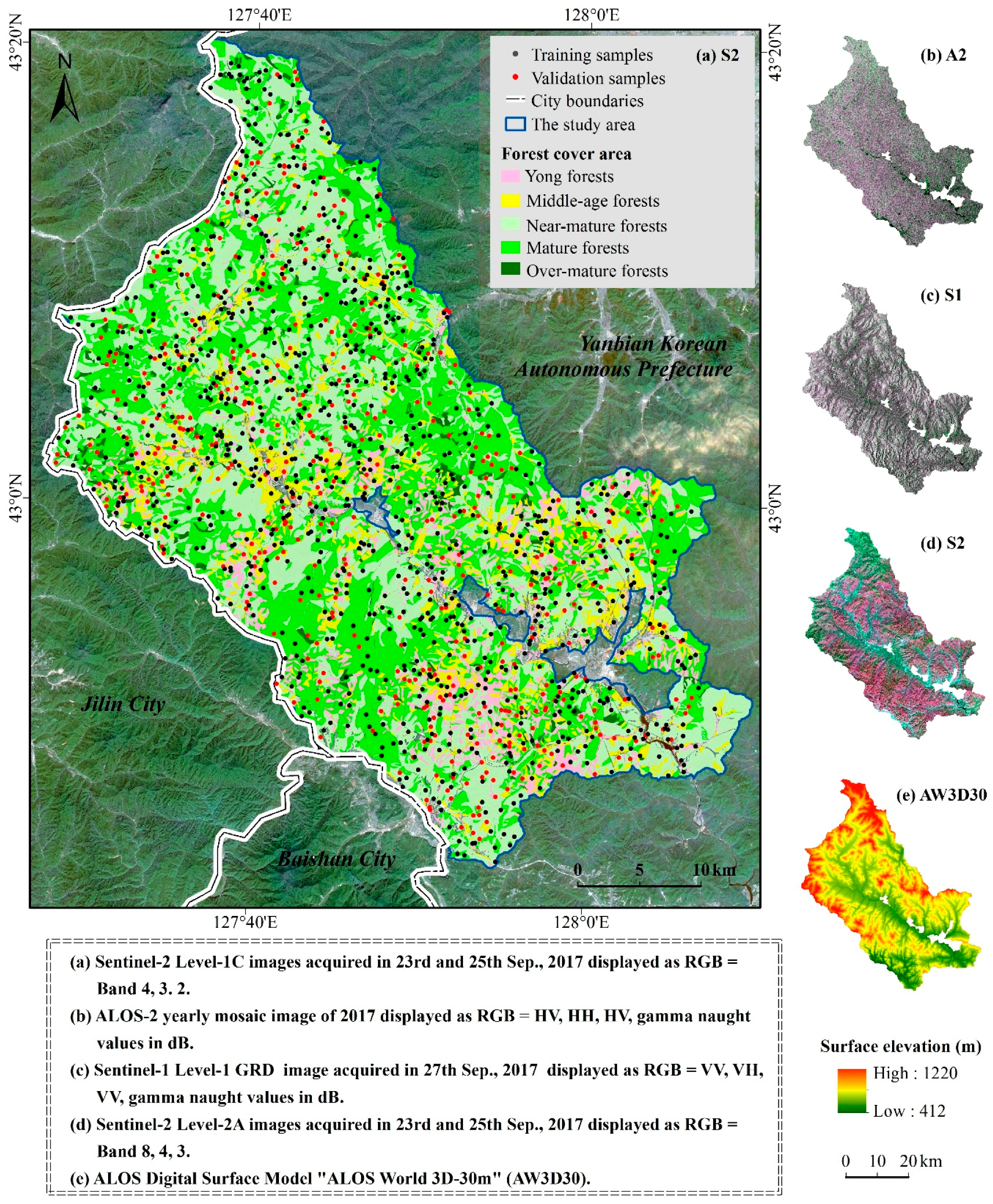
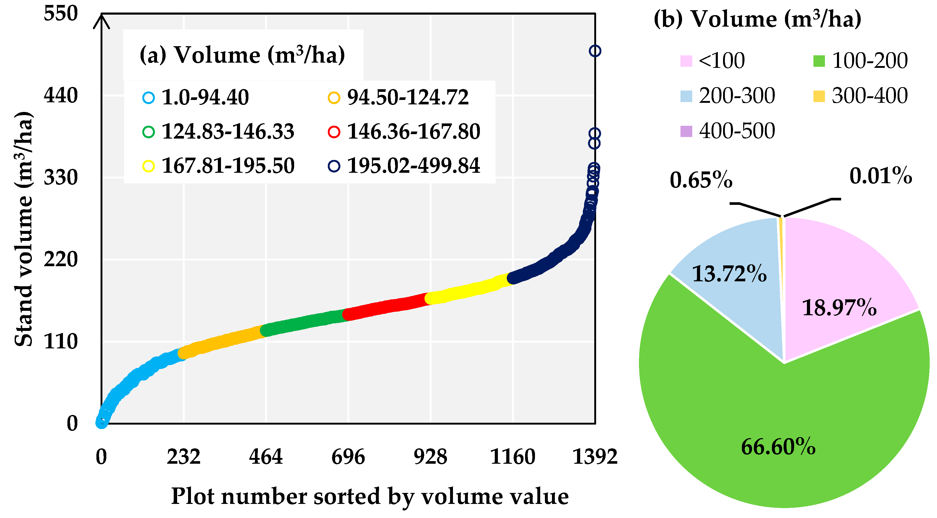
2.1. Study Area and Field-Measured Stand Volume

The study area covers 171,450 ha and 12 forest farms belonging to Forestry Bureau of Dunhua County (Figure 1). The site is located within the western mountainous area of Yanbian Korean Autonomous Prefecture of Jilin Province, northeast China. The climate is four-season, monsoon-influenced and humid continental, with an annual average temperature and precipitation of 3.28 °C and 632 mm, respectively [25]. Characterized by the dense cover of the Changbai Mountains mixed forests, the major forest types include deciduous broadleaved forest and mixed broadleaf-conifer forest with natural vegetation [43]. Dominant tree species include Tilia amurensis (Rupr.), Juglans mandshurica (Maxim.), Fraxinus mandschurica (Rupr.), Mongolian oak (Quercus spp.) and Betula platyphylla (Suk.). Typical soils are dark-brown earths, meadow, bog, chernozem, and peat soil.
The field campaign was carried out in September 2017. Stratified sampling design was used by masking non-forest areas and randomly generating the distribution of sampling plots in forest areas, while the plots that were impossible to access were replaced by the nearest sites. Following the national guidelines for forest resource survey [46], eight teams took part in collecting measured data under the same protocol. A total of 1392 squared 30 m by 30 m samples were established (Figure 1a). At each sample site, tree species, diameter at breast height (DBH, the diameter at 1.3 m from the ground), and tree height were measured and recorded. Age classes from young to over-mature were acquired from the forest manager’s archives at the local forestry bureau for further analysis (Figure 1a). Stand volume was estimated by DBH and tree height according to the National Standard of China: Tree volume tables (LY/T 1353–1999) [47]. The field-measured stand volume was from 1 to 499.8 m3/ha, and was divided into six levels with the same frequency, with the median and standard deviation (SD) value of 146.3 and 56.2 m3/ha, respectively (Figure 2a). The values of measured volume were mainly below 200 m3/ha with 85.57 % (Figure 2b). The 1,392 sampling sites were randomly divided into training (n = 928) and validation (n = 464) sets (Figure 1a) for training and assessing the models.

2.2. Satellite Data Pre-Processing and Derived Variables

The adopted multi-sensor satellite data are listed in Table 1. The 25-m ALOS-2 L band SAR yearly mosaic images of 2017 were downloaded from the ALOS Research and Application Project of EORC, the Japan Aerospace Exploration Agency to acquire the normalized backscatter coefficients (gamma naught values) (Table 2), which was sensitive to stand volume [36,48,49]. Images were converted to gamma naught values in decibel unit (dB) from 16-bit digital number (DN) (Figure 1b) using the following Equation (1) [50]:
γ 0 = 10 log 10 ( D N 2 ) 83
where γ 0 is gamma naught backscatter coefficient of horizontal transmit-horizontal channel (HH) or horizontal transmit-vertical channel (HV); DN is the polarization data in HH or HV.
Sentinel series images were downloaded from the Copernicus Sentinel Scientific Data Hub. The data included one Sentinel-1 C-band SAR and three Sentinel-2 MSI images. The SAR image was at a high-resolution (HR) Level-1 ground range detected (GRD) processing level with a pixel size of 10 m [51]. Promising results demonstrated that the normalized backscatter coefficients and texture features from Sentinel-1 images could improve forest parameter estimation [32,52]. Sentinel-1 Toolbox in SNAP software (version 6.0, European Space Agency, Paris, France) was used to acquire Sentinel-1 variables with a map projection (Figure 1c) by image calibration, speckle reduction using the Refined Lee Filter, terrain correction by the Range-Doppler, and grey level co-occurrence matrix analysis with 3 × 3-pixel window [52,53,54]. The Sentinel-2 Level 1C data were top-of-atmosphere reflectance, which were processed by orthorectification and registration [55]. The MSI data had 13 spectral bands, including four in 10 m (bands 2–4, 8), six in 20 m (band 5–7, 8a, 11–12), and three in 60 m (band 1, 9–10) spatial resolutions, respectively [55]. The 10-m Sentinel-2 Level 2A data (Figure 1d) were atmospherically corrected from the Level 1C data by the radiative transfer model-based SEN2COR atmospheric correction processor (version 2.5.5, European Space Agency, Paris, France), and were resampled by Sentinel-2 Toolbox in SNAP. Spectral indices were strongly related to reflectance, and were useful in volume mapping, especially some with red edge bands (band 5, 6, 7, and 8A) [56,57]. Totally, 26 variables from Sentinel-2 were selected and extracted based on previous findings (Table 2) [58,59].
The ALOS Global Digital Surface Model (AW3D30) used in this study was a global dataset generated from L band SAR images collected using the ALOS from 2006 to 2011 (Figure 1e). The data were download from the Japan Aerospace Exploration Agency to extract topographic indices from previous researches by Spatial Analyst of ArcGIS software (version 10.0, ESRI, RedLands, CA, USA) [60,61]. All remote sensing variables were re-projected into UTM Zone 52 WGS84, and then resampled to the 30 m pixel size by ArcGIS.

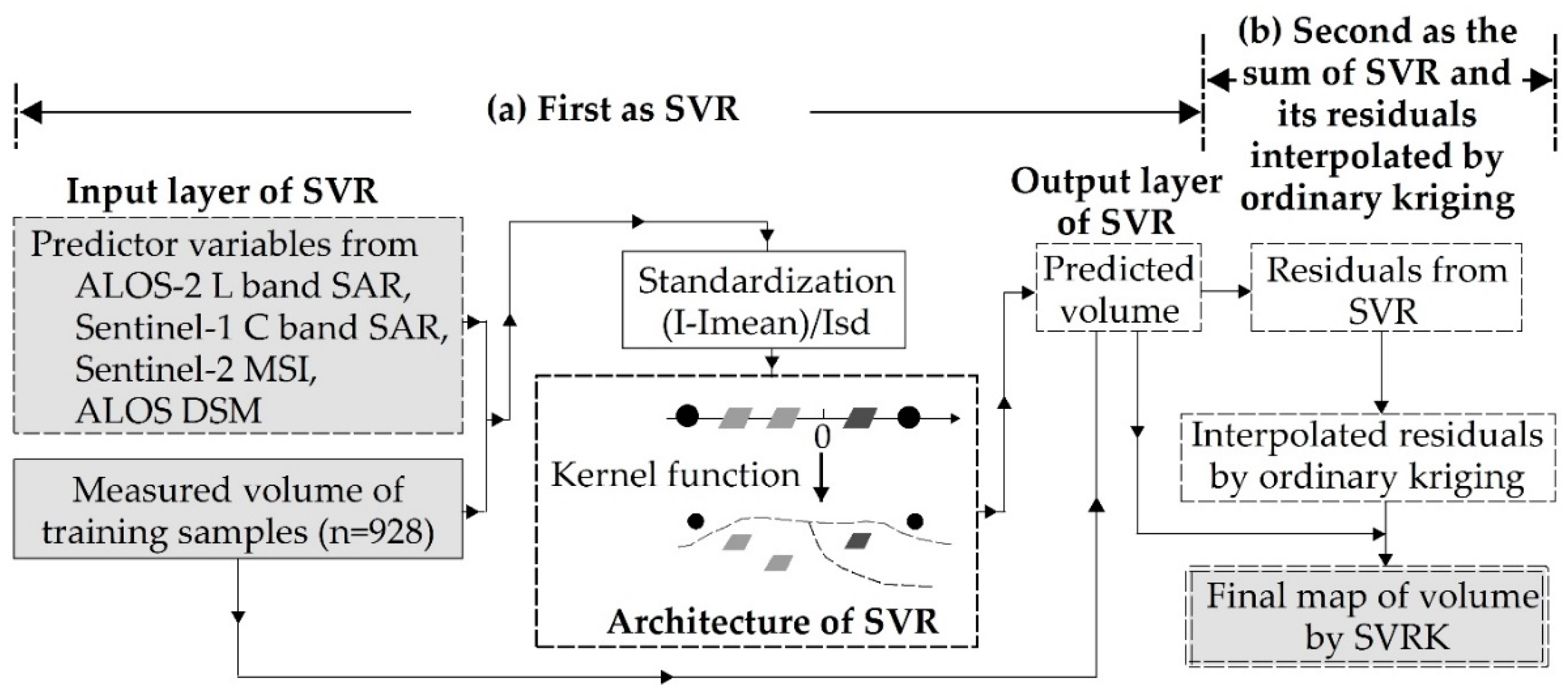
2.3. Support Vector Machine for Regression Kriging (SVRK) and Modeling Evaluation

The pairwise Pearson’s product-moment correlation analysis was operated to determine predictor variables from multi-sensor indices. It consisted of two steps: the selection of variables which were significantly related to field-measured volume (p < 0.05) as candidates; the disposal of candidates that were collinear (r ≥ 0.8), except the one that had the largest correlation coefficient with volume [62]. Those analyses were performed in SPSS software (version 21.0, IBM, Armonk, NY, USA).
The SVRK model built in this study is the extension of SVR, which integrated SVR prediction and estimation of the residuals by ordinary kriging using Equation (2). SVRK considers spatial parametric non-stationarity with the effects of multi-sensor predictors derived from the benefits of SVR. It also added the spatial dependence of the residuals interpolated through ordinary kriging to the estimated trend, as part of the spatial autocorrelation:
  V S V R K = V S V R + R O K .  
where: V S V R K , V S V R are predication of stand volume based on SVRK and SVR, respectively; R O K is the estimated residuals of volume from the SVR prediction.
The implementation of SVRK includes two steps, as shown in Figure 3. SVR is firstly used to model the relationship between stand volume and multi-sensor predictors, as a non-linear machine learning method. It uses kernel functions to project the training data onto a new hyperspace where complex non-linear patterns can be simply illustrated (Figure 3a) [63,64]. The optimal hyperspace, constructed by SVR, fits training data and predicts with minimal empirical risk [65]. The SMO (sequential minimal optimization) algorithm is used to solve the quadratic programming optimization problem step-by-step. It updates the SVR function, as shown in Equation 3, to reflect the new values until the Lagrange multipliers converged [66]:
f ( x ) = k = 1 n ( α k α k * ) K ( x k ,   x j ) + b
where x is a vector of the input predictors,   f ( x )   . is an optimal function developed by SVR, b is a constant threshold, K(xk, xj) is the radial basis function (RBF) kernel with the best bandwidth parameter σ, and α k are α k * the weights (Lagrange multipliers) with the constraints given in Equation 4.
{ k = 1 n ( α k + α k * ) = 0 0   α k ,   α k * C    
where C is the regularization parameter for balancing between the training error and model complexity.
In this study, SVR was conducted in WEKA software (version 3.8, The University of Waikato, Hamilton, New Zealand). Parameters of SVR, C, and σ, were selected by the smallest root mean square error (RMSE) based on field-measured volume in training dataset (Figure 1a). In order to determine the importance of multi-sensor predictors on volume mapping, the training data was standardized (Figure 3a), and then the increases in RMSEs were calculated as the predictors were excluded one by one from the SVR model.
At the second step, the residuals resulting from SVR are estimated using the ordinary kriging approach ( R O K ) (Figure 3b). Ordinary kriging, a widely used geostatistical technique, generates an optimal unbiased estimation by the semivariogram [67]. The semivariogram can be modeled by spherical, exponential, and Gaussian functions with three parameters—nugget, range and sill [68]. The nugget is an observation error, and sill is the magnitude of spatial autocorrelation [69]. Thus, the stronger spatial autocorrelation is denoted by the larger value of sill relative to nugget [69]. The range parameter shows on which distance the spatial autocorrelation does not influence any more [69]. The Kolmogorov-Smirnov test (K-S) was used to examine the distribution of residuals based on the stationarity assumption of ordinary kriging. The interpolation of residuals by ordinary kriging was conducted in ArcGIS with the smallest RMSE. Finally, volume prediction by SVRK ( V S V R K ) were acquired as the sum of V S V R and R O K .
The validation set (Figure 1a) was used to test the performance of volume mapping by SVRK based on the mean error (ME), RMSE, and correlation coefficient between the measured and predicted parameters (r) [70]. In order to better estimate accuracy, the mean measured value of stand volume (146.1 m3/ha in Figure 2a) was applied to divide the ME and RMSE. The relative improvement (RI) based on RMSE of SVRK over SVR was used as another index for accuracy evaluation [25].

3. Results

3.1. Relationship between Field-Measured Volume and Remote Sensing Variables

In total, 31 variables were significantly related to stand volume (p < 0.05) (Table 3), including seven from SAR, 20 from MSI, and four from DSM. The backscatters from different wavelengths all had strongly positive correlations with volume, while variables from ALOS-2 had the closer relationship than that from Sentinel-1. The backscatter from HH was more sensitive to volume than that from HH. Among 10 kinds of texture features from Sentinel-1, only the GLCM mean and variation were actively related to volume. In other words, the increasing texture regularity and variety of VV and VH backscatters indicated the growth of stand volume. It was shown that backscatter texture from VV was more relevant to volume than that from VH.
As for Sentinel-2 variables, the reflectance of B2–B5, B11, and B12 as well as TCW were negatively related to volume, while the other 13 variables represented the positive correlation. All Sentinel-2 volume-related variables displayed the strong correlation (p < 0.01), excluding NLI5 (p < 0.05). The vegetation indices that were calculated by characteristic red-edge bands of Sentinel-2 closely connected with volume. Variables from Sentinel-2 had similar performances with that from ALOS-2, which showed the greater sensitivity to volume than Sentinel-1 indices.
All four topographic indicators from ALOS DSM showed the strongly positive influence on the increase of volume. It was indicated that variables from DSM was distinguished in the correlation analysis with volume than that from MSI and SAR. Above all, elevation, ALOS-2 backscatters, the texture features of VV channel of Sentinel-1, and the vegetation indices from Sentinel-2 were comparatively vital for stand volume prediction.

3.2. Modeling Forest Volume by SVRK

3.2.1. Support Vector Machine for Regression (SVR) Modeling for Volume Mapping

To degrade the redundancy, 15 variables that had r values of the correlation analysis among predictor candidates above 0.8 were disposed [62]. The predictors involved in modeling were the following 16 list in Table 3. After standardization of training data, the optimal SVR model was built by C and σ setting as 1000 and 0.01, respectively, with the minimum RMSE being 40.58 m3/ha. Based on the magnitude of increase in RMSEs (Figure 4), the SVR model showed topographic indicators as the most important predictor for explaining the spatial variations of stand volume, followed by ALOS-2 backscatters, Sentinel-2 indices and texture features of VV channel from Sentinel-1. The VV backscatter from Sentinel-1 was marginal in volume prediction by SVR.
By the optimal SVR model, the predicted values of stand volume in the study area ranged from 5.37 to 523.84 m3/ha, with the mean and SD of 150.26 and 26.04 m3/ha, respectively (Figure 5a). Predicted values were divided into six levels by intervals of field-measured volume values in Figure 2a. The map depicted that the high-altitude region (Figure 1e) was the large forest volume area, with values ranging from 195.51 to 523.94 m3/ha. Zones with small values of volume (5.37 to 94.40 m3/ha) were located close to the non-forest area. Among six levels of stand volume, the smallest and largest occupy the minority of the study area. It was revealed that the SVR model overestimated the small values, and underestimated the large volume, compared to field-measured data.

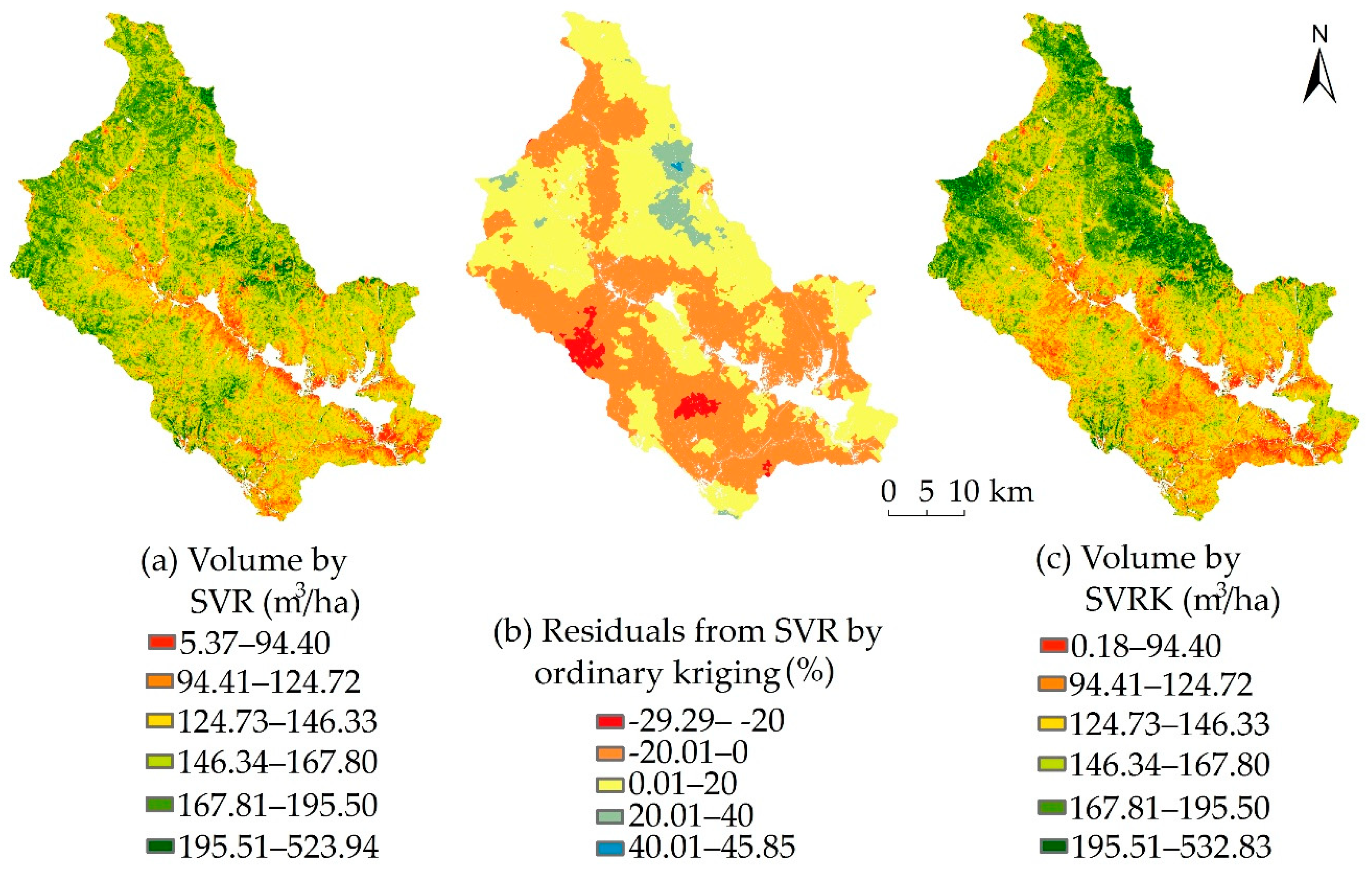
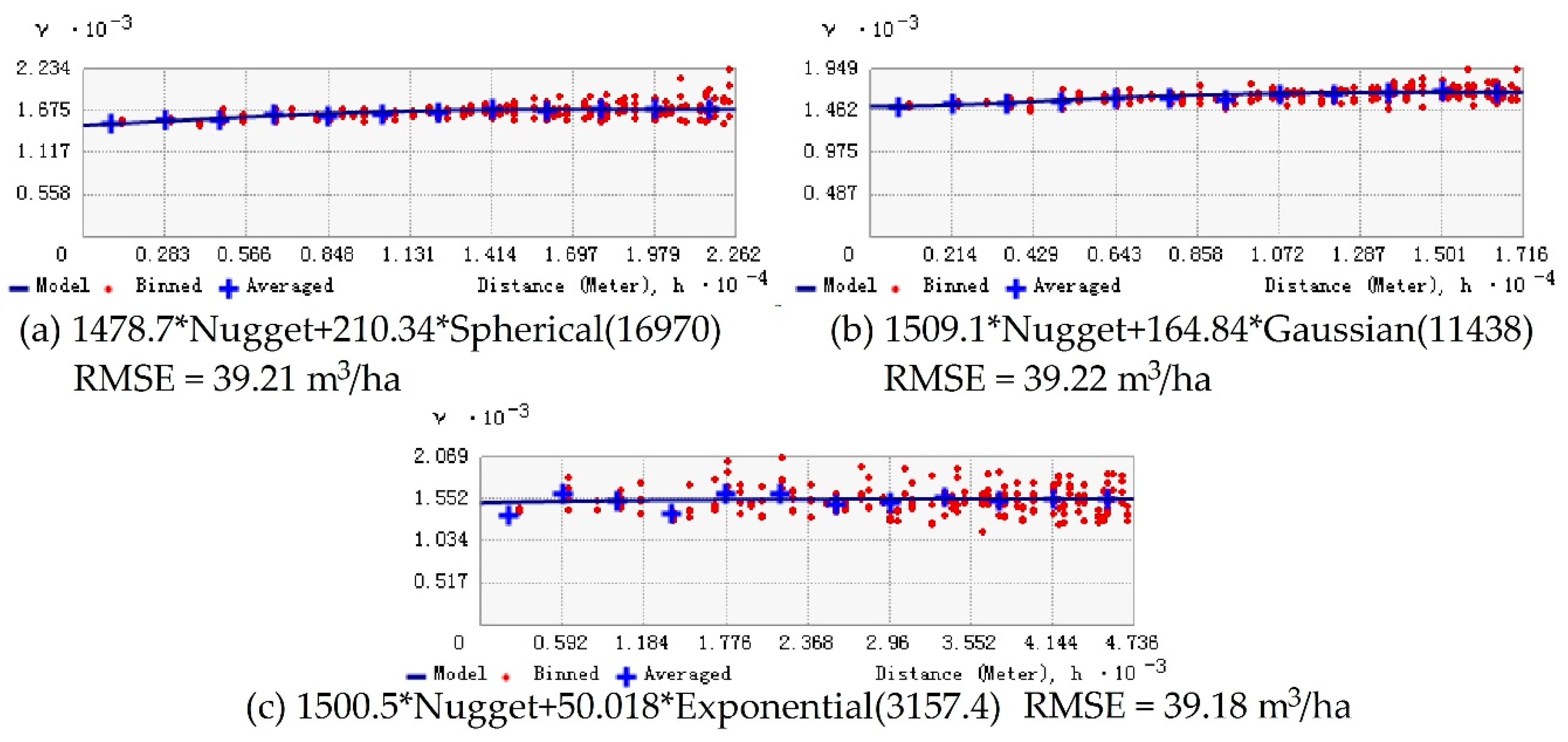
3.2.2. Integration of SVR Prediction and its Residuals by Ordinary Kriging

The residuals were calculated by the field-measured volume and SVR predicted values based on training data. The result of K-S showed that volume residuals from the SVR model possessed a normal distribution (p < 0.05), which could be used to calculate experimental semivariograms for ordinary kriging interpolation (Figure 6). Nugget values of spherical, Gaussian, and exponential models were 1478.7, 1509.1, and 1500.5, respectively. Range values were 16.97, 11.44, and 3.16 km, respectively. Sill values were 1689.04, 1673.94, and 1550.52, respectively. The strongest spatial autocorrelation is shown in the spherical model with the largest values of sill relative to nugget. While, the exponential model of ordinary kriging in Figure 6c was chosen to interpolate residuals from SVR with smallest RMSE 39.18 m3/ha. Based on Equation (2), the SVRK model was built.
By the optimal ordinary kriging model (Figure 6c), the distribution of volume residuals from the SVR model were obtained (Figure 5b). The interpolated values of volume residuals ranged from –29.29 to 45.85% (–42.79 to 66.99 m3/ha), with the mean and SD of 0.74 and 14.56 m3/ha, respectively. It was demonstrated that the overestimation of small volume values was located in the western and southern parts of the study area with residuals ranging from –29.29% to –20%. While the SVR model underestimated large volume values in the northern part of the study area, and residuals were from 40.01% to 45.85%.

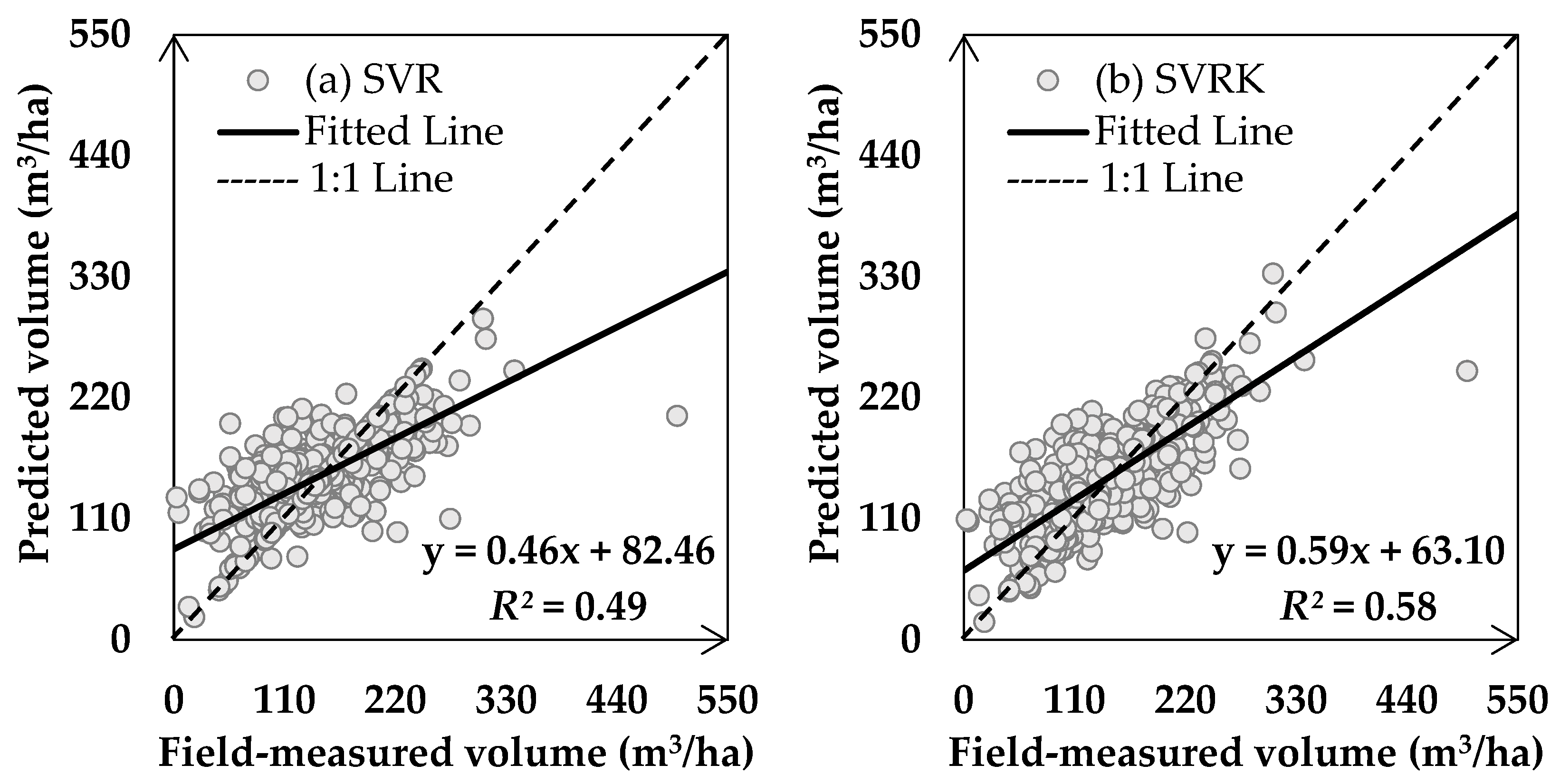
3.3. Models Assessment and Volume Mapping

Table 4 presented the accuracy of the SVR and SVRK models for estimating volume of the validation set (n = 464). The comparison of SVR and SVRK models demonstrated that additional prediction of residuals by ordinary kriging as the spatial autocorrelation, was more accurate than only considering influences of predictor variables from multi-sensor satellite data (Figure 7). It was indicated by ME values that both two models overestimated stand volume. SVRK remarkably improved accuracy of volume prediction over SVR by 9% (3.77 m3/ha) based on RMSE values.
The distribution of forest volume based on the SVRK model was acquired by combing the Figure 5a,b as the Figure 5c. By the optimal SVRK model, the predicted values of stand volume in the study area ranged from 0.18 to 532.83 m3/ha, with the mean and SD of 150.99 and 30.83 m3/ha, respectively (Figure 5c). Based on SVRK mapping, the northern part of the study area with high altitude had the largest volume values ranging from 195.51 to 532.83 m3/ha. In the south with low altitude and nearby the non-forest area, the smallest volume values ranged from 0.18 to 94.40 m3/ha. The map showed different distribution of stand volume with the SVR result, while values remained similar (Figure 5a,c). The six levels of stand volume in the SVRK map covered relatively equal areas than that in the SVR result, especially the largest (≥ 195.91 m3/ha). It was illustrated that the error, which was caused by the SVR model with the overestimation of small values and underestimation of large volume, was reduced. Forest volume of the SVRK map showed the greater spatial variation than that of the SVR. Namely, combining interpolation values of residuals, the spatial distribution of forest volume was much closer to the measured data (SD = 56.2 m3/ha).

4. Discussion

4.1. Multi-Sensor Satellite Predictors of Forest Volume Mapping

The role of multi-sensor variables on volume mapping was revealed by correlation coefficients (Table 3) and importance (Figure 4). SAR was able to penetrate forest canopy to a certain depth, and related to roughness and water content of vegetation [71], so that its variables were valuable for volume prediction. The elevation as a proxy of InSAR height, was dominant in volume prediction of this study. It was support from previous findings that InSAR height and its slope parameter were directly proportional to volume [72,73]. It was found that HV was more contributive to stand volume prediction than HH and VV channel; yet, VH backscatter was not significantly related. It was owing to the stronger sensitivity of HV backscatter to the forest growth stage than the HH and VV polarizations [74,75]. All backscatters showed positive relationships with volume. This was likely due to an increase in the volume of scattering with the growth of trees [76].
The penetrability was weaker with shorter wavelength. It resulted in the weaker capability of C band SAR for volume prediction than that of L band SAR according to our findings. It also revealed saturation problems of backscatters. The measured forest volume values in the study area were partially above 200 Mg/ha (Figure 2a), which were larger than the common saturation value of C band and smaller than that of L band SAR backscatters [48,77]. The results indicated that texture features of SAR data were much more helpful than original backscatters to forest volume prediction, which was consistent with existing researches [52,78]. However, textural indices from Sentinel-1 was marginal in this study for volume mapping compared to the previous finding [79]. It was resulted from the decrease in the heterogeneity by texture analysis and large variations of stand volume in the study area.
As optical sensor data, MSI variables, i.e., reflectance and spectral indices, were powerful for the retrieval of horizontal forest structures such as vegetation types, canopy cover and DBH [80,81]. Results revealed that the short-wave infrared (SWIR) band was the highly ranked variable for predicting stand volume. It was explained by the closer relationship between SWIR spectral band and vegetation properties, i.e., canopy biomass and water content, compared to other electromagnetic spectrum regions [82]. In line with existing studies, reflectance of optical bands and spectral indices were quite helpful in volume prediction [83,84], whereas, the role of red-edge bands and their vegetation indices in this study was minor than that in previous researches [58,85]. This may be caused by the diversity of tree species in the study area with different responses to various red-edge bands, the average relationships of which were weaker. In a word, topographic indices from L band InSAR, backscatters of L band SAR, texture features of VV channel from C band SAR and vegetation indices of MSI were recommended for stand volume mapping based on open-access satellite data in the heterogeneous temperate forests.

4.2. SVR versus SVRK

It was a pioneering study that built the SVRK hybrid model and utilized it to map stand volume. The optimal RBF-kernel SVR model trained in this study as the first step achieved higher accuracy than multiple linear regressions and SVR models with various kernels based on similar multi-sensor satellite data [31,32], while the SVR model in this study was less accurate than that built by ALOS optical and SAR variables [20]. It was attributed to coarser spatial resolution of L band SAR data and the complex composition of tree species in the study area. Moreover, the density of training dataset of this study (928 samples/171450 ha) was quite smaller than that of the reported research (77 samples/83.71 ha).
Results demonstrated that SVRK improved the mapping accuracy by incorporating interpolation values of residuals to SVR models (Figure 5 and Table 4). The value of the accuracy improvement of SVRK was smaller than that of RFK and ANNK for soil carbon prediction as reported [86,87,88]. It was resulted from the weaker autocorrelation of residuals from SVR compared with that of soil attributes, as well as the smaller sampling density. It was denoted that stand volume was influenced more by multi-sensor variables, and values of nearby sites affected less. The autocorrelation of volume residuals from SVR was weaker than that of biomass errors from RF, while the accuracy improvement of SVRK (RI = 0.09) for volume mapping was much more than that of RFK (RI = 0.07) for biomass prediction [25]. This is due to the higher spatial heterogeneity and the smaller training dataset of this study. The study concluded that SVRK was a promising approach for mapping stand volume with a small training dataset in heterogeneous temperate forests.

4.3. Spatial Variations of Stand Volume and Forest Management

The spatial distribution of forest volume derived by SVRK with more equal area of each level than the result of the commonly used SVR model was much closer to the measured data (Figure 2 and Figure 5a,c). Whereas, the stand volume map (SD = 30.83 m3/ha) displayed smaller spatial variations than measured data (SD = 56.2 m3/ha). The large variations of measured values of stand volume was resulted from the positively skew distribution with the majority below 300 m3/ha (Figure 2b). The maximum measured volume of 499.84 m3/ha belonged to a mature Pinus koraiensis (Sieb. et Zucc.) dominant natural forest site in the northern part of the study area. The smaller variations of SVRK-derived volume mainly resulted from the coarse mapping resolution as 30 m in this highly heterogeneous forest landscape. The smallest and largest levels of stand volume (< 94.90 and > 195.51 m3/ha) still occupied smaller areas than other four levels. It was illustrated that 30-m multi-sensor data from mosaic L band SAR and InSAR, C band SAR and MSI displayed a saturation problem in detecting small and large values of stand volume.
The volume values of different forest ages were summarized as Table 5 from the SVRK prediction by multi-sensor satellite data. Based on spatial and age variations of stand volume, certain measures can be taken for the sustainable forest management. In young forests, minimum, maximum and mean were all the smallest among five classes, while the variation was largest. The larger values of stand volume in young forests was mainly attributed to the high stand density. With tree growth, more space and resource competition occur among individual trees. Thus, young forests with volume above 195.51 m3/ha should be the critical focus areas, which need thinning (Figure 5c). However, the young forests with volume below 94.90 m3/ha should be enclosed for cultivation. The volume variation of middle-age forests was second-largest. Middle-age forests with volume above 195.51 m3/ha also require thinning, while the increment felling should be conducted in smaller volume areas. Near-mature forests obtained the smallest maximum of stand volume. Management measures in these forests can include the artificial promotion of natural regeneration and beforehand regeneration. Forest manager can selectively cut weak, pest-infested, and diseased trees in mature and over-mature forests.

5. Conclusions

Machine learning modeling with remote sensing data combined sample plot data has become a well adopted method to generate spatially explicit estimates of forest parameters. Among that, SVR has achieved wide success in application and has been praised for its ability to deal with small training datasets. A major shortcoming of machine learning is that it ignores the spatial autocorrelation of neighboring observed data. The main objective of the study was to build a hybrid model, i.e., SVRK, which integrated SVR and its residuals by ordinary kriging, based on a small training dataset. Then SVRK was used to map stand volume, the most common forest parameter needed for sustainable forest management at all scales. This study also determined the potential of open-access satellite predictors from multi-frequency SAR data in predicting volume in the heterogeneous temperate forests. As the first exploration of the SVRK modeling, this study provides an informative foundation for decision makers and other researchers on stand volume mapping with limited samples in northeastern China.
Based on the results of this study, the following was concluded:
(1)
SVRK can accurately predict stand volume of the heterogeneous Changbai Mountains Mixed forests with RMSE of 25.3% based on the low sampling density of 928 samples/171,450 ha, which improved accuracy of 9% than SVR.
(2)
Topographic indices from ALOS DSM as L band InSAR, backscatters of ALOS-2 as L band SAR, and texture features of VV channel from Sentinel-1 as C band SAR, as well as vegetation indices of Sentinel-2 MSI as the optical sensor were vital for explaining the observed variability of stand volume.
(3)
The northern part of the study area with high altitude had the largest volume values ranging from 195.51 to 532.83 m3/ha. In the south with low altitude and near a non-forest area, the smallest volume values ranged from 0.18 to 94.40 m3/ha.
(4)
Yong forests should be paid attention to and certain measures can be taken for sustainable forest management. Indeed, young forests with large volume need thinning, while that with small values should be enclosed for cultivation.

Author Contributions

L.C., C.R., and B.Z. designed this research. L.C. and C.R. conducted field sampling. L.C. performed the experiments, conducted the analysis, and drafted the manuscript. L.C., C.R., B.Z., and Z.W. revised and finalized the manuscript. All authors have read and agreed to the published version of the manuscript.

Funding

This study was supported by the National Key Research and Development Project of China (No. 2016YFC0500300), the Jilin Scientific and Technological Development Program (No. 20170301001NY), the funding from Youth Innovation Promotion Association of Chinese Academy of Sciences (No. 2017277, 2012178), and National Earth System Science Data Center of China.

Acknowledgments

The authors are grateful to the support from colleagues and local forestry bureau who participated in the field surveys and data collection. We thank the National Earth System Science Data Center (http://www.geodata.cn) for providing geographic information data. This study is supported by the National Key Research and Development Project of China (No. 2016YFC0500300), the Jilin Scientific and Technological Development Program (No. 20170301001NY), funding from Youth Innovation Promotion Association of Chinese Academy of Sciences (No. 2017277, 2012178), and National Earth System Science Data Center of China.

Conflicts of Interest

The authors declare no conflict of interest.

References

  1. Dube, T.; Sibanda, M.; Shoko, C.; Mutanga, O. Stand-volume estimation from multi-source data for coppiced and high forest Eucalyptus Spp. silvicultural systems in KwaZulu-Natal, South Africa. ISPRS J. Photogramm. Remote Sens. 2017, 132, 162–169. [Google Scholar] [CrossRef]
  2. Chirici, G.; Mura, M.; McInerney, D.; Py, N.; Tomppo, E.O.; Waser, L.T.; Travaglini, D.; McRoberts, R.E. A meta-analysis and review of the literature on the k-nearest neighbors technique for forestry applications that use remotely sensed data. Remote Sens. Environ. 2016, 176, 282–294. [Google Scholar] [CrossRef]
  3. Boisvenue, C.; Smiley, B.P.; White, J.C.; Kurz, W.A.; Wulder, M.A. Integration of Landsat time series and field plots for forest productivity estimates in decision support models. For. Ecol. Manag. 2016, 376, 284–297. [Google Scholar] [CrossRef]
  4. Lehmann, E.A.; Caccetta, P.; Lowell, K.; Mitchell, A.; Zhou, Z.S.; Held, A.; Milne, T.; Tapley, I. SAR and optical remote sensing: Assessment of complementarity and interoperability in the context of a large-scale operational forest monitoring system. Remote Sens. Environ. 2015, 156, 335–348. [Google Scholar] [CrossRef]
  5. Main, R.; Mathieu, R.; Kleynhans, W.; Wessels, K.; Naidoo, L. Hyper-temporal C Band SAR for baseline woody structural assessments in deciduous savannas. Remote Sens. 2016, 8, 661. [Google Scholar] [CrossRef] [Green Version]
  6. Chen, G.; Hay, G.J.; St-Onge, B. A GEOBIA framework to estimate forest parameters from lidar transects, Quickbird imagery and machine learning: A case study in Quebec, Canada. Int. J. Appl. Earth Obs. Geoinf. 2012, 15, 28–37. [Google Scholar] [CrossRef]
  7. Viana, H.; Aranha, J.; Lopes, O.; Cohen, W.B. Estimation of crown biomass of Pinus pinaster stands and shrubland above-ground biomass using forest inventory data, remotely sensed imagery and spatial prediction models. Ecol. Model. 2012, 226, 22–35. [Google Scholar] [CrossRef]
  8. Santoro, M.; Wegmüller, U.; Askne, J. Forest stem volume estimation using C-band interferometric SAR coherence data of the ERS-1 mission 3-days repeat-interval phase. Remote Sens. Environ. 2018, 216, 684–696. [Google Scholar] [CrossRef]
  9. Roy, A.; Royer, A.; Wigneron, J.-P.; Langlois, A.; Bergeron, J.; Cliche, P. A simple parameterization for a boreal forest radiative transfer model at microwave frequencies. Remote Sens. Environ. 2012, 124, 371–383. [Google Scholar] [CrossRef]
  10. Sharma, R.C.; Kajiwara, K.; Honda, Y. Estimation of forest canopy structural parameters using kernel-driven bi-directional reflectance model based multi-angular vegetation indices. ISPRS J. Photogramm. Remote Sens. 2013, 78, 50–57. [Google Scholar] [CrossRef]
  11. Alrababah, M.A.; Alhamad, M.N.; Bataineh, A.L.; Bataineh, M.N.; Suwaileh, A.F. Estimating east Mediterranean forest parameters using Landsat ETM. Int. J. Remote Sens. 2011, 32, 1561–1574. [Google Scholar] [CrossRef]
  12. Nilsson, M.; Nordkvist, K.; Jonzén, J.; Lindgren, N.; Axensten, P.; Wallerman, J.; Egberth, M.; Larsson, S.; Nilsson, L.; Eriksson, J.; et al. A nationwide forest attribute map of Sweden predicted using airborne laser scanning data and field data from the National Forest Inventory. Remote Sens. Environ. 2017, 194, 447–454. [Google Scholar] [CrossRef]
  13. Leboeuf, A.; Fournier, R.A.; Luther, J.E.; Beaudoin, A.; Guindon, L. Forest attribute estimation of northeastern Canadian forests using QuickBird imagery and a shadow fraction method. For. Ecol. Manag. 2012, 266, 66–74. [Google Scholar] [CrossRef]
  14. Abdullahi, S.; Kugler, F.; Pretzsch, H. Prediction of stem volume in complex temperate forest stands using TanDEM-X SAR data. Remote Sens. Environ. 2016, 174, 197–211. [Google Scholar] [CrossRef]
  15. Tamm, T.; Remm, K. Estimating the parameters of forest inventory using machine learning and the reduction of remote sensing features. Int. J. Appl. Earth Obs. Geoinf. 2009, 11, 290–297. [Google Scholar] [CrossRef]
  16. Wang, M.J.; Sun, R.; Xiao, Z.Q. Estimation of forest canopy height and aboveground biomass from spaceborne LiDAR and Landsat imageries in Maryland. Remote Sens. 2018, 10, 344. [Google Scholar] [CrossRef] [Green Version]
  17. Pal, M.; Mather, P.M. Support vector machines for classification in remote sensing. Int. J. Remote Sens. 2005, 26, 1007–1011. [Google Scholar] [CrossRef]
  18. Mountrakis, G.; Im, G.; Ogole, C. Support vector machines in remote sensing: A review. ISPRS J. Photogramm. Remote Sens. 2011, 66, 247–259. [Google Scholar] [CrossRef]
  19. dos Reis, A.A.; Carvalho, M.C.; de Mello, J.M.; Gomide, L.R.; Ferraz Filho, A.C.; Acerbi, F.W. Spatial prediction of basal area and volume in Eucalyptus stands using Landsat TM data: An assessment of prediction methods. N. Z. J. For. Sci. 2018, 48, 1. [Google Scholar] [CrossRef] [Green Version]
  20. de Souza, G.S.A.; Soares, V.P.; Leite, H.G.; Gleriani, J.M.; do Amaral, C.H.; Ferraz, A.S.; de Freitas Silveira, M.V.; dos Santos, J.F.C.; Silveira Velloso, S.G.; Domingues, G.F.; et al. Multi-sensor prediction of Eucalyptus stand volume: A support vector approach. ISPRS J. Photogramm. Remote Sens. 2019, 156, 135–146. [Google Scholar] [CrossRef]
  21. Kumar, S.; Lai, R.; Liu, D.S. A geographically weighted regression kriging approach for mapping soil organic carbon stock. Geoderma 2012, 189–190, 627–634. [Google Scholar] [CrossRef]
  22. Viscarra Rossel, R.A.; Webster, R.; Kidd, D. Mapping gamma radiation and its uncertainty from weathering products in a Tasmanian landscape with a proximal sensor and random forest kriging. Earth Surf. Proc. Land. 2013, 39, 735–748. [Google Scholar] [CrossRef]
  23. Tarasov, D.A.; Buevich, A.G.; Sergeev, A.P.; Shichkin, A.V. High variation topsoil pollution forecasting in the Russian Subarctic: Using artificial neural networks combined with residual kriging. Appl. Geochem. 2018, 88, 188–197. [Google Scholar] [CrossRef]
  24. Meng, Q.M.; Cieszewski, C.; Madden, M. Large area forest inventory using Landsat ETM+: A geostatistical approach. ISPRS J. Photogramm. Remote Sens. 2009, 64, 27–36. [Google Scholar] [CrossRef]
  25. Chen, L.; Wang, Y.Q.; Ren, C.Y.; Zhang, B.; Wang, Z.M. Assessment of multi-wavelength SAR and multispectral instrument data for forest aboveground biomass mapping using random forest kriging. For. Ecol. Manag. 2019, 447, 12–25. [Google Scholar] [CrossRef]
  26. Fayad, I.; Baghdadi, N.; Bailly, J.S.; Barbier, N.; Gond, V.; Hérault, B.; Hajj, M.E.; Fabre, F.; Perrin, J. Regional scale rain-forest height mapping using regression-kriging of spaceborne and airborne LiDAR data: Application on French Guiana. Remote Sens. 2016, 8, 240. [Google Scholar] [CrossRef] [Green Version]
  27. Li, Q.Q.; Zhang, X.; Wang, C.Q.; Li, B.; Gao, X.S.; Yuan, D.G.; Luo, Y.L. Spatial prediction of soil nutrient in a hilly area using artificial neural network model combined with kriging. Arch. Agron. Soil Sci. 2016, 62, 1541–1553. [Google Scholar] [CrossRef]
  28. Fazakas, Z.; Nilsson, M.; Olsson, H. Regional forest biomass and wood volume estimation using satellite data and ancillary data. Agric. For. Meteorol. 1999, 98–99, 417–425. [Google Scholar] [CrossRef]
  29. Wilhelm, S.; Hüttich, C.; Korets, M.; Schmullius, C. Large area mapping of boreal growing stock volume on an annual and multi-temporal level using PALSAR L-band backscatter mosaics. Forests 2014, 5, 1990–2015. [Google Scholar] [CrossRef] [Green Version]
  30. Chrysafis, I.; Mallinis, G.; Tsakiri, M.; Patias, P. Evaluation of single-date and multi-seasonal spatial and spectral information of Sentinel-2 imagery to assess growing stock volume of a Mediterranean forest. Int. J. Appl. Earth Obs. Geoinf. 2019, 77, 1–14. [Google Scholar] [CrossRef]
  31. Ataee, M.S.; Maghsoudi, Y.; Latifi, H.; Fadaie, F. Improving estimation accuracy of growing stock by multi-frequency SAR and multi-spectral data over Iran’s heterogeneously-structured broadleaf Hyrcanian forests. Forests 2019, 10, 641. [Google Scholar] [CrossRef] [Green Version]
  32. Mauya, E.W.; Koskinen, J.; Tegel, K.; Hämäläinen, J.; Kauranne, T.; Käyhkö, N. Modelling and predicting the growing stock volume in small-scale plantation forests of Tanzania using multi-sensor image synergy. Forests 2019, 10, 279. [Google Scholar] [CrossRef] [Green Version]
  33. Peregon, A.; Yamagata, Y. The use of ALOS/PALSAR backscatter to estimate above-ground forest biomass: A case study in Western Siberia. Remote Sens. Environ. 2013, 137, 139–146. [Google Scholar] [CrossRef]
  34. Reiche, J.; Lucas, R.; Mitchell, A.L.; Verbesselt, J.; Hoekman, D.H.; Haarpaintner, J.; Kellndorfer, J.M.; Rosenqvist, A.; Lehmann, E.A.; Woodcock, C.E.; et al. Combining satellite data for better tropical forest monitoring. Nat. Clim. Chang. 2016, 6, 120–122. [Google Scholar] [CrossRef]
  35. Chowdhury, T.A.; Thiel, C.; Schmullius, C. Growing stock volume estimation from L-band ALOS PALSAR polarimetric coherence in Siberian forest. Remote Sens. Environ. 2014, 155, 129–144. [Google Scholar] [CrossRef]
  36. Santoro, M.; Cartus, O.; Fransson, J.E.S.; Wegmüller, U. Complementarity of X-, C-, and L-band SAR backscatter observations to retrieve forest stem volume in boreal forest. Remote Sens. 2019, 11, 1563. [Google Scholar] [CrossRef] [Green Version]
  37. Stage, A.R.; Salas, C. Interactions of elevation, aspect, and slope in models of forest species composition and productivity. For. Sci. 2007, 53, 486–492. [Google Scholar]
  38. Rahlf, J.; Breidenbach, J.; Solberg, S.; Næsset, E.; Astrup, R. Comparison of four types of 3D data for timber volume estimation. Remote Sens. Environ. 2014, 155, 325–333. [Google Scholar] [CrossRef]
  39. Tadono, T.; Takaku, J.; Tsutsui, K.; Oda, F.; Nagai, H. Status of “ALOS World 3D (AW3D)” global DSM generation. In Proceedings of the 2015 IEEE International Geoscience and Remote Sensing Symposium (IGARSS), Milan, Italy, 26–31 July 2015. [Google Scholar]
  40. Xu, C.; Manley, B.; Morgenroth, J. Evaluation of modelling approaches in predicting forest volume and stand age for small-scale plantation forests in New Zealand with RapidEye and LiDAR. Int. J. Appl. Earth Obs. Geoinf. 2018, 73, 386–396. [Google Scholar] [CrossRef]
  41. Schumacher, J.; Rattay, M.; Kirchhöfer, M.; Adler, P.; Kändler, G. Combination of multi-temporal sentinel 2 images and aerial image based canopy height models for timber volume modelling. Forests 2019, 10, 746. [Google Scholar] [CrossRef] [Green Version]
  42. Olson, D.M.; Dinerstein, E.; Wikramanayake, E.D.; Burgess, N.D.; Powell, G.V.N.; Underwood, E.C.; D’Amico, J.A.; Itoua, I.; Strand, H.E.; Morrison, J.C.; et al. Terrestrial ecoregions of the world: A new map of life on Earth. Bioscience 2001, 51, 933–938. [Google Scholar] [CrossRef]
  43. Wang, Y.Q.; Wu, Z.F.; Yuan, X.; Zhang, H.Y.; Zhang, J.Q.; Xu, J.W.; Lu, Z.; Zhou, Y.Y.; Feng, J. Resources and ecological security of the Changbai Mountain region in Northeast Asia. In Remote Sensing of Protected Lands; Wang, Y.Q., Ed.; CRC Press: Boca Raton, FL, USA, 2011. [Google Scholar]
  44. Cai, H.Y.; Di, X.Y.; Chang, S.X.; Wang, C.K.; Shi, B.K.; Geng, P.F.; Jin, G.Z. Carbon storage, net primary production, and net ecosystem production in four major temperate forest types in northeastern China. Can. J. For. Res. 2016, 45, 143–151. [Google Scholar] [CrossRef]
  45. Ma, J.; Xiao, X.M.; Qin, Y.W.; Chen, B.Q.; Hu, Y.M.; Li, X.P.; Zhao, B. Estimating aboveground biomass of broadleaf, needleleaf, and mixed forests in Northeastern China through analysis of 25-m ALOS/PALSAR mosaic data. For. Ecol. Manag. 2017, 389, 199–210. [Google Scholar] [CrossRef]
  46. MOF (Ministry of Forestry). Standards for Forestry Resource Survey; China Forestry Publisher: Beijing, China, 1982. [Google Scholar]
  47. Forestry Administration of China. Tree Volume Tables (National Standard # LY/T 1353-1999); Forestry Administration of China: Beijing, China, 1999. [Google Scholar]
  48. Santi, E.; Paloscia, S.; Pettinato, S.; Chirici, G.; Mura, M.; Maselli, F. Application of neural networks for the retrieval of forest woody volume from SAR multifrequency data at L and C bands. Eur. J. Remote Sens. 2015, 48, 673–687. [Google Scholar] [CrossRef] [Green Version]
  49. Urbazaev, M.; Cremer, F.; Migliavacca, M.; Reichstein, M.; Schmullius, C.; Thiel, C. Potential of multi-temporal ALOS-2 PALSAR-2 ScanSAR data for vegetation height estimation in tropical forests of Mexico. Remote Sens. 2018, 10, 1227. [Google Scholar] [CrossRef] [Green Version]
  50. Shimada, M.; Isoguchi, O.; Tadono, T.; Isono, K. PALSAR radiometric and geometric calibration. IEEE Trans. Geosci. Remote Sens. 2009, 47, 3915–3932. [Google Scholar] [CrossRef]
  51. Sentinel-1_Team. Sentinel-1 User Handbook; European Space Agency: Paris, France, 2013. [Google Scholar]
  52. Dos Reis, A.A.; Franklin, S.E.; de Mello, J.M.; Junior, F.W.A. Volume estimation in a Eucalyptus plantation using multi-source remote sensing and digital terrain data: A case study in Minas Gerais State, Brazil. Int. J. Remote Sens. 2019, 4, 2683–2702. [Google Scholar] [CrossRef]
  53. Veci, L. Sentinel-1 Toolbox: SAR Basics Tutorial; ARRAY Systems Computing, Inc.: Toronto, ON, Canada; European Space Agency: Paris, France, 2015. [Google Scholar]
  54. Laurin, G.V.; Balling, J.; Corona, P.; Mattioli, W.; Papale, D.; Puletti, N.; Rizzo, M.; Truckenbrodt, J.; Urban, M. Above-ground biomass prediction by Sentinel-1 multitemporal data in central Italy with integration of ALOS2 and Sentinel-2 data. J. Appl. Remote Sens. 2018, 12, 016008. [Google Scholar] [CrossRef]
  55. Sentinel-2_Team. Sentinel-2 User Handbook; European Space Agency: Paris, France, 2015. [Google Scholar]
  56. Puliti, S.; Saarela, S.; Gobakken, T.; Ståhl, G.; Naesset, E. Combining UAV and Sentinel-2 auxiliary data for forest growing stock volume estimation through hierarchical model-based inference. Remote Sens. Environ. 2018, 204, 485–497. [Google Scholar] [CrossRef]
  57. Astola, H.; Häme, T.; Sirro, L.; Molinier, M.; Kilpi, J. Comparison of Sentinel-2 and Landsat 8 imagery for forest variable prediction in boreal region. Remote Sens. Environ. 2019, 223, 257–273. [Google Scholar] [CrossRef]
  58. Chrysafis, I.; Mallinis, G.; Siachalou, S.; Patias, P. Assessing the relationships between growing stock volume and Sentinel-2 imagery in a Mediterranean forest ecosystem. Remote Sens. Lett. 2017, 8, 508–517. [Google Scholar] [CrossRef]
  59. Wittke, S.; Yu, X.W.; Karjalainen, M.; Hyyppä, J.; Puttonen, E. Comparison of two-dimensional multitemporal Sentinel-2 data with three dimensional remote sensing data sources for forest inventory parameter estimation over a boreal forest. Int. J. Appl. Earth Obs. Geoinf. 2019, 76, 167–178. [Google Scholar] [CrossRef]
  60. Wijaya, A.; Kusnadi, S.; Gloaguen, R.; Heilmeier, H. Improved strategy for estimating stem volume and forest biomass using moderate resolution remote sensing data and GIS. J. For. Res. 2010, 21, 1–12. [Google Scholar] [CrossRef]
  61. Chen, L.; Wang, Y.Q.; Ren, C.Y.; Zhang, B.; Wang, Z.M. Optimal combination of predictors and algorithms for forest above-ground biomass mapping from Sentinel and SRTM data. Remote Sens. 2019, 11, 414. [Google Scholar] [CrossRef] [Green Version]
  62. Xu, L.; Shi, Y.J.; Fang, H.Y.; Zhou, G.M.; Xu, X.J.; Zhou, Y.F.; Tao, J.X.; Ji, B.Y.; Xu, J.; Li, C.; et al. Vegetation carbon stocks driven by canopy density and forest age in subtropical forest ecosystems. Sci. Total Environ. 2018, 631–632, 619–626. [Google Scholar] [CrossRef]
  63. Gunn, S.R. Support Vector Machines for Classification and Regression; Technical Report; University of Southampton: Southampton, UK, 1998. [Google Scholar]
  64. Williams, G. Data Mining with Rattle and R: The Art of Excavating Data for Knowledge Discovery, use R; Springer Science+Business Media, LLC: New York, NY, USA, 2011. [Google Scholar]
  65. Were, K.; Bui, D.T.; Dick, Ø.B.; Singh, B.R. A comparative assessment of support vector regression, artificial neural networks, and random forests for predicting and mapping soil organic carbon stocks across an Afromontane landscape. Ecol. Indic. 2015, 52, 394–403. [Google Scholar] [CrossRef]
  66. Platt, J. Fast Training of Support Vector Machines Using Sequential Minimal Optimization; MIT Press: Cambridge, MA, USA, 1999. [Google Scholar]
  67. Isaaks, E.H.; Srivastava, R.M. An Introduction to Applied Geostatistics; Oxford University Press: Oxford, England, 1989. [Google Scholar]
  68. Ou, Y.; Rousseau, A.N.; Wang, L.X.; Yan, B.X. Spatio-temporal patterns of soil organic carbon and pH in relation to environmental factors-A case study of the Black Soil Region of Northeastern China. Agric. Ecosyst. Environ. 2017, 245, 22–31. [Google Scholar] [CrossRef]
  69. Tang, G.A.; Yang, X. ArcGIS Experimental Course for Spatial Analysis, 2nd ed.; Science Press: Beijing, China, 2013. [Google Scholar]
  70. Chen, L.; Ren, C.Y.; Zhang, B.; Wang, Z.M.; Wang, Y.Q. Mapping spatial variations of structure and function parameters for forest condition assessment of the Changbai Mountain National Nature Reserve. Remote Sens. 2019, 11, 3004. [Google Scholar] [CrossRef] [Green Version]
  71. Lu, D.S.; Chen, Q.; Wang, G.X.; Liu, L.J.; Li, G.Y.; Moran, E. A survey of remote sensing-based aboveground biomass estimation methods in forest ecosystems. Int. J. Digit. Earth 2016, 9, 63–105. [Google Scholar] [CrossRef]
  72. Gama, F.F.; dos Santos, J.R.; Mura, J.C. Eucalyptus biomass and volume estimation using interferometric and polarimetric SAR data. Remote Sens. 2010, 2, 939–956. [Google Scholar] [CrossRef] [Green Version]
  73. Solberg, S.; Astrup, R.; Breidenbach, J.; Nilsen, B.; Weydahl, D. Monitoring spruce volume and biomass with InSAR data from TanDEM-X. Remote Sens. Environ. 2013, 139, 60–67. [Google Scholar] [CrossRef]
  74. Aslan, A.; Rahman, A.F.; Warren, M.W.; Robeson, S.W. Mapping spatial distribution and biomass of coastal wetland vegetation in Indonesian Papua by combining active and passive remotely sensed data. Remote Sens. Environ. 2016, 183, 65–81. [Google Scholar] [CrossRef]
  75. Sinha, S.; Santra, A.; Sharma, L.; Jeganathan, C.; Nathawat, M.S.; Das, A.K.; Mohan, S. Multi-polarized Radarsat-2 satellite sensor in assessing forest vigor from above ground biomass. J. For. Res. 2018, 29, 1139–1145. [Google Scholar] [CrossRef]
  76. Pham, T.D.; Yoshion, K. Aboveground biomass estimation of mangrove species using ALOS-2 PALSAR imagery in Hai Phong City, Vietnam. J. Appl. Remote Sens. 2017, 11, 026010. [Google Scholar] [CrossRef]
  77. Fransson, J.E.S.; Ispraelsson, H. Estimation of stem volume in boreal forests using ERS-1 C- an JERS-1 L-band SAR data. Int. J. Remote Sens. 1999, 20, 123–137. [Google Scholar] [CrossRef]
  78. Thiel, C.; Schmullius, C. The potential of ALOS PALSAR backscatter and InSAR coherence for forest growing stock volume estimation in Central Siberia. Remote Sens. Environ. 2016, 173, 258–273. [Google Scholar] [CrossRef]
  79. Morin, D.; Planells, M.; Guyon, D.; Villard, L.; Mermoz, S.; Bouvet, A.; Thevenon, H.; Dejoux, J.-F.; Toan, T.L.; Dedieu, G. Estimation and mapping of forest structure parameters from open access satellite images: Development of a generic method with a study case on coniferous plantation. Remote Sens. 2019, 11, 1275. [Google Scholar] [CrossRef] [Green Version]
  80. Peña, M.A.; Brenning, A.; Sagredo, A. Constructing satellite-derived hyperspectral indices sensitive to canopy structure variables of a Cordilleran Cypress (Austrocedrus chilensis) forest. ISPRS J. Photogramm. Remote Sens. 2012, 74, 1–10. [Google Scholar] [CrossRef]
  81. Lausch, A.; Erasmi, S.; King, D.J.; Magdon, P.; Heurich, M. Understanding forest health with remote sensing-part II—A review of approaches and data models. Remote Sens. 2017, 9, 129. [Google Scholar] [CrossRef] [Green Version]
  82. Dube, T.; Mutanga, O.; Abdel-Rahman, E.A.; Ismail, R.; Slotow, R. Predicting Eucalyptus spp. Stand volume in Zululand, South Africa: An analysis using a stochastic gradient boosting regression ensemble with multi-source data sets. Int. J. Remote Sens. 2015, 36, 3751–3772. [Google Scholar] [CrossRef]
  83. Latifi, H.; Nothdurft, A.; Koch, B. Non-parametric prediction and mapping of standing timber volume and biomass in a temperate forest: Application of multiple optical/LiDAR-derived predictors. Forestry 2010, 83, 395–407. [Google Scholar] [CrossRef] [Green Version]
  84. Mura, M.; Bottalico, F.; Giannetti, F.; Bertani, R.; Giannini, R.; Mancini, M.; Orlandini, S.; Travaglini, D.; Chiricia, G. Exploiting the capabilities of the Sentinel-2 multi spectral instrument for predicting growing stock volume in forest ecosystems. Int. J. Appl. Earth Obs. Geoinf. 2018, 66, 126–134. [Google Scholar] [CrossRef]
  85. Korhonen, L.; Packalen, H.P.; Rautiainen, M. Comparison of Sentinel-2 and Landsat 8 in the estimation of boreal forest canopy cover and leaf area index. Remote Sens. Environ. 2017, 195, 259–274. [Google Scholar] [CrossRef]
  86. Dai, F.Q.; Zhou, Q.G.; Lv, Z.Q.; Wang, X.M.; Liu, G.C. Spatial prediction of soil organic matter content integrating artificialneural network and ordinary kriging in Tibetan Platea. Ecol. Indic. 2014, 45, 184–194. [Google Scholar] [CrossRef]
  87. Guo, P.T.; Li, M.F.; Luo, W.; Tang, Q.F.; Liu, Z.W.; Lin, Z.M. Digital mapping of soil organic matter for rubber plantation at regional scale: An application of random forest plus residuals kriging approach. Geoderma 2015, 237–238, 49–59. [Google Scholar] [CrossRef]
  88. Tziachris, P.; Aschonitis, V.; Chatzistathis, T.; Papadopoulou, M. Assessment of spatial hybrid methods for predicting soil organic matter using DEM derivatives and soil parameters. Catena 2019, 174, 206–216. [Google Scholar] [CrossRef]
Figure 1. The outline of the study area, sampling sites, and employed open-access satellite remote sensing data derived from Advanced Land Observing Satellite (ALOS), ALOS-2, Sentinel-1, and Sentinel-2 series. Date include (a) Sentinel-2 Level-1C, (b) ALOS-2 yearly mosaic, (c) Sentinel-1 Level-1 GRD, (d) Sentinel-2 Level-2A, and (e) ALOS Digital Surface Model products.
Forests 11 00296 g001
Figure 2. The values of measured stand volume. (a) Field sample profiles of volume in the study site from Plot 1 to 1,392; (b) Components of volume.
Forests 11 00296 g002
Figure 3. Illustration of support vector machine for regression kriging (SVRK). It includes (a) the first step as the support vector machine for regression (SVR) algorithm and (b) the second step as the sum of SVR and residuals interpolated by ordinary kriging. I, Imean, and Isd are raw, mean and standard deviation values, respectively.
Forests 11 00296 g003
Figure 4. Variable importance shown by increase in the root mean square errors (RMSEs) of SVR models after excluding a predictor.
Forests 11 00296 g004
Figure 5. Stand volume mapping by SVR (a), and its residuals interpolated by ordinary kriging (%, divided by the mean measured value of stand volume) (b) as well as final prediction by SVRK (c).
Forests 11 00296 g005
Figure 6. Experimental variograms and fitted models of residuals from SVR by (a) spherical, (b) Gaussian, and (c) exponential models.
Forests 11 00296 g006
Figure 7. Scatter plots of predicted versus observed volume from validation data based on SVR (a) and SVRK (b) models.
Forests 11 00296 g007
Table 1. The adopted ALOS-2, Sentinel-1, Sentinel-2, and digital surface model (DSM) data.
SensorsElementsTimeSpatial Resolution (m)
ALOS-2N043E127/N043E128/
N044E127/N044E128
201725
Sentinel-1D633_FCEE of Sentinel-1B2017092710
Sentinel-2T52TCP/T52TCN of Sentinel-2A,2017092310
T52TDN of Sentinel-2B20170925
ALOSN042E127/N042E128/
N043E127/N043E128
Derived from PALSAR data during 2006 to 201130
Table 2. Remote sensing indices from the ALOS and Sentinel series data for volume mapping.
Source ImageRelevant VariablesDescription
ALOS-2
L band SAR
PolarizationHVNormalized backscatter coefficient of horizontal transmit-vertical channel in dB
HHNormalized backscatter coefficient of horizontal transmit-horizontal channel in dB
Sentinel-1
C band SAR
PolarizationVVNormalized backscatter coefficient of vertical transmit-vertical channel in dB
VHNormalized backscatter coefficient of vertical transmit-horizontal channel in dB
TextureVV/VH_CONContrast
VV/VH_DIS Dissimilarity
VV/VH_HOMHomogeneity
VV/VH_ASMAngular second moment
VV/VH_ENEEnergy
VV/VH_MAXMaximum probability
VV/VH_ENTEntropy
VV/VH_MEAGray-level co-occurrence matrix (GLCM) mean
VV/VH_VARGLCM variance
VV/VH_CORGLCM correlation
Sentinel-2
MSI
Multispectral bandsB2Blue, 490 nm
B3Green, 560 nm
B4Red, 665 nm
B5Red edge, 705 nm
B6Red edge, 749 nm
B7Red edge, 783 nm
B8Near infrared, 842 nm
B8aNear infrared, 865 nm
B11Short-wave infrared, 1610 nm
B12Short-wave infrared, 2190 nm
Vegetation indicesRVIRatio vegetation index, B8/B4
DVIDifference vegetation index, B8–B4
PVIPerpendicular vegetation index,
sin(45°)×B8–cos(45°)×B4
NDVINormalized difference vegetation index,
(B8 − B4)/(B8 + B4)
SAVISoil adjusted vegetation index,
1.5 × (B8 − B4)/(B8 + B4 + 0.5)
NDVI5Normalized difference vegetation index with bands 4 and 5, (B5 − B4)/(B5 + B4)
NLI5Non-linear vegetation index with bands 4 and 5,
(B52 − B4)/(B52 + B4)
NDVI6Normalized difference vegetation index with bands 4 and 6, (B6 − B4)/(B6 + B4)
NDVI7Normalized difference vegetation index with bands 4 and 7, (B7 − B4)/(B7 + B4)
NDVI8aNormalized difference vegetation index with bands 4 and 8a, (B8a − B4)/(B8a + B4)
MSIMoisture stress index, B8/B11
EVI5Enhanced vegetation index with bands 4, 5 and 2,
2.5 * (B5 − B4) / (B5 + 6 * B4 − 7.5 * B2 + 1)
S2REPSentinel-2 red-edge position index,
705 + 35 × [(B4 + B7)/2 − B5] × (B6 − B5)
Transform indicesTCWTasseled cap wetness, 0.1509 * B2 + 0.1973 * B3 + 0.3279 * B4 + 0.3406 * B8 + 0.7112 * B11 + 0.4572 * B12
TCBTasseled cap brightness, 0.3037 * B2 + 0.2793 * B3 + 0.4743 * B4 + 0.5585 * B8 + 0.5082 * B11 + 0.1863 * B12
TCGTasseled cap greenness, −0.2848 * B2 − 0.2435 * B3 − 0.5436 * B4 + 0.7243 * B8 + 0.0840 * B11 − 0.1800 * B12
ALOS
DSM
Topographic indicatorsHElevation
SSlope
AAspect
MSurface roughness
SPIStream power index, Ln[Ac × tanβ × 100]
Table 3. Related variables and predictors derived from multi-sensor satellite data for stand volume mapping. * denotes significance with a p-value of the t-test being below 0.05; ** denotes strong significance with a p-value below 0.01.
Source ImageRelated VariablesrCollinear WithPredictors
ALOS-2HV0.138 **/Yes
HH0.181 **/Yes
Sentinel-1VV0.075 **/Yes
VV_MEA0.090 **VV/VH_ VAR, VH_MEAYes
VV_VAR0.087 **VV/VH_MEA, VH_VARNo
VH_MEA0.057 *VV/VH_ VAR, VV_MEANo
VH_VAR0.061 *VV/VH_MEA, VV_VARNo
Sentinel-2B2−0.192 **/Yes
B3−0.111 **B5, TCWYes
B4−0.162 **/Yes
B5−0.079 **B3, B11, TCWNo
B11−0.111 **B5, B12, TCWNo
B12−0.145 **B11Yes
RVI0.145 **NDVI, NDVI5, NDVI6, NDVI7, NDVI8aNo
DVI0.087 **PVI, SAVI, TCG No
PVI0.087 **DVI, SAVI, TCG No
NDVI0.175 **RVI, NDVI5, NDVI6, NDVI7, NDVI8aYes
SAVI0.110 **DVI, PVI, TCGYes
NDVI50.151 **RVI, NDVI, NDVI6, NDVI7, NDVI8aNo
NLI50.065 */Yes
NDVI60.165 **RVI, NDVI5, NDVI, NDVI7, NDVI8aNo
NDVI70.166 **RVI, NDVI5, NDVI, NDVI6, NDVI8aNo
NDVI8a0.167 **RVI, NDVI5, NDVI, NDVI6, NDVI7No
MSI0.105 **/Yes
S2REP0.063 */Yes
TCW−0.074 **B3, B5, B11No
TCG0.087 **DVI, PVI, SAVINo
ALOS
DSM
H0.252 **/Yes
S0.154 **MYes
A0.091 **/Yes
M0.117 **SNo
Table 4. Accuracy assessment of stand volume modeling based on independent validation data.
ModelMERMSErRI
m3/ha%m3/ha%
SVR −4.49−3.0740.7327.880.70/
SVRK−3.9−2.6736.9625.300.760.09
Table 5. Stand volume of forests with different ages in the study area.
AgeMinimumMaximumMeanStandard DeviationCoefficient of Variation (%)
Yong0.18358.78134.7929.9122.19
Middle-age0.21520.56138.3029.7921.54
Near-mature1.18463.83152.5128.4718.67
Mature1.71532.83156.3830.0919.24
Over-mature7.91521.99160.4830.6419.09

