Abstract
The Comprehensive Commercial Logging Ban in All Natural Forests (CCLB) policy, introduced in April 2015, aims to protect all natural forests in China. It has impacted both China’s domestic timber supply and imports. We investigated price transmission in China’s hardwood lumber imports resulting from the implementation of this policy. We selected three hardwood lumber species, i.e., Sapelli (Entandrophragma), Mandshurica (Fraxinus), and Laurel (Terminalia), and used their daily prices from 30 April 2015 to 30 November 2017. Threshold co-integration and threshold error correction models are employed for this analysis. We identified a structural breakpoint on 30 November 2016, and consequently partitioned the data series into two parts for the two subperiods separated by the breakpoint. The empirical results indicated that there was asymmetric price transmission (APT) for both subperiods. Adjustment of positive price deviations to the long-term equilibrium levels was slower than that of negative price deviations. In the short term, the price of high-quality lumber evolved independently, whereas the price of lower-quality lumber tended to return to the equilibrium. The APT reflects a redistribution of welfare, benefiting the exporters more than the importers. We find that positive discrepancies in each price pair were inclined to be more persistent in the first subperiod than in the second subperiod. This could attribute to the fact that the degree of CCLB intervention in the former one was higher than in the latter one.
1. Introduction
China is heavily dependent on timber imports because of its limited forest resources [1,2]. China’s timber (logs and lumber) imports reached 97 million m3, valued at US $19.9 billion and accounting for 32% of all timber trade value worldwide in 2014 [3]. A sizable portion of China’s timber imports, especially in value, is hardwood imports, which reached approximately 29.8 million m3 (US $10.6 billion) in 2014. The import value of hardwood lumber alone reached US $4.3 billion in that year, accounting for 33% of the total global hardwood lumber trade [3] and making China the world’s largest importer of hardwood lumber.
To further protect its natural forests, China enacted the Comprehensive Commercial Logging Ban in Natural Forests (CCLB) on 1 April 2015. As a result, the major state-owned forests in Inner Mongolia, Liaoning, Jilin, and Heilongjiang ceased commercial logging completely. In 2016, all state forests suspended commercial logging activities. On 15 March 2017, the CCLB was implemented in all state, collective, and private natural forests. The effects have been remarkable. The timber harvest from natural forests was 5.27 million m3 in 2015, falling to 1.71 million m3 in 2016, and further to 1.26 million m3 in 2017 [4]. Given the immaturity of forest plantations, most domestic large-diameter hardwood came from natural forests [5,6,7]. Thus, China’s hardwood lumber imports soared by 16.38% (in volume) in 2016 and by another 10.61% in 2017 [3].
The CCLB is likely to trigger the asymmetric price transmission (APT) of imported hardwood lumber as well. APT reflects the inability of the market to respond similarly to positive and negative price disequilibria [8], usually because of policy interventions [9,10,11,12]. Faced with a major decline in timber production by natural forests, exporters are apt to believe that any price reduction in hardwood lumber imports would be temporary, and any price increase permanent. Exporters tend to respond slowly to positive price deviations from the long-term equilibrium, but comparatively act quickly to negative price deviations.
APT, a microeconomic concept [10] that has received increasing attention, can be divided into several types. For instance, there are positive and negative APTs. A positive APT indicates that an increase in price is transmitted more rapidly or completely than a decrease, while a negative APT indicates the opposite. APT can also be grouped into vertical and spatial components. The vertical APT refers to price transmission of a single product along the supply chain. The spatial APT indicates that prices are transmitted among congeneric products in the same region of an industrial chain.
APT has received growing attention in the past few decades [13]. In an extensive study of 282 products and product categories, Peltzman found asymmetric price transmission to be the rule rather than the exception [14]. The research objects of APT are mainly agricultural products [15,16,17,18,19,20,21,22]. Vertical APT is evident in the supply chains of many such products, including pork in Switzerland and U.S. [19,21], wild cod in France [11], imported salmon in Germany [20] and rice in Bangladesh [22]. Their conclusions were similar: downstream prices react more rapidly to disequilibria induced by upstream price increases than by upstream price decreases. On the contrary, for farmed salmon in France, the downstream retail price responded more slowly to rises than declines in upstream production prices, because the loss of the unit margin was offset by increased sales [11]. Spatial APT focuses on agriculture markets. Using a threshold co-integration framework, Abdulai demonstrated that local maize markets in Ghana responded more quickly to rising prices than to falling prices in the central markets [23]. Ganneval showed that if the price volatility of four commodities (rapeseed, corn, feed barley, and protein pea) was high in France, any price deviations from the long-term equilibrium were corrected rapidly; forward prices became more relevant as price volatility increased [24]. The study on APT of wheat exported from North America showed that USA enterprises exporting low-quality wheat may reduce prices faster (to maintain market share) than Canadian exporters of high-quality wheat [8,25]. The causes of APT (principally transaction costs and market forces) have also been explored extensively for agricultural products markets in Europe, Asia, and Africa [26,27,28,29,30].
APT is also detected in forest product markets. Vertical APT was evident in the Greek roundwood market; consumer prices adjusted more slowly to increases than to decreases in domestic producer prices [31]. The Korean fiberboard industry exhibited a reverse price adjustment that was vertically asymmetric; wholesale prices reacted more rapidly to rises than to fall in factory prices [32]. Similarly, vertical APT was evident in lumber supply chains for the southern and western USA, where prices were more responsive when price margins increased rather than decreased [33]. Sun showed that, in the USA, spatial price transmission of imported wooden beds (from China and Vietnam) was asymmetric, and that Vietnamese exporters aiming to meet the price of Chinese wooden beds responded faster to a price spread expansion than to a price spread contraction [34].
Although studies exploring asymmetry in agricultural product price adjustments have been extensive, few studies have addressed APT in the context of forest products. In particular, to the best of our knowledge, no report has yet evaluated the spatial APT of forest products after a policy intervention. Hence, we investigate the spatial APT of hardwood lumber imported by China in the era of the CCLB. We focus on three representative hardwood trees: Sapelli (Entandrophragma), Mandshurica (Fraxinus), and Laurel (Terminalia) (For all three species, the Latin names are given in parentheses. The English names used to describe the Terminalia differ in the countries of origin. “Laurel” is the name used in the leading exporting country (Myanmar)), because they are major hardwood lumber species imported by China and reflect different wood qualities and prices with similar end-uses. We examine their price dynamics and APT using threshold co-integration models and threshold error correction models (TECMs). We show that APT is evident in the market of China’s imported hardwood lumber after implementation of the CCLB. Our findings are informative for both policymakers, importers, and exporters while enriching the literature on forest products markets and trade.
2. Materials and Methods
2.1. Preliminary Analysis of Data
Sapelli, Mandshurica, and Laurel are the major hardwood lumber species imported by China. Sapelli is imported primarily from Africa, Mandshurica from Russia, and Laurel from Myanmar, Vietnam, and several African countries [35]. The import values of Mandshurica (US $291 million) and Sapelli (US $52 million) are the second-and fifth-largest among all species of hardwood lumber imported in 2016. Laurel has many subspecies, the trade indices of which are not distinguished in United Nations Comtrade. Given their superior properties, these three species are widely used to produce wooden furniture, floors, doors, and interior decorations, and they are substitutes in consumption. We obtained their price data from the China Timber Price Index Network of China’s Development and Reform Commission. The database provides daily price information on most timber trading markets in China. All price data were obtained from the Great Southwest Building Material Market in Sichuan, one of the largest timber markets in China. The daily price series were based on the price for the highest single-deal volume for that day. Freight and transportation costs were not included, and for the study period no tariff was imposed on imported lumber. The market prices of all three species, measured in Chinese yuan (CNY)/m3, were hierarchical (Figure 1). The average prices of Sapelli, Mandshurica, and Laurel over the study period were CNY6718 (US $1027)/m3, CNY5691 (US $870)/m3, and CNY4006 (US $612)/m3, respectively, reflecting their quality difference. Sapelli is of higher quality than Mandshurica and Laurel, especially in terms of weathering and crack resistance. Given the price fluctuations, we considered that a structural break might have occurred at the end of 2016. The annual average volatility (calculated using the price data) prior to December 31, 2016 was 28% for Sapelli, 34% for Mandshurica, and 49% for Laurel, thus significantly higher than 7%, 8%, and 15% calculated for 2017 for these three species, respectively. Then, we aimed to identify a structural break in the price series using the breakpoint unit root method [36]. The break date was around 30 November 2016, as also supported by the Chow test (Table 1). Thus, the entire sample period was split into two subperiods: the first one was from 30 April 2015 to 30 November 2016, and the second one ran from 1 December 2016 to 30 November 2017. The break date corresponds to the end of the second implementation phase of the CCLB, which is an inflection point in terms of the decline in timber harvests from China’s natural forests. The price fluctuations closely reflected the impact of the CCLB.
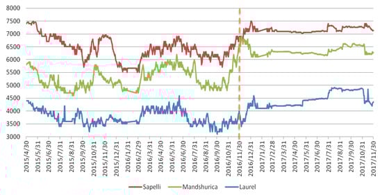
Figure 1.
The price series of three species of hardwood lumber imported by China between 30 April 2015 and 30 November 2017 (unit: CNY/m3).

Table 1.
Chow test results.
2.2. Methodology
All price series were converted to natural logarithms to reduce possible heteroscedasticity [24,33]. Two logarithmic price pairs were formed: Sapelli/Mandshurica and Mandshurica/Laurel.
2.2.1. The Linear Co-Integration Model
Linear co-integration has been widely used to explore relationships among price variables. The Johansen and Engle–Granger two-step approaches are the major methods employed. The integration order of price series data is first derived using the Dickey–Fuller GLS (DF-GLS) test or the Kwiatkowski–Phillips–Schmidt–Shin (KPSS) test. The null hypothesis of the DF-GLS test is that the variable is nonstationary; the KPSS test assumes that the variable is stationary. If all price series have the same unit roots, Johansen co-integration analysis is appropriate. Johansen (1988), Johansen and Juselius (1990) showed that two-dimensional vector autoregression could be written in the following “error correction” form [37,38]:
where = () is the pair of prices and , N is the lag number, and is the two-dimensional error vector with a zero mean ( is the variance-covariance matrix). Two quantitative relationships hold among the coefficients (): and , where I is an identity matrix and i is the lag order. The Johansen trace and maximum eigenvalue statistics are used to determine the number of co-integrations between the two price variables. Co-integration of each price pair was tested over both subperiods. The number of lags in each vector autoregressive model (VAR) was determined by reference to the lowest Akaike information criterion and Bayesian information criterion (AIC and BIC, respectively).
Depending on the results of the Johansen test, the Engel–Granger two-step method can be employed to explore the co-integration relationship. The method focuses on the time series properties of residuals under long-term equilibrium [39]. The Engle–Granger two-step formulae are as follows:
where are coefficients, is the error term, is the estimated residuals, is the first difference, is a white noise disturbance term, and P is the lag number. The method involves two steps. The first step estimates the long-term relationship of Equation (3) in terms of the price variables. It is essential to define the direction of information flow between long-term equilibrium prices; the Granger causality test may be helpful to this end [24]. We constructed two long-term relationships (Sapelli/Mandshurica and Mandshurica/Laurel). In the second step, the estimated residuals are used to perform a unit root test [39]. The lag number must be selected to ensure the absence of any serial correlation in the regression residuals ; the Ljung-Box Q test, and the AIC and BIC are helpful. Once the null hypothesis of = 0 is rejected, the residual series derived from the long-term equilibrium is deemed to be stationary, thus demonstrating that the two price variables are co-integrated [40].
2.2.2. The Threshold Co-Integration Model
The linear co-integration model assumes the symmetry of price transmission to capture symmetric price adjustment. However, to obtain empirical evidence of APT, Enders and Siklos [41] developed a two-step approach for examining threshold co-integration based on the approach of Engle and Granger [39]. It was suggested that the new, nonlinear co-integration model can be used as an alternative method to capture sharp asymmetric movements in a series of estimated residuals. The threshold co-integration model has advantages over other econometric methods for APT, including partial adjustment model [42,43], deterministic regime switching model [44,45], and so on. First, it can apply the standardized cointegrating Dickey–Fuller technique to survey asymmetric adjustment to the long run equilibrium [10]. Second, it can be used to investigate the magnitude and speed of price transmission [31].
Estimation proceeds as follows. First, using the ordinary least-squares method, the long-term equilibrium relationships between price series are derived using Equation (3). Second, the estimated residuals and forming indicators are used to create a threshold autoregression (TAR) model and a momentum threshold autoregression (MTAR) model. The principal equation is Equation (5); Equations (6a) and (6b) yield the indicator variables:
where represents the Heaviside indicator, P is the lag number, and are coefficients, and is the threshold value. The lag P deals with serially correlated residuals, and is selected using the AIC, BIC, or Ljung-Box Q test. Equations (5) and (6a) represent the TAR model ( = 0), where the indicator variable depends on the previous period residual . The adjustment is modeled using if is above the threshold; is used if is below the threshold. Similarly, Equations (5) and (6b) represent the MTAR model ( = 0); the previous period change now becomes the key adjustment variable, similar to above. In this manner, the TAR captures potential asymmetric deep movements in the residuals; the MTAR model considers steep variations in the residuals. Both methods can be used to capture the potential APT. However, as the MTAR uses the first-order differences of the previous-period estimated residuals as indicator variables, it optimally considers sharper asymmetric price changes [39,41].
If the threshold value is zero, some bias may be introduced. Chan [46] proposed an improved method for threshold selection, which includes three steps as follows. The first step involves placing the possible residuals of the TAR model or the values of the MTAR model in ascending order. Next, after excluding 15% of both the largest and smallest values, the best threshold values are determined using the remaining 70% of the values. In the final step, by calculating and comparing the sum-of-squares errors of all potential thresholds, the threshold with the minimum sum serves as a consistent estimate of the threshold value . Models with consistent thresholds are termed consistent TAR (CTAR) or consistent MTAR (CMTAR) models, which possess the similar features of the TAR and MTAR models described above.
Given the estimated threshold values, consistent models (CTAR—Equation (6a) with an estimated , and CMTAR—Equation (6b) with an estimated ) were employed to evaluate each price pair. Furthermore, two F-statistics were used to test the features of the two models. The rejection of the null hypothesis (no co-integration) indicates that co-integration relationships exist between the two price series, as revealed by the unique critical values [41]. Another standard F-test was employed to examine the null hypothesis of symmetric adjustment. A negative residual deepness (i.e., ≤ ) suggests that increases are likely to persist; decreases tend to revert faster toward the equilibrium. According to Enders and Granger [47], the model with the lowest AIC and BIC will be optimal for further analysis.
The convergence rates of price deviations to the long-term equilibrium in the threshold regression model can be estimated as follows [25]:
where n denotes the number of days, q is the proportion of price adjustment, and the absolute value of represents the speed of price adjustment to the equilibrium.
2.2.3. Threshold Error Correction Model
To incorporate the effects of asymmetry into the models of price transmission, a TECM was initially developed and then extended by many authors [47,48,49]. We decompose the error correction terms into positive and negative components to focus on whether positive and negative price differences exert asymmetric effects on short-term dynamic price behaviors. The error correction models are built based on long-term correction of asymmetric relationships, as follows:
where are coefficients and constants, is an error correction term, t is the time, and j is the lag order. The maximum lag J is chosen using the AIC statistic and the Ljung-Box Q test; the latter test deals with serial correlation. The error correction term is split into positive and negative components (+ and −); and are both defined using the best-fit model. After estimating short-term asymmetric adjustments by threshold, two F-tests are performed: one to explore the weak exogeneity of price variables () and the other to examine asymmetry status ().
3. Results
3.1. Linear Co-Integration Analysis
The KPSS and DF-GLS indicated that the price series was non-stationary; all prices exhibited a single order of integration in both subperiods (Table 2). When the Johansen approach was used to analyze the first and second subperiods (Table 3), the appropriate lag numbers were 2 and 4, respectively. For both price pairs, the Johansen trace and maximum eigenvalue test results rejected the null hypothesis (no co-integration); both price pairs exhibited single co-integration relationships in both subperiods. As shown in Table 4, in each subperiod, Sapelli was the Granger cause of Mandshurica, and Mandshurica was the Granger cause of Laurel. Thus, Sapelli is the independent variable for the price pair Sapelli/Mandshurica, and Mandshurica is the independent variable for the price pair Mandshurica/Laurel (Equation (3)). The Engle–Granger estimates yielded by Equation (4) are shown in Table 5 and Table 6. The null hypothesis of = 0 is rejected at the 10% significance level (at least) for each price pair over the entire period. The Engle–Granger approach clearly shows that both price pairs are co-integrated in both subperiods.
Table 2.
Unit root test results.
Table 3.
Results of Johansen co-integration test of pairwise logarithmic prices.
Table 4.
Causality test results.
Table 5.
Results of the Engle–Granger and threshold cointegration model for the first subperiod.
Table 6.
Results of the Engle–Granger and threshold co-integration model for the second subperiod.
3.2. Threshold Co-Integration Analysis
The threshold co-integrations of the two price pairs in both subperiods, as revealed by the CTAR and CMTAR models, are shown in Table 5 and Table 6. All estimated thresholds were near zero; there was no “subjective setting” bias. The Ljung-Box Q tests were used to check the autocorrelation of the residuals [41]. The Ljung-Box Q statistics showed that none of the models had the problem of serial correlation at least in a lag of 8. AIC and BIC were common criteria for model selection. After initial imposition of a maximum lag of 8, the AIC and BIC statistics revealed that lags of 4 and 5 in the first and second subperiods (respectively) are sufficient. Given the AIC and BIC statistics, the CMTAR model was selected as optimal to reveal the asymmetry of steep price movements irrespective of price pair and subperiod. The following analysis is based on this model. The point estimates of the ρs have signs indicating convergence in the first subperiod (Table 5). The values are not significant for either price pair, but the values differ significantly from zero at the 1% level. Thus, positive discrepancies converged slowly toward the long-term equilibrium; negative discrepancies exhibited relatively rapid convergence. The estimated Φ-statistics are 8.537 (Sapelli/Mandshurica) and 13.099 (Mandshurica/Laurel); the null hypothesis (no co-integration of either price pair) can thus be rejected at the 1% significance level. Furthermore, the estimated F-statistics are 10.411 (Sapelli/Mandshurica) and 14.451 (Mandshurica/Laurel), allowing for the rejection of the null hypothesis (symmetric adjustment of both price pairs) at the 1% significance level. The price transmission process is asymmetric in the first subperiod for both price pairs. In the second subperiod, all point estimates of and are negative, and lie remotely from the zero (Table 6). is much smaller than for each price pair. Thus, the convergence speed of a positive deviation from the long-term equilibrium is significantly slower than that of a negative deviation. The null hypothesis (no co-integration) is rejected by the Φ-statistics (6.900 for the Sapelli/Mandshurica price pair and 9.325 for the Mandshurica/Laurel price pair); both exceed the critical value at the 5% significance level. The null hypothesis (F-test symmetry) is rejected at the 10% level for each price pair. Therefore, price adjustment asymmetry was evident for both price pairs in the second subperiod. For the Sapelli/Mandshurica price pair in the first subperiod, only the point estimates of negative deviations were significant, with a statistic of −0.0869. Thus, negative deviation (< −0.0039) from the long-term equilibrium, caused by an increase in the price of Sapelli or a decline in the price of Mandshurica, could disappear at a rate of 8.69% per day. If the proportion of a disequilibrium to be corrected is taken to be 90%, then, for = 0.0869, the number of days taken to correct 90% of the disequilibrium will be: . It thus requires less than a month to eliminate 90% of the negative disequilibrium. Similarly, for the Mandshurica/Laurel price pair in the first subperiod, about one-third of a month is needed to correct 90% of the negative change. In the second subperiod, for the Sapelli/Mandshurica price pair, the point estimates of positive and negative deviation are significant at −0.0342 and −0.0991, respectively. Thus, the positive deviation (≥ −0.0028) from the long-term equilibrium, caused by a fall in the Sapelli price or rise in the Mandshurica price, could disappear at a rate of 3.42% per day. Similarly, the negative deviation (< −0.0028) could disappear at a rate of 9.91% per day. It would thus require over two months to eliminate 90% of the positive discrepancy, but approximately two-thirds of a month to correct 90% of the negative discrepancy. For the Mandshurica/Laurel price pair in the second subperiod, disappearance of 90% of the positive disequilibrium would require more than 2.5 months; the negative disequilibrium would be corrected in less than one month.
3.3. Threshold Error Correction Analysis
In terms of short-term APT, the estimated TECMs given by Equations (8) and (9) are shown in Table 7 and Table 8, respectively. The Ljung-Box Q tests rejected the autocorrelation of the residuals at least in a lag of 8, and the AIC and BIC statistics indicated that a lag of 5 for each model was appropriate. The weak exogeneity indicated that the null hypothesis () cannot be rejected in terms of the price of the higher-quality lumber of each price pair, except for Sapelli of the Sapelli/Mandshurica pair in the second subperiod at the significance level of 1%. However, the coefficient in the Sapelli equation for Sapelli/Mandshurica is significantly larger than zero, and is essentially zero. Thus, the prices of the higher-quality lumber of each price pair evolve independently. By comparison, the weak exogeneity tests reject the null hypothesis for the lower-quality lumber of each price pair at the 5% significance level (at least). Thus, the prices of both lower-quality lumbers tend to counter the price disequilibrium. The F-statistics of the null hypothesis verify that Mandshurica of the Sapelli/Mandshurica price pair and Laurel of the Mandshurica/Laurel price pair exhibit short-term APT. In the first subperiod, for the Sapelli/Mandshurica price pair, the coefficients of the threshold error correction terms in the Sapelli equation ( and ) are not significant, implying that the price of Sapelli may have evolved independently from that of Mandshurica in the short term (Table 7). Only the coefficient of the negative error correction term of the Mandshurica equation () is significant, being −0.0729, suggesting that 7.29% of the negative price differential can be eliminated in one day, whereas the Mandshurica price does not respond to any positive price differential. A similar result is obtained for the Mandshurica/Laurel price pair. The price of Mandshurica may fluctuate independently; the negative price differential of Laurel can be adjusted by 24.01% per day, but little adjustment of the positive price differential is evident. In the second subperiod, for the price pair Sapelli/Mandshurica, Sapelli exhibited relatively autonomous price variation. Mandshurica does not react to positive deviation; the negative deviation in Mandshurica price can disappear at a rate of 8.96% per day (Table 8). Similarly, the price change of Mandshurica is undisturbed by that of Laurel in the Mandshurica/Laurel price pair. However, the Laurel equation shows that the daily adjustment speed (7.99%) of a negative change from the equilibrium is more than twice that of a positive change (2.99%).
Table 7.
Results of the threshold error correction model for the first subperiod.
Table 8.
Results of the threshold error correction model for the second subperiod.
4. Discussion
Our empirical results show that APT is evident in China’s market of imported hardwood lumber in the whole period. Whether in the first or second subperiod, the price series present positive asymmetric price transmission in the long and short term. This is, the negative price differential is adjusted by a faster convergence speed than the positive one. This is consistent with the conclusions from the majority of previous studies on spatial APT [13,34]. APT reflects a redistribution of welfare compared to the symmetrical situation, modifying the timing and/or magnitude of changes associated with price adjustments [10]. Hardwood lumber exporters respond more rapidly to negative price deviations than to positive price deviations in the Chinese market. These exporters can better take advantage of the price increases that are unavailable under symmetrical conditions; on the other hand, the hardwood lumber importers seem less responsive or lacking the ability to respond to the price reductions created by APT.
In both the long-and short-term, we find that positive differential in each price pair converges slowly in the first subperiod, while relatively fast in the second subperiod. This indicates that the hardwood lumber exporters are likely to benefit more from an increase of price in the former subperiod than in the latter. The main reason could be that the degrees of the CCLB policy intervention between both subperiods are different. Harvesting from natural forests in China fell sharply over the first subperiod, but less so in the second subperiod. The amount of logging from natural forests in China decreased by 3.56 million m3 from 2015 to 2016, while only dropped by 0.45 million m3 from 2016 to 2017 [4]. Exporters’ expectations of price rises would thus be stronger in the first subperiod than in the second one. Thus, positive price discrepancies tended to be more persistent in the former subperiod than in the latter.
5. Conclusions
We disclose that APT was evident in Chinese imported hardwood lumber market when the CCLB was implemented. By examining the Shapelli/Mandshurica and Mandshurica/Laurel price pairs, we detect a structural break at the end of the second CCLB phase, which prompts us to divide the study period into two subperiods. The break reflects the different degree of impact of different CCLB implementation phases. The CMTAR model best-fitted the price series of both subperiods, suggesting that price adjustment may be steep when asymmetry is present. The empirical results from both subperiods show that the import prices of both hardwood lumber pairs were co-integrated in a long-term relationship, and that both short-and long-term asymmetric price adjustments were evident. In the long term, the convergence rates of positive price discrepancies to the equilibrium were slower than those of negative price discrepancies. In the short term, for each pair, the price of higher-quality lumber was minimally affected by the price of lower-quality lumber, but the price of the latter type of lumber tends to follow the price of the former type. Positively asymmetric spatial price transmission in the imported hardwood lumber market of China was uncovered; interactions among price pairs were evident after the forest conservation policy was introduced.
The APT identified herein emphasizes that the hardwood lumber market is inefficient. More effective trade policies would be helpful in the CCLB era to correct for the asymmetries. It may be an effective way for China to reduce import dependence on a few countries by diversifying import sources of hardwood lumber. Furthermore, it is suggested that timber import channels should be unified by industry associations. This aims at increasing the bargaining power of China’s importers in trade negotiations. However, APT allows both importers and, to a lesser extent, foreign suppliers to strategize with respect to their responses to future price fluctuations. Various threshold co-integration models can be used to examine the markets for logs, pulpwood, and other major forest products. Such efforts would improve knowledge on the price transmission characteristics of forest products, especially in the international context.
Author Contributions
Conceptualization, Z.Y.; methodology, Z.Y., L.Y.; writing—original draft preparation, L.Y.; validation, L.Y., Z.Y.; formal analysis, L.Y.; investigation, L.Y., F.W.; data curation, F.W.; writing—review and editing, Z.Y., J.G.; supervision, J.G. All authors have read and agreed to the published version of the manuscript.
Funding
This research was financially supported by the Fundamental Research Funds for the Central Universities (Grant No. 2018RW15, Grant No. JGZKPY009, Grant No. 2019YC20), the Ministry of Education Humanities and Social Sciences Project (Grant No. 18YJA790096), the National Natural Science Foundation of China (Grant No. 71350017), and China Scholarship Council Fund. However, opinions expressed here do not reflect the funding agencies’ view.
Conflicts of Interest
The authors declare no conflict of interest.
References
- State Forestry Administration in China. The eighth national forest resources inventory. For. Resour. Manag. 2014, 1, 1–2, (Translated title into English). [Google Scholar]
- State Forestry Administration in China. The Report of Forestry Development in China, 1st ed.; China Forestry Publishing House: Beijing, China, 2015; (Translated title into English).
- United Nations Comtrade. Available online: http://comtrade.un.org/db/ (accessed on 10 July 2019).
- Economy Prediction System. Available online: http://www.epsnet.com.cn/index.html (accessed on 10 July 2019).
- Chen, X.; Chinese Society of Forestry; Ju, Q.; Lin, K. Current situation, problems and countermeasures of plantation development in China. World For. Res. 2014, 27, 54–59, (Translated title into English). [Google Scholar] [CrossRef]
- Xue, W. Problems and countermeasures in the quality of plantation in China. Mod. Hortic. 2015, 5, 100–101, (Translated title into English). [Google Scholar] [CrossRef]
- Wang, H.; Guo, J. Status quo of artificial forest in China and its near-natural management. Mod. Agric. Sci. 2008, 15, 124–125, (Translated title into English). [Google Scholar]
- Ghoshray, A. An examination of the relationship between U.S. and Canadian durum wheat prices. Can. J. Agric. Econ. Rev. Can. Agroecon. 2007, 55, 49–62. [Google Scholar] [CrossRef]
- Blinder, A.S.; Canetti, E.R.; Lebow, D.E.; Rudd, J.B. Asking about Prices: A New Approach to Understanding Price Stickiness; Russel Sage Foundation: New York, NY, USA, 1998. [Google Scholar]
- Meyer, J.; Cramon-Taubadel, S. Asymmetric price transmission: A survey. J. Agric. Econ. 2004, 55, 581–611. [Google Scholar] [CrossRef]
- Simioni, M.; Gonzales, F.; Guillotreau, P.; Le Grel, L. Detecting asymmetric price transmission with consistent threshold along the fish supply chain. Can. J. Agric. Econ. Rev. Can. Agroecon. 2013, 61, 37–60. [Google Scholar] [CrossRef]
- Forker, K.O.D. Asymmetry in farm-retail price transmission for major dairy products. Am. J. Agric. Econ. 1987, 69, 285–292. [Google Scholar] [CrossRef]
- Frey, G.; Manera, M. Econometric models of asymmetric price transmission. J. Econ. Surv. 2007, 21, 349–415. [Google Scholar] [CrossRef]
- Peltzman, S. Prices rise faster than they fall. J. Political Econ. 2000, 108, 466–502. [Google Scholar] [CrossRef]
- Shrinivas, A.; Gomez, M.I. Price transmission, asymmetric adjustment and threshold effects in the cotton supply chain: A case study for Vidarbha, India. Agric. Econ. 2016, 47, 435–444. [Google Scholar] [CrossRef]
- Ahn, B.; Lee, H. Vertical price transmission of perishable products: The case of fresh fruits in the Western United States. J. Agric. Resour. Econ. 2015, 40, 405–424. [Google Scholar]
- Durborow, S.L.; Chung, C.; Kim, S. Implications of the 2006 E. coli outbreak on spatial price transmission in the US fresh spinach market. Agribusiness 2017, 33, 475–492. [Google Scholar] [CrossRef]
- Chavas, J.P.; Mehta, A. Price dynamics in a vertical sector: The case of butter. Agric. Econ. 2004, 86, 1078–1093. [Google Scholar] [CrossRef]
- Abdulai, A. Using threshold cointegration to estimate asymmetric price transmission in the Swiss pork market. Appl. Econ. 2002, 34, 679–687. [Google Scholar] [CrossRef]
- Ankamah-Yeboah, I.; Bronnmann, J. Asymmetries in import-retail cost pass-through: Analysis of the seafood value chain in Germany. Aquac. Econ. Manag. 2017, 21, 71–87. [Google Scholar] [CrossRef]
- Jong-Yeol, Y.; Brown, S. An asymmetric price transmission analysis in the U.S. pork market using threshold co-integration analysis. J. Rural Dev. 2018, 41, 41–66. [Google Scholar]
- Alam, M.J.; McKenzie, A.M.; Begum, I.A.; Buysse, J.; Wailes, E.J.; Van Huylenbroeck, G. Asymmetry price transmission in the deregulated rice markets in Bangladesh: Asymmetric error correction model. Agribusiness 2016, 32, 498–511. [Google Scholar] [CrossRef]
- Abdulai, A. Spatial price transmission and asymmetry in the Ghanaian maize market. J. Dev. Econ. 2000, 63, 327–349. [Google Scholar] [CrossRef]
- Ganneval, S. Spatial price transmission on agricultural commodity markets under different volatility regimes. Econ. Model. 2016, 52, 173–185. [Google Scholar] [CrossRef]
- Ghoshray, A. Agricultural economics society prize essay asymmetric price adjustment and the world wheat market. J. Agric. Econ. 2002, 53, 299–317. [Google Scholar] [CrossRef]
- Fiamohe, R.; Seck, P.A.; Alia, D.Y.; Diagne, A. Price transmission analysis using threshold models: An application to local rice markets in Benin and Mali. Food Secur. 2013, 5, 427–438. [Google Scholar] [CrossRef]
- Jamora, N.; von Cramon-Taubadel, S. Transaction cost thresholds in international rice markets. J. Agric. Econ. 2016, 67, 292–307. [Google Scholar] [CrossRef]
- Usman, M.A.; Haile, M.G. Producer to retailer price transmission in cereal markets of Ethiopia. Food Secur. 2017, 9, 815–829. [Google Scholar] [CrossRef]
- Svanidze, M.; Goetz, L.; Djuric, I.; Glauben, T. Food security and the functioning of wheat markets in Eurasia: A comparative price transmission analysis for the countries of Central Asia and the South Caucasus. Food Secur. 2019, 11, 733–752. [Google Scholar] [CrossRef]
- Alemu, Z.G.; Ogundeji, A.A. Price transmission in the South African food market. Agrekon 2010, 49, 433–445. [Google Scholar] [CrossRef]
- Koutroumanidis, T.; Zafeiriou, E.; Arabatzis, G. Asymmetry in price transmission between the producer and the consumer prices in the wood sector and the role of imports: The case of Greece. For. Policy Econ. 2009, 11, 56–64. [Google Scholar] [CrossRef]
- Ahn, B.; Lee, H. Asymmetric transmission between factory and wholesale prices in fiberboard market in Korea. J. For. Econ. 2013, 19, 1–14. [Google Scholar] [CrossRef]
- Ning, Z.; Sun, C. Vertical price transmission in timber and lumber markets. J. For. Econ. 2014, 20, 17–32. [Google Scholar] [CrossRef]
- Sun, C. Price dynamics in the import wooden bed market of the United States. For. Policy Econ. 2011, 13, 479–487. [Google Scholar] [CrossRef]
- Guo, X.; Ran, J. Imported Timber Atlas, 2nd ed.; Shanghai Science and Technology: Shanghai, China, 2016; pp. 25–28, 175, 222. [Google Scholar]
- Perron, P. Further evidence on breaking trend functions in macroeconomic variables. J. Econom. 1997, 80, 355–385. [Google Scholar] [CrossRef]
- Johansen, S. Statistical analysis of cointegration vectors. J. Econ. Dyn. Control 1988, 12, 231–254. [Google Scholar] [CrossRef]
- Johansen, S.; Juselius, K. Maximum likelihood estimation and inference on cointegration—With applications to the demand for money. Oxf. Bull. Econ. Stat. 1990, 52, 169–210. [Google Scholar] [CrossRef]
- Engle, R.F.; Granger, C.W.J. Cointegration and error correction: Representation, estimation, and testing. Econometrica 1987, 55, 251–276. [Google Scholar] [CrossRef]
- Enders, W. Applied Econometric Time Series, 3rd ed.; John Wiley & Sons: Hoboken, NJ, USA, 2010. [Google Scholar]
- Enders, W.; Siklos, P.L. Cointegration and threshold adjustment. J. Bus. Econ. Stat. 2001, 19, 166–176. [Google Scholar] [CrossRef]
- Bacon, R.W. Rockets and feathers: The asymmetric speed of adjustment of UK retail gasoline prices to cost changes. Energy Econ. 1991, 13, 211–218. [Google Scholar] [CrossRef]
- Shin, D. Do product prices respond symmetrically to changes in crude oil prices? OPEC Rev. 1994, 18, 137–157. [Google Scholar] [CrossRef]
- Goodwin, B.K.; Holt, M.T. Price transmission and asymmetric adjustment in the U.S. beef sector. Am. J. Agric. Econ. 1999, 81, 630–637. [Google Scholar] [CrossRef]
- Goodwin, B.K.; Piggott, N.E. Spatial market integration in the presence of threshold effects. Am. J. Agric. Econ. 2001, 83, 302–317. [Google Scholar] [CrossRef]
- Chan, K.S. Consistency and limiting distribution of the least squares estimator of a threshold autoregressive model. Ann. Stat. 1993, 21, 520–533. [Google Scholar] [CrossRef]
- Enders, W.; Granger, C.W.J. Unit-root tests and asymmetric adjustment with an example using the term structure of interest rates. J. Bus. Econ. Stat. 1998, 16, 304–311. [Google Scholar] [CrossRef]
- Balke, N.S.; Fomby, T.B. Threshold cointegration. Int. Econ. Rev. 1997, 38, 627–645. [Google Scholar] [CrossRef]
- Granger, C.W.J.; Lee, T.H. Investigation of production, sales and inventory relationships using multicointegration and non-symmetric error correction models. J. Appl. Econom. 1989, 4, S145–S159. [Google Scholar] [CrossRef]
© 2020 by the authors. Licensee MDPI, Basel, Switzerland. This article is an open access article distributed under the terms and conditions of the Creative Commons Attribution (CC BY) license (http://creativecommons.org/licenses/by/4.0/).