Detecting Dead Standing Eucalypt Trees from Voxelised Full-Waveform Lidar Using Multi-Scale 3D-Windows for Tackling Height and Size Variations

 ,
,  ,
, 
Abstract
1. Introduction
2. Materials and Methods
2.1. Materials
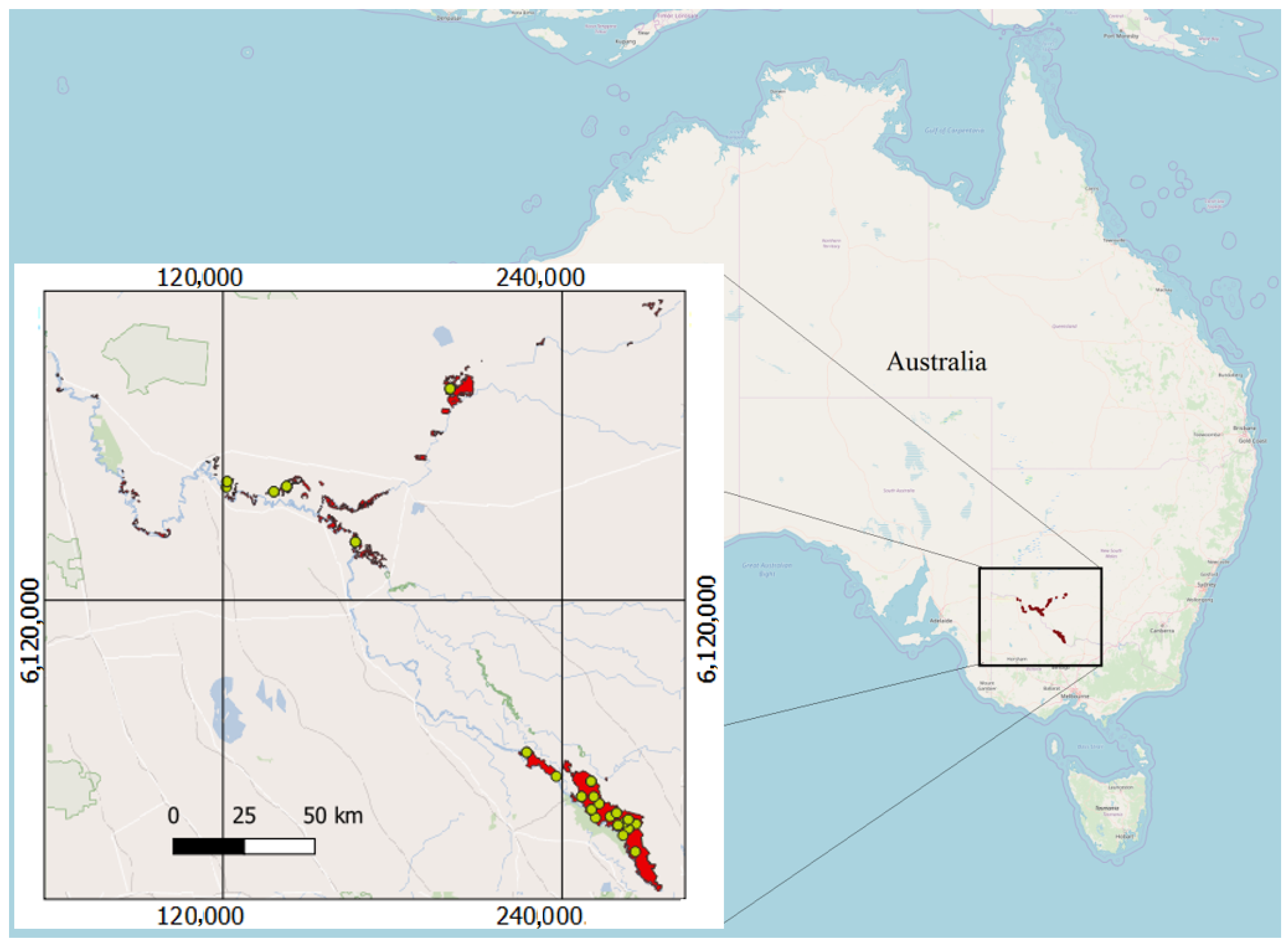
2.1.1. Study Area
2.1.2. Acquired Full-Waveform LiDAR
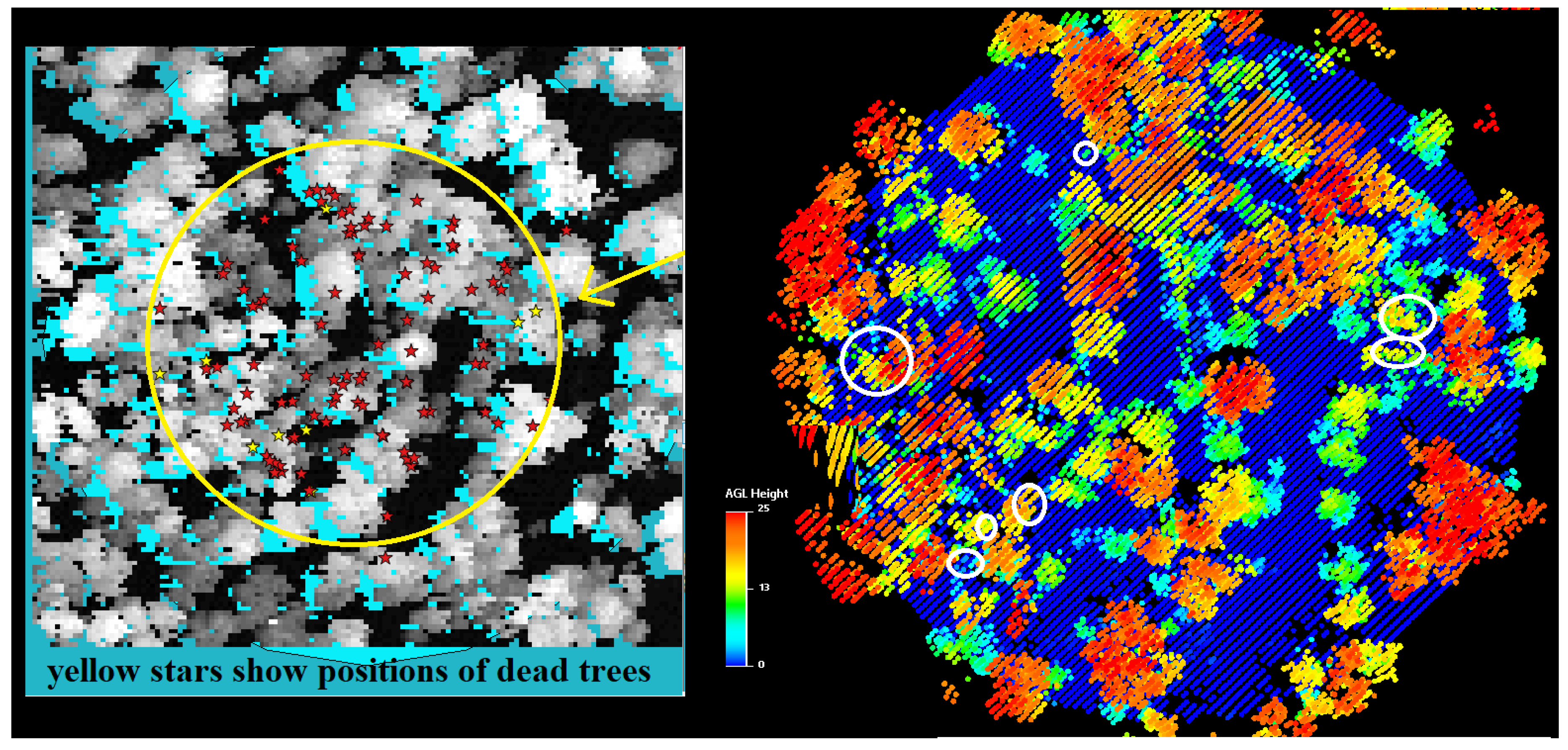
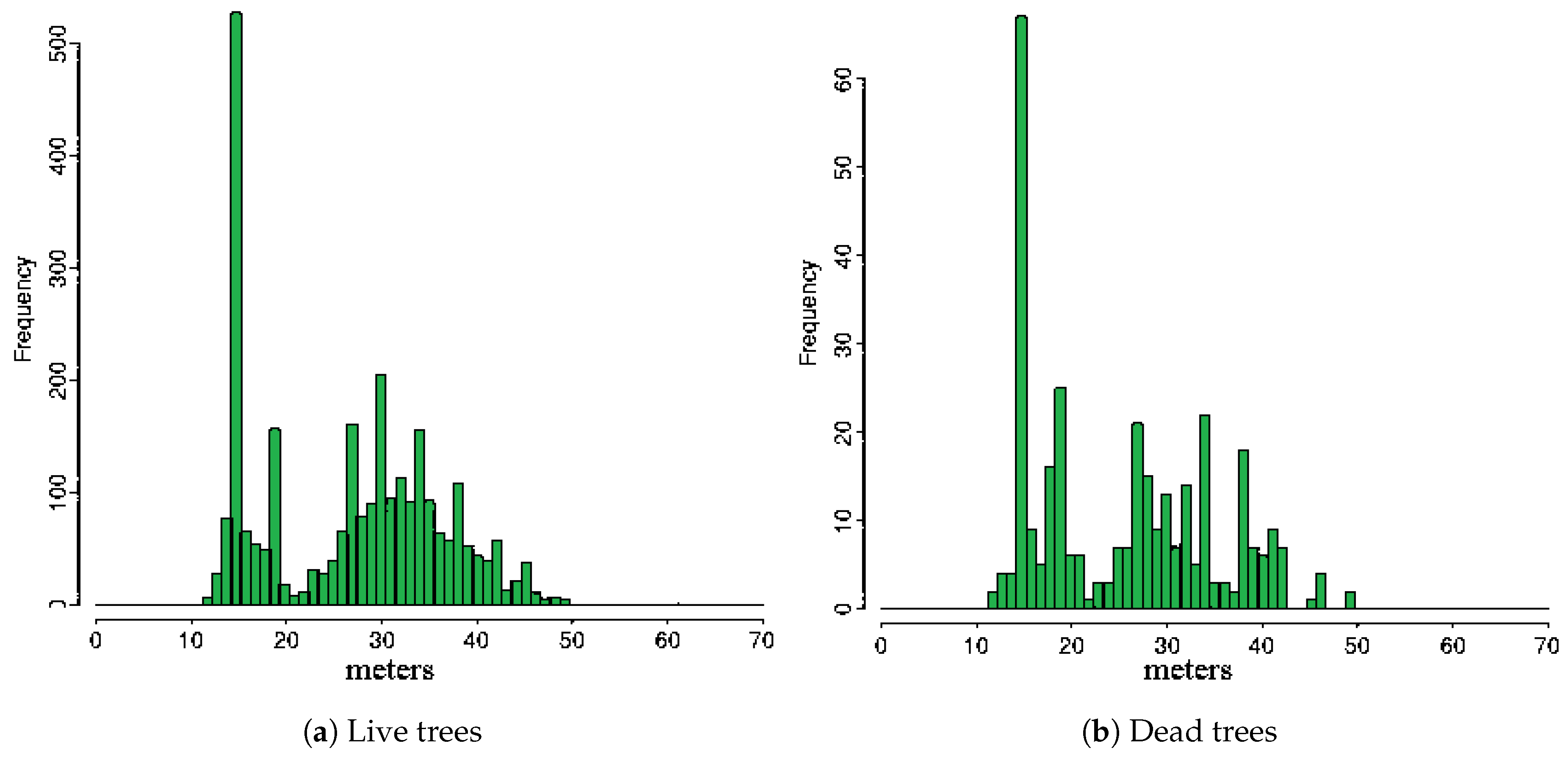
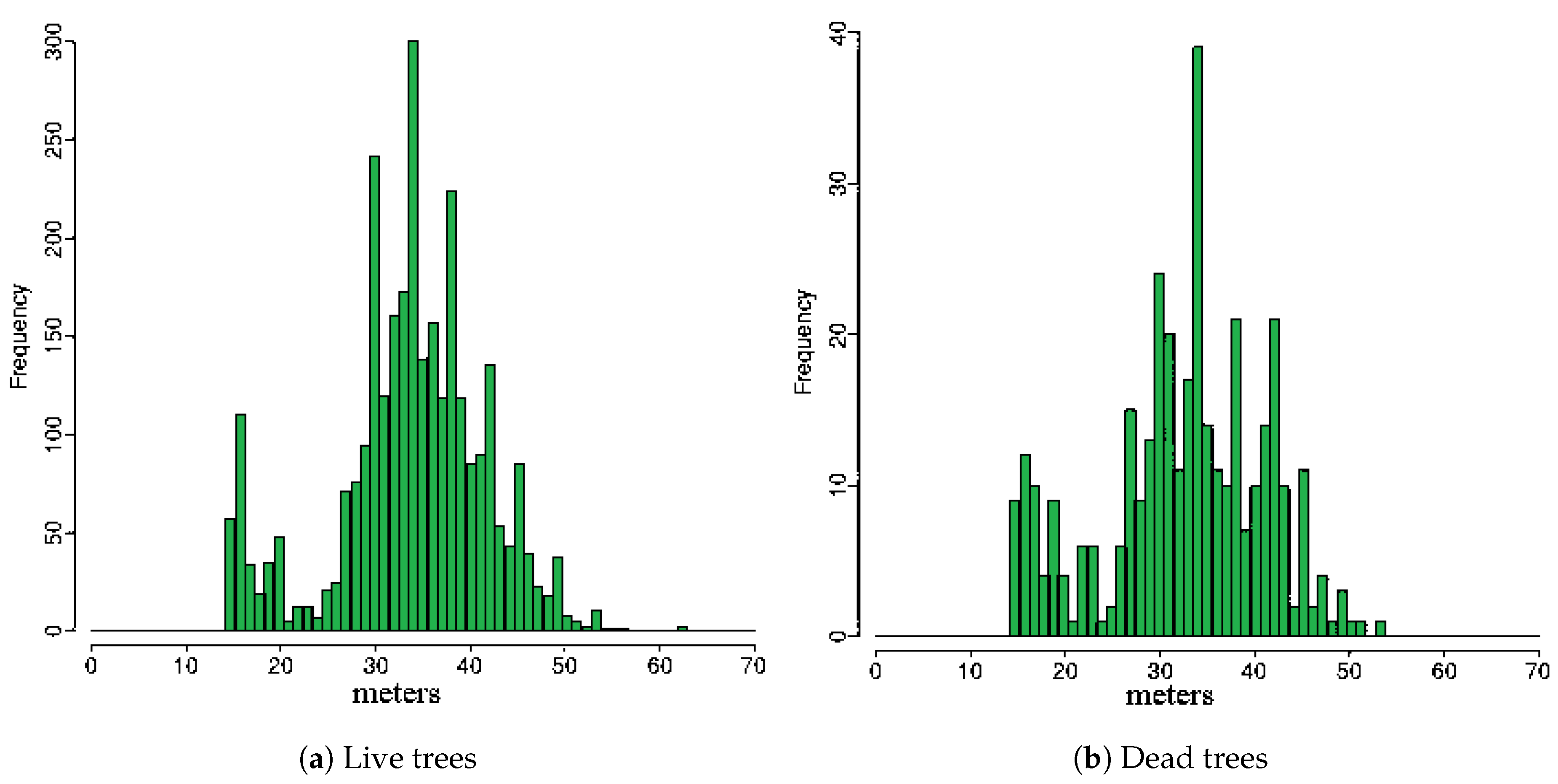
2.1.3. Field Data
2.2. Methodology
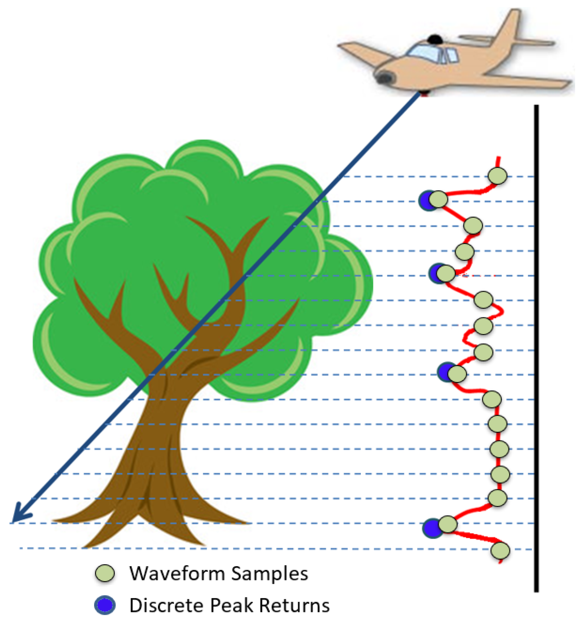
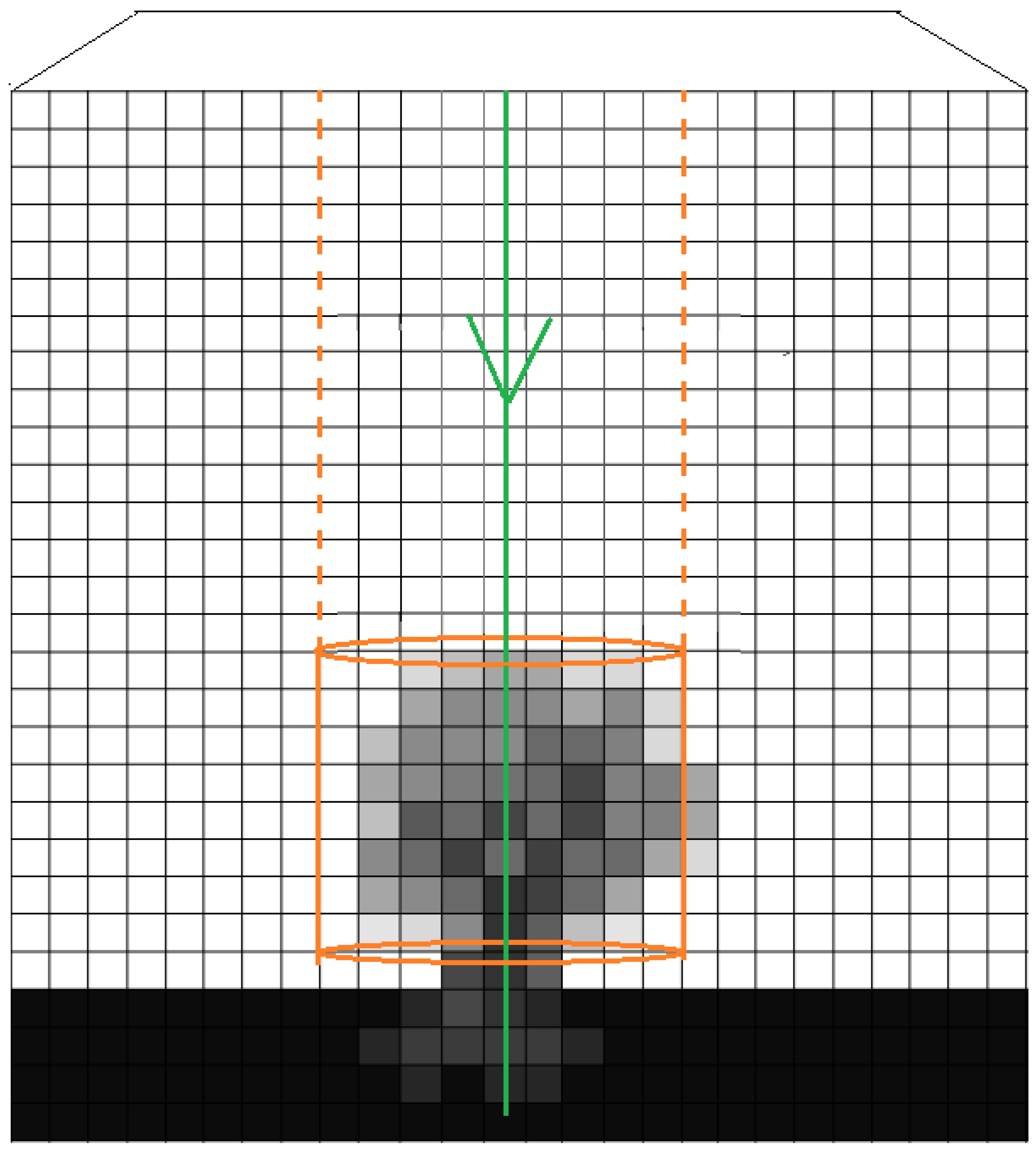
2.2.1. Voxelisation of Waveform Samples
- The space is divided into a 3D regular grid; each cube is named voxel
- Noise reduction by applying low level filtering—in other words ignore waveform sample with low intensity profile since they most probably contain noise
- Each waveform sample - whose position is calculated as explained in Section 2.1.2—is associated with the voxel that it lies inside
- Each voxel takes as value the average intensity of the waveforms that are associated with it
- The result is a discrete density volune (can be interpreted as a 3D grayscale image) with accumulated intensities of the waveforms
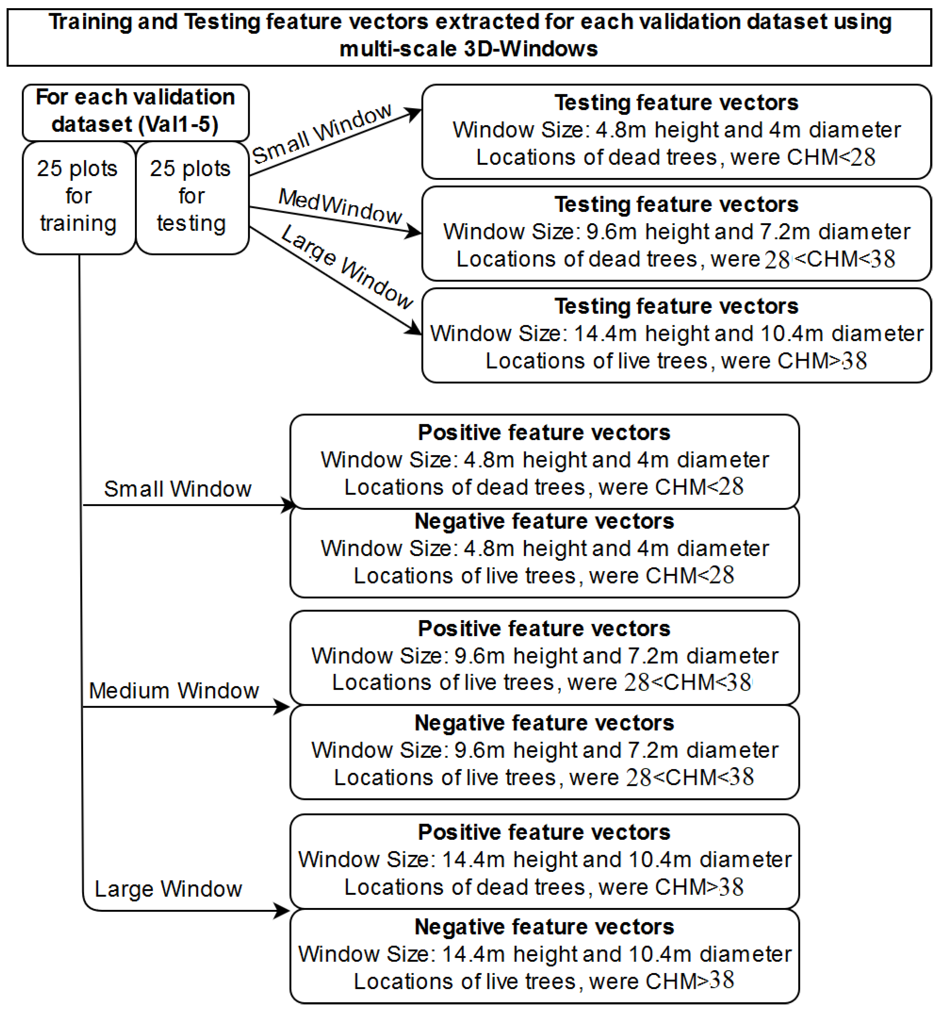
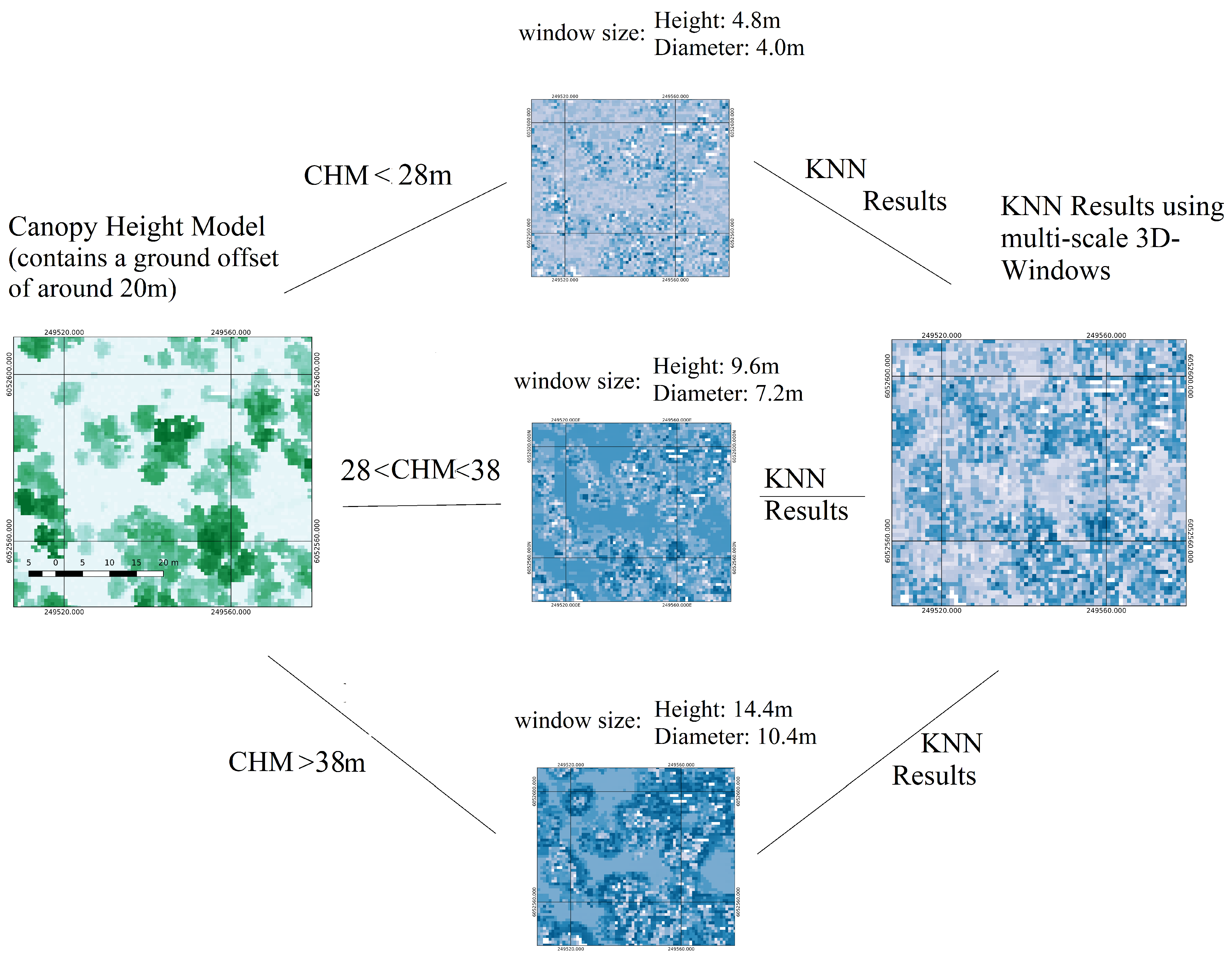
2.2.2. Extraction of Features from 3D-Windows
2.2.3. Random Forest
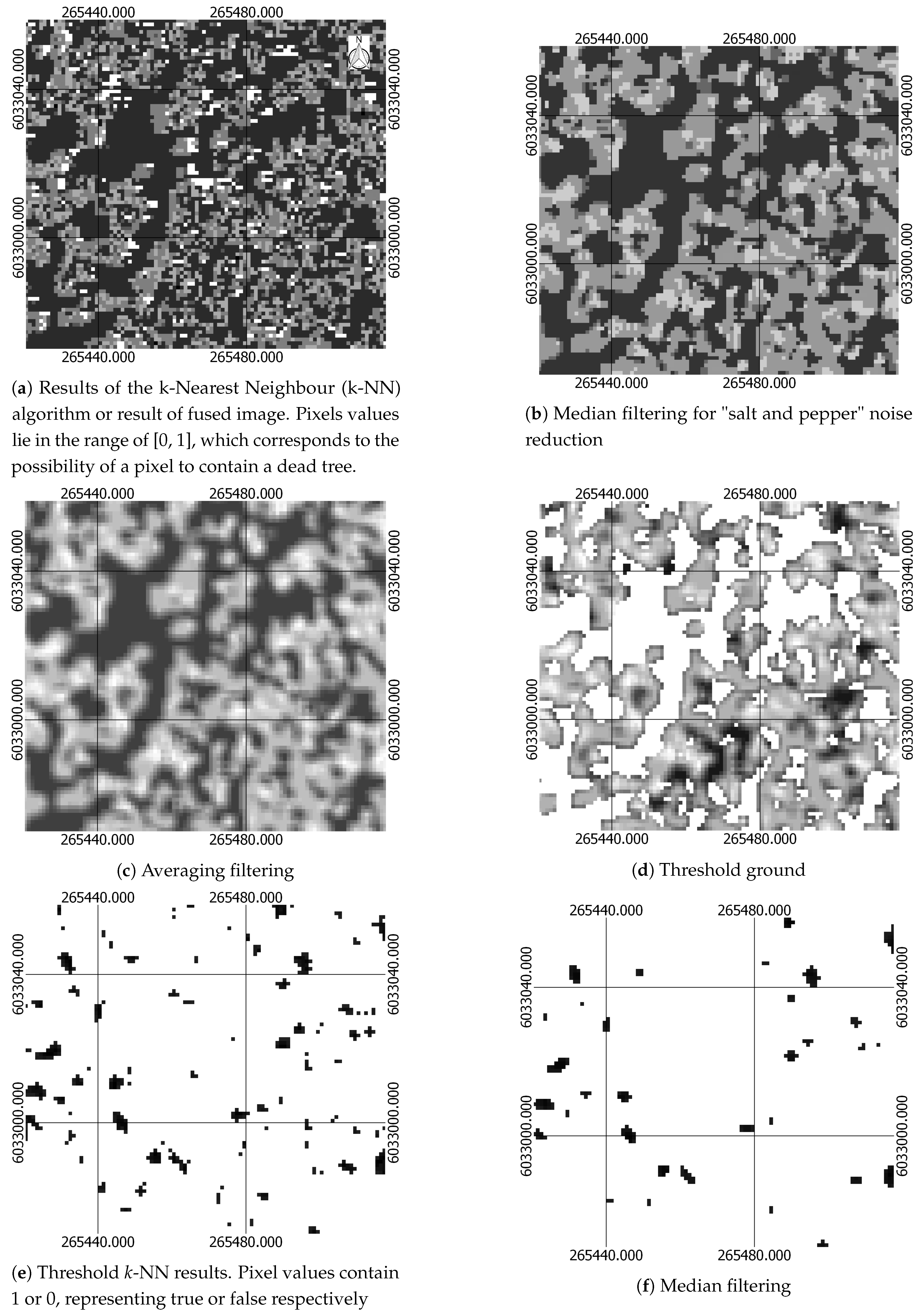
2.2.4. Weighted k-Nearest Neighbours Algorithm
2.2.5. Fusion of Probabilistic Field
2.2.6. Location detection
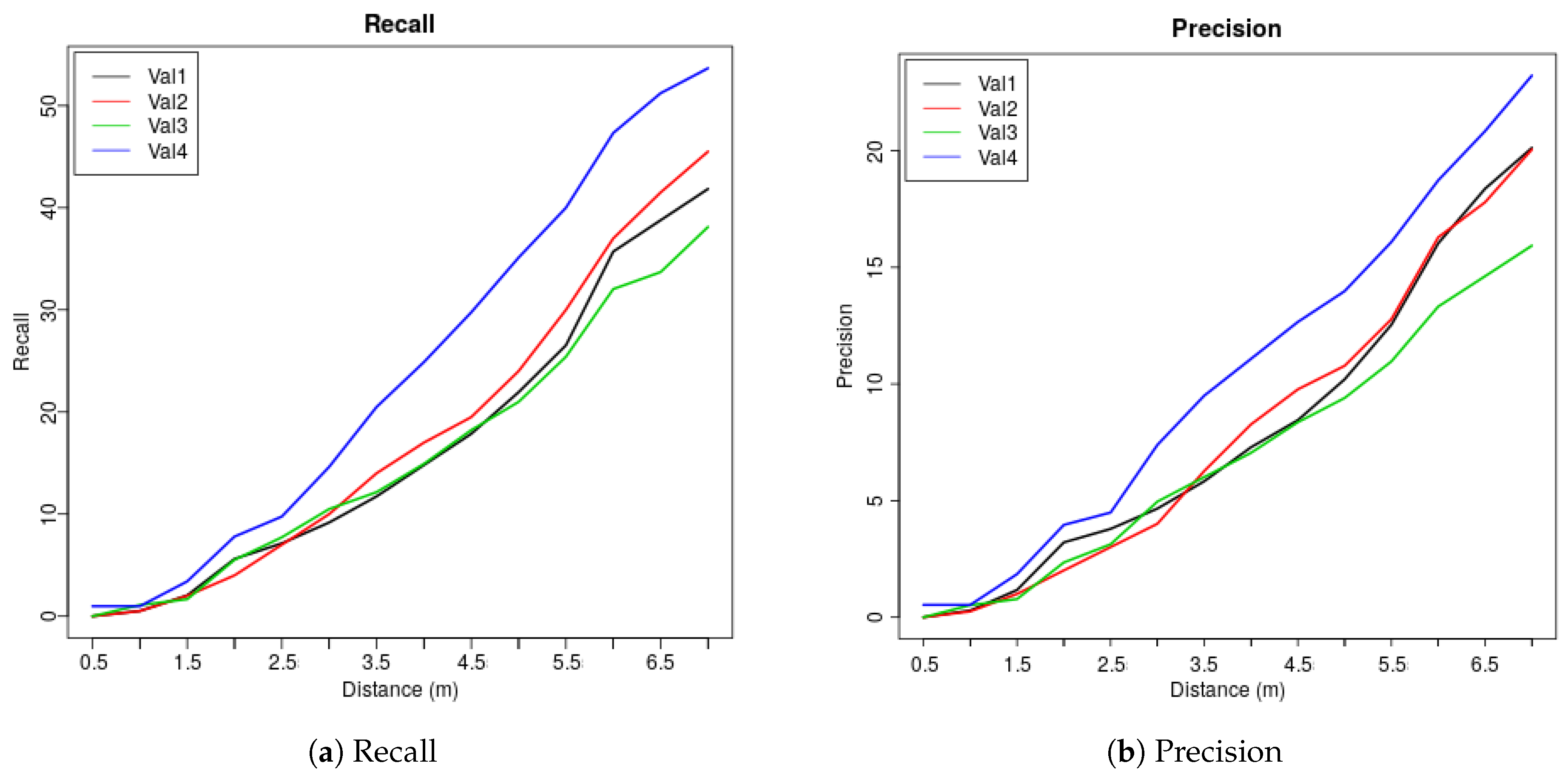
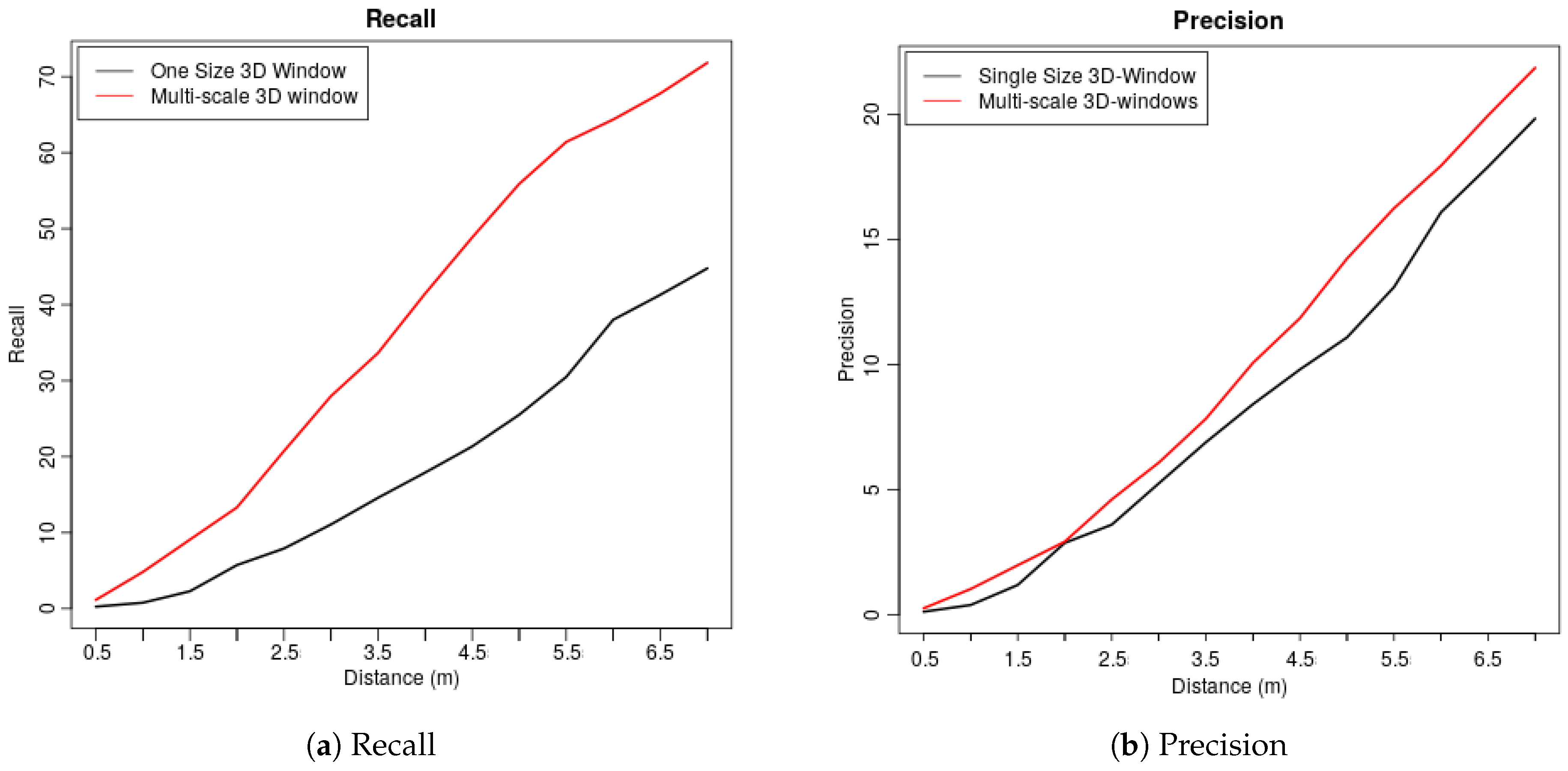
2.2.7. Cross Validation, Precision and Recall
- True Positives (): how many dead trees the system detected correctly
- False Positive (): how many locations the system wrongly labelled as dead trees
- False Negatives (): how many dead trees were not detected
- : is the number of locations that the classifier predicted that a dead tree exist
- : is the number of dead trees that existed within the field data
3. Results
4. Discussion
5. Conclusions
Author Contributions
Funding
Acknowledgments
Conflicts of Interest
Abbreviations
| CHM | Canopy Height Model |
| EU | European Union |
| FN | False Negative |
| FP | False Positive |
| H2020 | Horizon 2020 |
| k-NN | k Nearest Neighbour |
| LiDAR | Light Detection and Ranging |
| Ltd | Limited |
| NSW | New South Wells |
| TN | True Negative |
| TP | True Positive |
| SVM | Support Vector Machine |
References
- Franklin, J.F.; Shugart, H.H.; Harmon, M.E. Tree death as an ecological process. BioScience 1987, 17, 550–556. [Google Scholar] [CrossRef]
- Lindenmayer, D.B.; Cunningham, R.B.; Donnelly, C.F. Decay and Collapse of Trees with Hollows in Eastern Australian Forests: Impacts on Arboreal Marsupials. Ecol. Appl. 1997, 7, 625–641. [Google Scholar] [CrossRef]
- Zielewska-Büttner, K.; Heurich, M.; Müller, J.; Braunisch, V. Remotely Sensed Single Tree Data Enable the Determination of Habitat Thresholds for the Three-Toed Woodpecker (Picoides tridactylus). Remote Sens. 2018, 10, 1972. [Google Scholar] [CrossRef]
- Ranius, T.; Fahrig, L. Targets for maintenance of dead wood for biodiversity conservation based on extinction thresholds. Scand. J. For. Res. 2006, 21, 201–208. [Google Scholar] [CrossRef]
- Rose, C.L.; Marcot, B.G.; Mellen, T.K.; Ohmann, J.L.; Waddell, K.L.; Lindley, D.L.; Schreiber, B. Decaying wood in Pacific Northwest forests: Concepts and tools for habitat management. In Wildlife-Habitat Relationships in Oregon and Washington; Oregon State University Press: Corvallis, OR, USA, 2001; pp. 580–623. [Google Scholar]
- George, A.K.; Walker, K.F.; Lewis, M.M. Population status of eucalypt trees on the River Murray floodplain, South Australia. River Res. Appl. 2005, 21, 271–282. [Google Scholar] [CrossRef]
- Dexter, B.; Rose, H.; Davies, N. River regulation and associated forest management problems in the River Murray red gum forests. Aust. For. 1986, 49, 16–27. [Google Scholar] [CrossRef]
- Maheshwari, B.; Walker, K.; McMahon, T. Effects of regulation on the flow regime of the River Murray, Australia. Regul. Rivers Res. Manag. 1995, 10, 15–38. [Google Scholar] [CrossRef]
- Jensen, A.E.; Walker, K.F. Sustaining recovery in red gum, black box and lignum in the Murray River Valley: Clues from natural phenological cycles to guide environmental watering. Trans. R. Soc. S. Aust. 2017, 141, 209–229. [Google Scholar] [CrossRef]
- George, A.K. Eucalypt Regeneration on the Lower Murray Floodplain, South Australia. Ph.D. Thesis, University of Adelaide, Adelaide, Australia, 2004. [Google Scholar]
- Bennett, A.; Lumsden, L.; Nicholls, A. Tree hollows as a resource for wildlife in remnant woodlands: Spatial and temporal patterns across the northern plains of Victoria, Australia. Pacif. Conserv. Biol. 1994, 1, 222–235. [Google Scholar] [CrossRef]
- Gibbons, P.; Lindenmayer, D. Tree Hollows and Wildlife Conservation in Australia; CSIRO Publishing: Collingwood, Australia, 2002. [Google Scholar] [CrossRef]
- Wormington, K.; Lamb, D. Tree hollow development in wet and dry sclerophyll eucalypt forest in south-east Queensland, Australia. Austr. For. 1999, 62, 336–345. [Google Scholar] [CrossRef]
- Gibbons, P.; Lindenmayer, D.; Barry, S.C.; Tanton, M. Hollow formation in eucalypts from temperate forests in southeastern Australia. Pacif. Conserv. Biol. 2000, 6, 218. [Google Scholar] [CrossRef]
- Lindenmayer, D.B.; Wood, J.T. Long-term patterns in the decay, collapse, and abundance of trees with hollows in the mountain ash (Eucalyptus regnans) forests of Victoria, southeastern Australia. Can. J. For. Res. 2010, 40, 48–54. [Google Scholar] [CrossRef]
- Goldingay, R.L. Characteristics of tree hollows used by Australian birds and bats. Wildl. Res. 2009, 36, 394–409. [Google Scholar] [CrossRef]
- Lopes Queiroz, G.; McDermid, G.J.; Castilla, G.; Linke, J.; Rahman, M.M. Mapping Coarse Woody Debris with Random Forest Classification of Centimetric Aerial Imagery. Forests 2019, 10, 471. [Google Scholar] [CrossRef]
- Wing, B.M.; Ritchie, M.W.; Boston, K.; Cohen, W.B.; Olsen, M.J. Individual snag detection using neighborhood attribute filtered airborne lidar data. Remote Sens. Environ. 2015, 163, 165–179. [Google Scholar] [CrossRef]
- Polewski, P.; Yao, W.; Heurich, M.; Krzystek, P.; Stilla, U. Detection of fallen trees in ALS point clouds using a Normalized Cut approach trained by simulation. ISPRS J. Photogramm. Remote Sens. 2015, 105, 252–271. [Google Scholar] [CrossRef]
- Mücke, W.; Deák, B.; Schroiff, A.; Hollaus, M.; Pfeifer, N. Detection of fallen trees in forested areas using small footprint airborne laser scanning data. Can. J. Remote Sens. 2013, 139, S32–S40. [Google Scholar] [CrossRef]
- Pasher, J.; King, D.J. Mapping dead wood distribution in a temperate hardwood forest using high resolution airborne imagery. For. Ecol. Manag. 2009, 258, 1536–1548. [Google Scholar] [CrossRef]
- Yao, W.; Krzystek, P.; Heurich, M. Identifying Standing dead trees in forest areas based on 3D single tree detection from full-waveform LiDAR data. ISPRS Ann. Photogramm. Remote Sens. Spat. Inf. Sci. 2012, I-7, 359–364. [Google Scholar] [CrossRef]
- Shendryk, I.; Broich, M.; Tulbure, M.G.; McGrath, A.; Keith, D.; Alexandrov, S.V. Mapping individual tree health using full-waveform airborne laser scans and imaging spectroscopy: A case study for a floodplain eucalypt forest. Remote Sens. Environ. 2016, 187, 202–217. [Google Scholar] [CrossRef]
- Grant, M. LIDAR Processing Notes; NERC Airborne Research Facility, Plymouth Marine Laboratory; NERC-ARF: Plymouth, UK, 2008. [Google Scholar]
- ASPRS. LAS Specification: Version 1.3–R11; The American Society for Photogrammetry and Remote Sensing: Bethesda, MD, USA, 2010. [Google Scholar]
- ASPRS. LAS Specification: Version 1.4–R13; The American Society for Photogrammetry and Remote Sensing: Bethesda, MD, USA, 2013. [Google Scholar]
- Rapidlasso. PulseWaves - Full Waveform LiDAR Specification (Version 0.3 Revision 11); Rapidlasso: Gilching, Germany, 2015. [Google Scholar]
- Wanger, W.; Ullrich, A.; Ducic, V.; Maizer, T.; Studnicka, N. Gaussian decompositions and calibration of a novel small-footprint full-waveform digitising airborne laser scanner. ISPRS J. Photogramm. Remote Sens. 2006, 60, 100–112. [Google Scholar] [CrossRef]
- Neuenschwander, A.; Magruder, L.; Tyler, M. Landcover classification of small-footprint full-waveform lidar data. J. Appl. Remote Sens. 2009, 3, 033544. [Google Scholar] [CrossRef]
- Reitberger, J.; Krzystek, P.; Stilla, U. Analysis of full waveform LiDAR data for tree species classification. Int. J. Remote Sens. 2008, 29, 1407–1431. [Google Scholar] [CrossRef]
- Chauve, A.; Mallet, C.; Bretar, F.; Durrieu, S.; Deseilligny, M.; Puech, W. Processing Full-Waveform LiDAR data: Modelling raw signals. In International Archives of Photogrammetry, Remote Sensing and Spatial Information Sciences; International Society of Photogrammetry and Remote Sensing (ISPRS): Heipke, Germany, 2007; pp. 102–107. [Google Scholar]
- Anderson, K.; Hancock, S.; Disney, M.; Gaston, K.J. Is waveform worth it? A comparison of Li DAR approaches for vegetation and landscape characterization. Remote Sens. Ecol. Conserv. 2016, 2, 5–15. [Google Scholar] [CrossRef]
- Jutzi, B.; Stilla, U. Range determination with waveform recording laser systems using a Wiener Filter. ISPRS J. Photogramm. Remote Sens. 2006, 61, 95–107. [Google Scholar] [CrossRef]
- Cao, L.; Coops, N.; Innes, L.; Dai, J.; Ruan, H. Tree species classification in subtropical forests using small-footprint full-waveform LiDAR data. Int. J. Appl. Earth Observ. Geoinf. 2016, 49, 39–51. [Google Scholar] [CrossRef]
- Andersen, H.E.; Reutebuch, S.E.; McGaughey, R.J. A rigorous assessment of tree height measurements obtained using airborne lidar and conventional field methods. Can. J. Remote Sens. 2006, 32, 355–366. [Google Scholar] [CrossRef]
- Kane, V.R.; McGaughey, R.J.; Bakker, J.D.; Gersonde, R.F.; Lutz, J.A.; Franklin, J.F. Comparisons between field-and LiDAR-based measures of stand structural complexity. Can. J. For. Res. 2010, 40, 761–773. [Google Scholar] [CrossRef]
- Næsset, E. Practical large-scale forest stand inventory using a small-footprint airborne scanning laser. Scand. J. For. Res. 2004, 19, 164–179. [Google Scholar] [CrossRef]
- Van Leeuwen, M.; Nieuwenhuis, M. Retrieval of forest structural parameters using LiDAR remote sensing. Eur. J. For. Res. 2010, 129, 749–770. [Google Scholar] [CrossRef]
- Grau, E.; Durrieu, S.; Fournier, R.; Gastellu-Etchegorry, J.P.; Yin, T. Estimation of 3D vegetation density with Terrestrial Laser Scanning data using voxels. A sensitivity analysis of influencing parameters. Remote Sens. Environ. 2017, 191, 373–388. [Google Scholar] [CrossRef]
- Popescu, S.C.; Wynne, R.H. Seeing the trees in the forest. Photogramm. Eng. Remote Sens. 2004, 70, 589–604. [Google Scholar] [CrossRef]
- Persson, A.; Soderman, U.; Topel, J.; Ahlberg, S. Visualisation and Analysis of full-waveform airborne laser scanner data. Int. Arch. Photogramm. Remote Sens. Spat. Inf. Sci. 2005, 36, W19. [Google Scholar] [CrossRef]
- Hancock, S.; Anderson, K.; Disney, M.; Gaston, K.J. Measurement of fine-spatial-resolution 3D vegetation structure with airborne waveform lidar: Calibration and validation with voxelised terrestrial lidar. Remote Sens. Environ. 2017, 188, 37–50. [Google Scholar] [CrossRef]
- Zhou, T.; Popescu, S.C.; Lawing, A.M.; Eriksson, M.; Strimbu, B.M.; Bürkner, P.C. Bayesian and Classical Machine Learning Methods: A Comparison for Tree Species Classification with LiDAR Waveform Signatures. Remote Sens. 2017, 10, 39. [Google Scholar] [CrossRef]
- Almeida, D.R.A.d.; Stark, S.C.; Shao, G.; Schietti, J.; Nelson, B.W.; Silva, C.A.; Gorgens, E.B.; Valbuena, R.; Papa, D.d.A.; Brancalion, P.H.S. Optimizing the Remote Detection of Tropical Rainforest Structure with Airborne Lidar: Leaf Area Profile Sensitivity to Pulse Density and Spatial Sampling. Remote Sens. 2019, 11, 92. [Google Scholar] [CrossRef]
- Miltiadou, M.; Michael, G.; Campbell, N.D.; Warren, M.; Clewley, D.; Hadjimitsis, D.G. Open source software DASOS: Efficient accumulation, analysis, and visualisation of full-waveform lidar. In Seventh International Conference on Remote Sensing and Geoinformation of the Environment (RSCy2019); International Society for Optics and Photonics: Bellingham, WA, USA, 2019; Volume 11174, p. 111741M. [Google Scholar]
- Popescu, S.C.; Wynne, R.H.; Nelson, R.F. Measuring individual tree crown diameter with lidar and assessing its influence on estimating forest volume and biomass. Can. J. Remote Sens. 2003, 29, 564–577. [Google Scholar] [CrossRef]
- Jing, L.; Hu, B.; Li, J.; Noland, T. Automated delineation of individual tree crowns from LiDAR data by multi-scale analysis and segmentation. Photogramm. Eng. Remote Sens. 2012, 78, 1275–1284. [Google Scholar] [CrossRef]
- Mongus, D.; Žalik, B. An efficient approach to 3D single tree-crown delineation in LiDAR data. ISPRS J. Photogramm. Remote Sens. 2015, 108, 219–233. [Google Scholar] [CrossRef]
- Lu, X.; Guo, Q.; Li, W.; Flanagan, J. A bottom-up approach to segment individual deciduous trees using leaf-off lidar point cloud data. ISPRS J. Photogramm. Remote Sens. 2014, 94, 1–12. [Google Scholar] [CrossRef]
- Shendryk, I.; Broich, M.; Tulbure, M.G.; Alexandrov, S.V. Bottom-up delineation of individual trees from full-waveform airborne laser scans in a structurally complex eucalypt forest. Remote Sens. Environ. 2016, 173, 69–83. [Google Scholar] [CrossRef]
- Chen, Q.; Baldocchi, D.; Gong, P.; Kelly, M. Isolating individual trees in a savanna woodland using small footprint lidar data. Photogramm. Eng. Remote Sens. 2006, 72, 923–932. [Google Scholar] [CrossRef]
- Hu, B.; Li, J.; Jing, L.; Judah, A. Improving the efficiency and accuracy of individual tree crown delineation from high-density LiDAR data. Int. J. Appl. Earth Observ. Geoinf. 2014, 26, 145–155. [Google Scholar] [CrossRef]
- Miltiadou, M.; Campbell, N.D.; Gonzalez Aracil, S.; Brown, T.; Grant, M.G. Detection of dead standing Eucalyptus camaldulensis without tree delineation for managing biodiversity in native Australian forest. Int. J. Appl. Earth Observ. Geoinf. 2018, 67, 135–147. [Google Scholar] [CrossRef]
- Viola, P.; Jones, M. Rapid object detection using a boosted cascade of simple features. Comput. Vis. Patt. Recogn. 2001, 1. [Google Scholar] [CrossRef]
- Kerle, J. Collation and Review of Stem Density Data and Thinning Prescriptions for the Vegetation Communities of New South Wales; Report prepared for Department of Environment and Conservation (NSW), Policy and Science Division: New South Wales, Australia, 2005. [Google Scholar]
- Wilson, N. The Flooded Gum Trees: Land Use and Management of River Red Gums in New South Wales; Nature Conservation Council of NSW: New South Wales, Australia, 1995. [Google Scholar]
- Liaw, A.; Wiener, M. Classification and regression by randomForest. R News 2002, 2, 18–22. [Google Scholar]
- Liu, W.; Chawla, S. Class confidence weighted knn algorithms for imbalanced data sets. In Pacific-Asia Conference on Knowledge Discovery and Data Mining; Springer: Berlin/Heidelberg, Germany, 2011; pp. 345–356. [Google Scholar]
- Peterson, G.; Allen, C.R.; Holling, C.S. Ecological resilience, biodiversity, and scale. Ecosystems 1998, 1, 6–18. [Google Scholar] [CrossRef]
- Polewski, P.; Yao, W.; Heurich, M.; Krzystek, P.; Stilla, U. Detection of single standing dead trees from aerial color infrared imagery by segmentation with shape and intensity priors. In Pia15+ Hrigi15-Joint Isprs Conference; International Society for Photogrammetry and Remote Sensing: Heipke, Germany, 2015; Number W4; pp. 181–188. [Google Scholar]
- Bater, C.W.; Wulder, M.A.; Coops, N.C.; Hopkinson, C.; Coggins, S.B.; Arsenault, E.; Beaudoin, A.; Guindon, L.; Hall, R.; Villemaire, P.; et al. Model Development for the Estimation of Aboveground Biomass Using a Lidar-Based Sample of Canada’s Boreal Forest. In Proceedings of the Model Development for the Estimation of Aboveground Biomass Using a Lidar-Based Sample of Canada’s Boreal Forest (SilviLaser 2011), Hobart, Tasmania, Australia, 16–19 October 2011. [Google Scholar]
- Riaño, D.; Valladares, F.; Condés, S.; Chuvieco, E. Estimation of leaf area index and covered ground from airborne laser scanner (Lidar) in two contrasting forests. Agric. For. Meteorol. 2004, 124, 269–275. [Google Scholar] [CrossRef]
- Watt, M.S.; Adams, T.; Aracil, S.G.; Marshall, H.; Watt, P. The influence of LiDAR pulse density and plot size on the accuracy of New Zealand plantation stand volume equations. N. Zeal. J. For. Sci. 2013, 43, 1–10. [Google Scholar] [CrossRef]
- Wu, Y.; Zhang, X. Object-Based Tree Species Classification Using Airborne Hyperspectral Images and LiDAR Data. Forests 2020, 11, 32. [Google Scholar] [CrossRef]
- Zhao, K.; Popescu, S.; Meng, X.; Pang, Y.; Agca, M. Characterizing forest canopy structure with lidar composite metrics and machine learning. Remote Sens. Environ. 2011, 115, 1978–1996. [Google Scholar] [CrossRef]
- Mizoguchi, T.; Ishii, A.; Nakamura, H.; Inoue, T.; Takamatsu, H. Lidar-based individual tree species classification using convolutional neural network. In Proceedings of the Videometrics, Range Imaging, and Applications XIV; International Society for Optics and Photonics: Bellingham, WA, USA, 2017; Volume 10332, p. 103320O. [Google Scholar]
- Ayrey, E.; Hayes, D. The use of three-dimensional convolutional neural networks to interpret LiDAR for forest inventory. Remote Sens. 2018, 10, 649. [Google Scholar] [CrossRef]


| Multi-Scale 3D Windows Approach | Single Window Approach | Section |
|---|---|---|
| Voxelisation of waveform samples - Digital Terrain Model substracted during voxelisation | Voxelisation of waveform samples - Digital Terrain Model substracted during voxelisation | Section 2.2.1 |
| Extraction of structural features characterising dead, live trees and testing data using 3D windows: selection of three sizes of 3D windows by observing the height histograms and create three sets of training and testing datasets, one for each 3D-window size. | Extraction of structural features characterising dead, live trees and testing data using 3D windows | Section 2.2.2 |
| Usage of Random Forest to identify the most important features that are used to train the classifier | Usage of random forest to identify the most important features that are used to train the classifier | Section 2.2.3 |
| K-Nearest Neighbour algorithm for creating a probabilistic field using positive (dead trees) and negative (alive trees) samples. Creation of one probabilistic field for each window size | K-Nearest Neighbour algorithm for creating a probabilistic field using positive (dead trees) and negative (alive trees) samples | Section 2.2.4 |
| Fuse probabilistic fields created by the three multi-scale 3D-windows into one | Section 2.2.5 | |
| Median filtering for noise reduction | Median filtering for noise reduction | Section 2.2.6 |
| Threshold pixels containing information about ground from pixels containing tree using CHM | Threshold pixels containing information about ground from pixels containing tree using CHM | Section 2.2.6 |
| Removal of pixels with low probability of been dead | Removal of pixels with low probability of been dead | Section 2.2.6 |
| Median and Averaging filtering | Median and Averaging filtering | Section 2.2.6 |
| Seed Growth Algorithm for segmenting/identifying unique segments of potentially dead trees | Seed Growth Algorithm for segmenting/identifying unique segments of potentially dead trees | Section 2.2.6 |
| Assignment of predicted locations of dead trees | Assignment of predicted locations of dead trees | Section 2.2.6 |
| Dis (m) | 0.5 | 1 | 1.5 | 2 | 2.5 | 3 | 3.5 | 4 | 4.5 | 5 | 5.5 | 6 | 6.5 | 7 |
| Val1 | 0 | 0.51 | 2.04 | 5.61 | 7.14 | 9.18 | 11.73 | 14.8 | 17.86 | 21.94 | 26.53 | 35.71 | 38.78 | 41.84 |
| Val2 | 0 | 0.5 | 2 | 4 | 7 | 10 | 14 | 17 | 19.5 | 24 | 30 | 37 | 41.5 | 45.5 |
| Val3 | 0 | 1.1 | 1.66 | 5.52 | 7.73 | 10.5 | 12.15 | 14.92 | 18.23 | 20.99 | 25.41 | 32.04 | 33.7 | 38.12 |
| Val4 | 0.98 | 0.98 | 3.41 | 7.8 | 9.76 | 14.63 | 20.49 | 24.88 | 29.76 | 35.12 | 40 | 47.32 | 51.22 | 53.66 |
| Ave | 0.25 | 0.77 | 2.28 | 5.73 | 7.91 | 11.08 | 14.59 | 17.9 | 21.34 | 25.51 | 30.49 | 38.02 | 41.3 | 44.78 |
| Dis (m) | 0.5 | 1 | 1.5 | 2 | 2.5 | 3 | 3.5 | 4 | 4.5 | 5 | 5.5 | 6 | 6.5 | 7 |
| Val1 | 0 | 0.29 | 1.17 | 3.21 | 3.79 | 4.66 | 5.83 | 7.29 | 8.45 | 10.2 | 12.54 | 16.03 | 18.37 | 20.12 |
| Val2 | 0 | 0.25 | 1 | 2.01 | 3.01 | 4.01 | 6.27 | 8.27 | 9.77 | 10.78 | 12.78 | 16.29 | 17.79 | 20.05 |
| Val3 | 0 | 0.52 | 0.78 | 2.35 | 3.13 | 4.96 | 6.01 | 7.05 | 8.36 | 9.4 | 10.97 | 13.32 | 14.62 | 15.93 |
| Val4 | 0.53 | 0.53 | 1.85 | 3.96 | 4.49 | 7.39 | 9.5 | 11.08 | 12.66 | 13.98 | 16.09 | 18.73 | 20.84 | 23.22 |
| Ave | 0.13 | 0.4 | 1.2 | 2.88 | 3.61 | 5.26 | 6.9 | 8.42 | 9.81 | 11.09 | 13.1 | 16.09 | 17.91 | 19.83 |
| Dis (m) | 0.5 | 1 | 1.5 | 2 | 2.5 | 3 | 3.5 | 4 | 4.5 | 5 | 5.5 | 6 | 6.5 | 7 |
| Val1 | 1.53 | 5.1 | 10.71 | 14.8 | 22.45 | 29.59 | 33.67 | 40.31 | 47.45 | 54.59 | 59.18 | 61.22 | 63.78 | 70.92 |
| Val2 | 1.5 | 4.5 | 7.5 | 11.5 | 20 | 29 | 37 | 43 | 49.5 | 56 | 60.5 | 63.5 | 68.5 | 70 |
| Val3 | 0.55 | 3.87 | 8.84 | 13.81 | 20.99 | 25.97 | 29.28 | 38.12 | 44.75 | 52.49 | 59.67 | 63.54 | 65.75 | 67.4 |
| Val4 | 0.98 | 5.85 | 9.27 | 13.17 | 19.51 | 27.32 | 34.63 | 44.39 | 53.66 | 60.49 | 66.34 | 69.27 | 73.17 | 79.02 |
| Ave | 1.14 | 4.83 | 9.08 | 13.32 | 20.74 | 27.97 | 33.65 | 41.46 | 48.84 | 55.89 | 61.42 | 64.38 | 67.8 | 71.84 |
| Dis (m) | 0.5 | 1 | 1.5 | 2 | 2.5 | 3 | 3.5 | 4 | 4.5 | 5 | 5.5 | 6 | 6.5 | 7 |
| Val1 | 0.35 | 1.04 | 2.08 | 2.77 | 4.62 | 6 | 7.97 | 10.05 | 12.12 | 13.97 | 15.82 | 17.67 | 19.4 | 22.06 |
| Val2 | 0.35 | 1.05 | 1.76 | 2.81 | 4.68 | 6.91 | 9.02 | 11.01 | 12.88 | 15.46 | 18.03 | 20.37 | 23.42 | 24.59 |
| Val3 | 0.12 | 0.83 | 2.02 | 3.33 | 4.88 | 6.06 | 6.9 | 8.92 | 10.58 | 13.08 | 15.46 | 17.24 | 18.67 | 20.57 |
| Val4 | 0.24 | 1.22 | 2.08 | 2.82 | 4.28 | 5.39 | 7.47 | 10.28 | 11.87 | 14.44 | 15.67 | 16.52 | 18.36 | 20.2 |
| Ave | 0.27 | 1.04 | 1.99 | 2.93 | 4.62 | 6.09 | 7.84 | 10.07 | 11.86 | 14.24 | 16.25 | 17.95 | 19.96 | 21.86 |
© 2020 by the authors. Licensee MDPI, Basel, Switzerland. This article is an open access article distributed under the terms and conditions of the Creative Commons Attribution (CC BY) license (http://creativecommons.org/licenses/by/4.0/).
Share and Cite
Miltiadou, M.; Agapiou, A.; Gonzalez Aracil, S.; Hadjimitsis, D.G. Detecting Dead Standing Eucalypt Trees from Voxelised Full-Waveform Lidar Using Multi-Scale 3D-Windows for Tackling Height and Size Variations. Forests 2020, 11, 161. https://doi.org/10.3390/f11020161
Miltiadou M, Agapiou A, Gonzalez Aracil S, Hadjimitsis DG. Detecting Dead Standing Eucalypt Trees from Voxelised Full-Waveform Lidar Using Multi-Scale 3D-Windows for Tackling Height and Size Variations. Forests. 2020; 11(2):161. https://doi.org/10.3390/f11020161
Chicago/Turabian StyleMiltiadou, Milto, Athos Agapiou, Susana Gonzalez Aracil, and Diofantos G. Hadjimitsis. 2020. "Detecting Dead Standing Eucalypt Trees from Voxelised Full-Waveform Lidar Using Multi-Scale 3D-Windows for Tackling Height and Size Variations" Forests 11, no. 2: 161. https://doi.org/10.3390/f11020161
APA StyleMiltiadou, M., Agapiou, A., Gonzalez Aracil, S., & Hadjimitsis, D. G. (2020). Detecting Dead Standing Eucalypt Trees from Voxelised Full-Waveform Lidar Using Multi-Scale 3D-Windows for Tackling Height and Size Variations. Forests, 11(2), 161. https://doi.org/10.3390/f11020161