Impact of Algorithm Selection on Modeling Ozone Pollution: A Perspective on Box and Tiao (1975)

Abstract

Estimation using a suboptimal method can lead to imprecise models, with cascading effects in complex models, such as climate change or pollution. The goal of this study is to compare the solutions supplied by different algorithms used to model ozone pollution. Using Box and Tiao (1975) study, we have predicted ozone concentration in Los Angeles with an ARIMA and an autoregressive process. We have solved the ARIMA process with three algorithms (i.e., maximum likelihood, like Box and Tiao, conditional least square and unconditional least square) and the autoregressive process with four algorithms (i.e., Yule–Walker, iterative Yule–Walker, maximum likelihood, and unconditional least square). Our study shows that Box and Tiao chose the appropriate algorithm according to the AIC but not according to the mean square error. Furthermore, Yule–Walker, which is the default algorithm in many software, has the least reliable results, suggesting that the method of solving complex models could alter the findings. Finally, the model selection depends on the technical details and on the applicability of the model, as the ARIMA model is suitable from the AIC perspective but an autoregressive model could be preferred from the mean square error viewpoint. Our study shows that time series analysis should consider not only the model shape but also the model estimation, to ensure valid results.

1. Introduction

Environmental investigations rely on evidence, which, since the empirical movement of Hume [1] and Locke [2] and the creation of the hypotheses testing by Fisher [3] and Pearson [4], requires formal analyses. Currently, the foundation of most of the analyses are procedures implemented using various software, such as R [5], SAS [6], or Matlab [7]. Essentially, numerical algorithms are pivotal in solving any problem involving computations. In most instances, one problem can be solved with more than one algorithm, but because the aim of most studies is usually to find the solution not the influence of the procedural details, selection of the best algorithm among the available options is customarily ignored. However, depending on the problem under investigation, an algorithm can be more accurate than other. Unfortunately, the entrenched approach of data analysis is to use the default options implemented in the software selected for analysis. Therefore, from a procedural perspective, the significance of studying the impact of different numerical algorithms on the results becomes of major importance. Many studies have been focused on the topic of algorithm impact on the findings [8], most of them deciding on which algorithm to choose based upon on a predefined criteria, such as bias, root mean square error, Akaike Information Criterion (AIC), or Schwartz Bayesian Information Criterion (BIC).

The wealth of data characterizing the last two decades promoted the usage of time series methods in studying the environmental processes. Currently there are many other processes than can be used in modeling time series data, the most popular one being the autoregressive (AR) and moving average (MA) models, as well as their combination (ARMA) [9,10]. Furthermore, several model enhanced ARMA [11], particularly ARIMA (autoregressive integrated moving average) [12] and ARFIMA (autoregressive fractionally integrated moving average) [13]. The stochastic approach to time series analysis based on ARMA was enhanced with artificial neural network (ANN) [14,15,16]. However, ANN can provide solution in an unfeasible amount of time, because of the iterative training phase. To alleviate the sequential requirements associated with ANNs, non-iterative supervised learning procedures were developed, such as the one based on the Ito decomposition and the neural-like structure of the successive geometric transformations model [17]. ANNs algorithms use more parameters than ARIMA, and therefore are more sensitive to the procedure used for estimation. Therefore, the most common approaches of studying time series are based on ARMA processes [18].

The plethora of software dedicated to the analysis of repeated measurements made the investigation seemingly challenge less to the untrained investigator. Nevertheless, time series analyses are not only difficult to model because of the inherent dependencies within the data [19,20], but also because they rely on technicalities [8]. Finding the appropriate model seems to be paramount when autocorrelated data are used [21,22], particularly for attributes with significant impact on land management, such as site productivity. In this paper we focused on time series modeling not only because it is challenging [23] but also because it plays a significant role in many scientific fields [24]. The most complicated implementation of time series models are argued to be in physical and environmental sciences [10]. Therefore, the goal of our study is to compare the impact of numerical algorithms on the model development rather than comparing the performances of the models. Among the possible models, we have focused on ozone pollution [25], which within the current climate change paradigm, adds undesired stresses to terrestrial ecosystems, particularly forests [26,27]. Therefore, our study will recommend an approach for modeling ozone pollution that is tailored to data availability, preset conditions (e.g., minimum AIC or mean square error), and parsimony [28].

2. Materials and Methods

To substantiate the idea of this study we have used a time series data, namely the famous intervention model for ozone of Box and Tiao [29]. We have focused on the Box and Tiao [29] study, as it is selected as a sample dataset in many teaching environments and software. The dataset represents the oxidant pollution in downtown Los Angeles from 1955 to 1972. Ozone is a chemical substance, referred as O₃, which in high concentration leads to pollution [30]. Box and Tiao [29] used an autoregressive integrated moving average (ARIMA) process to model the oxidant pollution. The ARFIMA process are not suitable for modeling the downtown Los Angeles data used in the present study because it is appropriate for stationary processes whose autocorrelation function decay slowly; therefore a large number of observation is needed, which is not the case of the Box and Tiao [29] example.

The algorithm chosen by Box and Tiao to estimate the parameters of the ARIMA model was the maximum likelihood (ML). However, other algorithms are available for solving an ARIMA process. Therefore, we have chosen two other algorithms to solve ARIMA besides the ML, namely the conditional least square (CLS) and the unconditional least square (ULS) [31,32,33]. Besides ARIMA, the autoregressive process is commonly used to model time series data. Similarly to ARIMA, there are multiple algorithms that can be used in estimation, and in this study, we have used four [34]: Yule–Walker (YW), Iterative Yule–Walker (ITYW), maximum likelihood (ML), and unconditional least square (ULS).

2.1. Data

To ensure consistency of the assessment of the impact of the algorithms on the estimates, we have used the same ozone concentration data from downtown Los Angeles that was used by Box and Tiao [29]. The data contains the ozone concentration from 1955 to 1972. A downward trend is clearly present (Figure 1), with a peak ozone level of 8.7, observed in September of 1956 and the lowest is 1.3 in January and December of 1975, and December of 1977.

To model the ozone concentration, Box and Tiao considered two other data sources, one driven by the regulation and one by the climate. In early 1960s the Golden State Freeway opened, triggering new laws aiming at reduction of the fraction of hydrocarbons in the gasoline sold. The new laws were created to reduce the allowable proportion of hydrocarbons in the gasoline, which in turn affected the ozone level. A major change in the regulations governing the Los Angeles traffic, consequently with possible impact on ozone, occurred in 1960 when the rule 63 was enacted. To climate data was simply the separation of the calendar 12 month into warm and cold seasons, which conveniently were labeled summer and winter. To account for the major change in the design of the gasoline engine that occurred in the mid 1960s, which imposed a further reduction in the production of O₃, Box and Tiao identified the seasonal variable only after 1966. Therefore, the winter variable selects the months from November to May between 1966 and 1972, and the summer variable the months from June to October between 1966 and 1972. The introduction of ancillary data is justified not only by the enforcement of new regulations but also by the summary statistics, which shows a change from 1955 to 1972 (

Table 1. Summary of statistics of the ozone concentration. The units are in parts per hundred million (pphm).

Period	Number of Values	Mean	Standard Deviation	Minimum	Maximum
1955–1972	216	3.77	1.49	1.2	8.7
≥1960	156	3.31	1.21	1.2	6.1
Winter ≥ 1966	49	2.47	0.84	1.2	4.4
Summer ≥ 1966	35	4.04	0.97	2.1	5.7

).

2.2. Models and Algorithms Description

Box and Tiao introduced three additional binary variables to model the ozone concentration: (1) X1 (Equation (1)), which is called the intervention variable, as it represents the major changes that occurred in the auto regulations, (2) winter (Equations (2) and (3)) summer (Equation (3)).

$$X1=\{\begin{array}{cc}1& before January 1960\\ 0& after January 1960 \end{array}$$

(1)

$$summer=\{\begin{array}{cc}1& the months June-October beginning 1966\\ 0& otherwise\end{array}$$

(2)

$$winter=\{\begin{array}{cc}1& the months November-May beginning 1966\\ 0& otherwise\end{array}$$

(3)

The summer and winter are also considered intervention variables because the temperature and sunlight intensity are affected by the presence of the oxidant pollution. Therefore, the change in regulations, and consequently in technology, influenced not only the pollution, but also the microclimate.

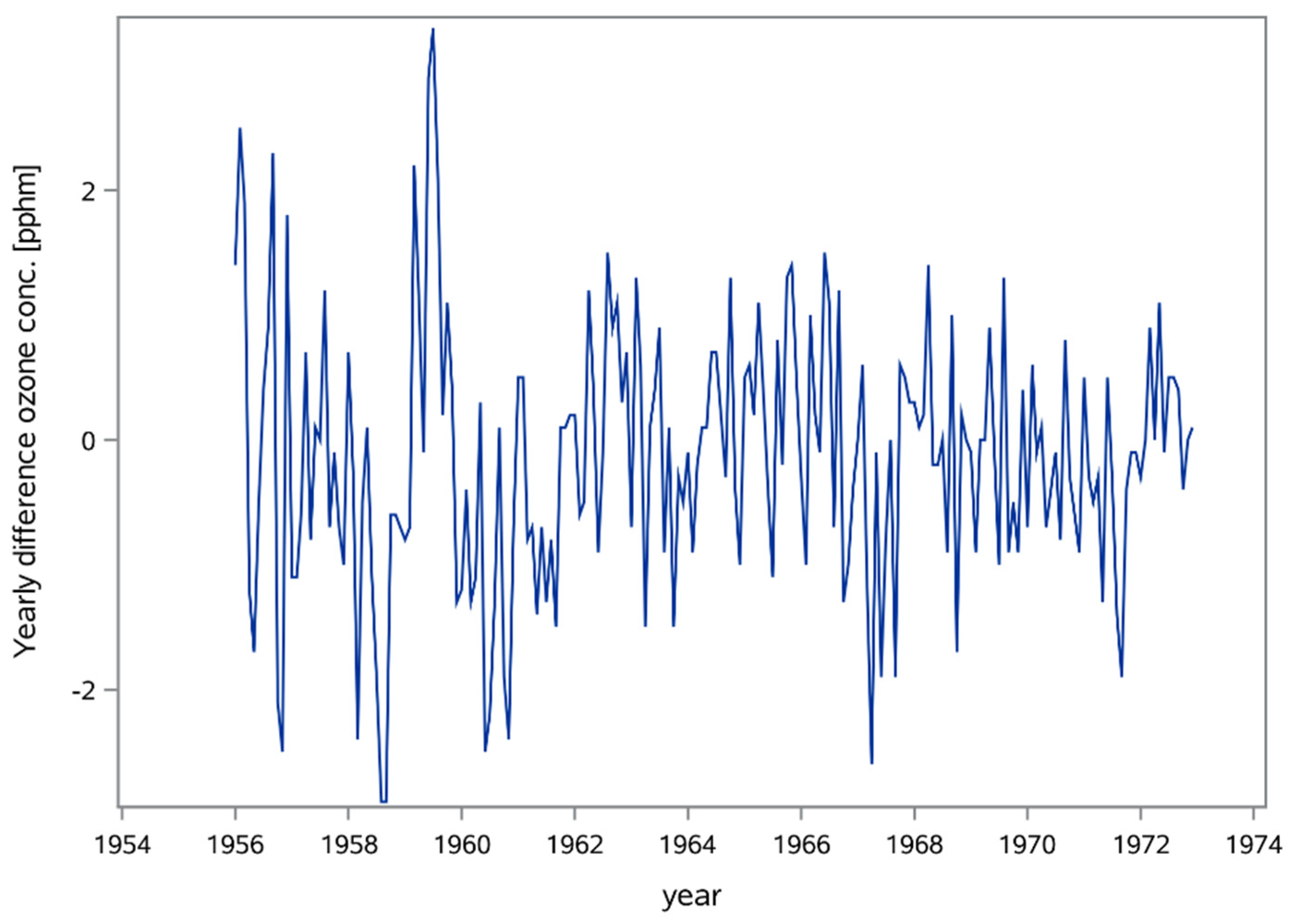
To remove the seasonal variation from the ozone concentration, the ozone series was differenced at lag 12, as was done in the study by Box and Tiao [29]. The value 12 was selected because the data was recorded monthly and the seasonality was annual. The time-series of the ozone level during the time of 1955 to 1973 exhibits a clear seasonal component (Figure 1), which after differencing, disappeared (Figure 2).

Our study starts with the work of Box and Tiao, which used the ARIMA procedure in combination with maximum likelihood (ML) to develop a model for the ozone concentration. However, we will expand their work by including besides ML, parameters of the same model estimated with two additional algorithms: CLS and ULS. We compared the performances of the algorithms with the Akaike Information Criteria (AIC).

We have tested the necessity of using ARIMA by developing the simpler autoregressive model without the moving average term. The autoregressive model explains the current value of the series based only of number p past values, AR (p). Similarly to ARIMA, we investigated the performances of four algorithms in modeling the ozone concentration. The results supplied by each algorithm were compared using the AIC and coefficient of determination (R²).

2.2.1. ARIMA Model and Estimation Algorithms

Box and Tiao [29] reached the conclusion that an ARIMA process (Equation (4)) is suitable for modeling the ozone concentration in downtown Los Angeles:

$$ozone={\beta }_0+{\beta }_{1}x1+{\beta }_{2}Summer+{\beta }_{3}Winter+{\epsilon }_t$$

(4)

where ozone is the concentration of zone in pphm, X1, Summer, and Winter are the intervention variables, and ε is the noise or the stochastic variation.

Box and Tiao used the autocorrelation function to identify the lag needed to eliminate the seasonal behavior of ozone concentration. They found that lag 12 of the ozone leads to a significant correlation at lags 1 and 12 for noise, which prompted the model:

$$\left(1-B_{12}\right){\epsilon }_t=\left(1-{\theta }_{1}B\right)\left(1-{\theta }_2{B}^{12}\right)e_t$$

(5)

where B is the backshift operator of lag 1, such that By_t = y_t−1, e_t is the white noise, namely an independently distributed normal variable with mean 0 and variance σ_a, regardless the time t, θ(B) = 1 − θ₁B − θ₂B² − … −θ_qB^q is the moving average polynomial of order q. The model fitted by Box and Tiao was

$$ozon{e}_t={\beta }_{1}x{1}_t+{\beta }_2\frac{summe{r}_t}{\left(1-B^{12}\right)}+{\beta }_3\frac{winte{r}_t}{\left(1-B^{12}\right)}+\frac{\left(1-{\theta }_{1}B\right)\left(1-{\theta }_2{B}^{12}\right)}{\left(1-B^{12}\right)}{e}_t.$$

(6)

The details of each estimation algorithm are presented in multiple sources [31,32,35,36,37], but in this paper we will just summarize the main aspect of each algorithm. The CLS estimation is conditional on the assumption that past unobserved errors are equal to 0 and it produces estimates by minimizing the Equation (7):

$${\displaystyle \sum }_{t=1}^n{a}_t^2={\displaystyle \sum }_{t=1}^n{(x_t-{\displaystyle \sum }_{i=1}^{\infty }{\pi }_i{x}_{t-i})}^2$$

(7)

where π is computed from the estimates of $\phi$ and $\theta$ at each iteration, which are the AR and MA parameters for the series $x_1,\dots ,x_{t-1},x_t$, and $\sum _{t=1}^n{a}_t^2$ is $e\times e’$ where e is the white noise, and e’ is the transpose of e.

The ULS estimates start from the estimates computed by using CLS algorithm, which are further minimized (Equation (8)):

$${\displaystyle \sum }_{t=1}^n{a}_t^2={\displaystyle \sum }_{t=1}^n{(x_t-C_t{V}_t^{-1}{(x_1,\cdots ,x_{t-1})}^{’})}^2$$

(8)

where C_t is the covariance matrix and $V_t$ is the variance matrix for the series $x_1,\dots ,x_{t-1},x_t$.

The ML algorithm maximizes the likelihood function through nonlinear least square Marquardt’s method (Equation (9)). The initial estimates are computed using the CLS.

$${\left|H\right|}^{\frac{1}{n}}{e}^{\prime }e{\left|H\right|}^{\frac{1}{n}}$$

(9)

where e is white noise vector and H is the lower triangular matrix with positive elements on the diagonal, such that $H{H}^{\prime }=\Omega$ where $\Omega$ is the determinant of the regression equation.

The three algorithms were assessed, with AIC (Equation (10)), which is a measure of the goodness of fit of the model as well as the complexity of that model.

AIC = − 2ln (L) + 2k

(10)

where L is the maximized value of the likelihood function for the estimated model and k is the number of estimated parameters.

2.2.2. Autoregressive Model and Estimation Algorithms

The autoregressive process used to model the time series is:

$$Y_t={X^{\prime }}_t\beta +{\epsilon }_t$$

(11)

where Y_t is the response variable, X’_t is the matrix of predictor variables with β slope, and ε_t is the error term.

For consistency with the ARIMA model, we have considered an autoregression model that includes as predictor X1, summer, and winter (Equation (12)):

$$ozone={\beta }_{1}x1+{\beta }_{2}summer+{\beta }_{3}winter+{\epsilon }_t$$

(12)

where ozone is the predicted and the interventions X1, summer and winter are the predictors.

Cleveland [38] suggested that autocorrelation, inverse auto correlation and partial auto correlation functions should be used to determine the autoregressive order. Using the three autocorrelation functions we found 12 as the lag fulfilling the modeling requirements, confirming the ARIMA approach. To remove the possible correlation among residuals still present after differentiation, we have further differentiated the residuals:

$${\epsilon }_t={\varphi }_1{\epsilon }_{t-1}+{\varphi }_2{\epsilon }_{t-2}+\dots +{\varphi }_l{\epsilon }_{t-l}+e_t$$

(13)

where l is the lag and e_t is white noise.

The final model became:

$${\nabla }_{12}ozone={\beta }_1{\nabla }_{12}x1+{\beta }_{2}summer+{\beta }_{3}winter+e_t$$

(14)

where ${\nabla }_{12}ozone$ and ${\nabla }_{12}x1$ are seasonally differenced at lag 12 for Ozone and X1, respectively.

To estimate the parameters of the autoregressive model 12 we have considered four algorithms: Yule–Walker (YW), Iterative Yule–Walker (ITYW), maximum likelihood (ML), and unconditional least square (ULS).

The Yule–Walker algorithm starts from the ordinary least square estimates of β, which is used to estimates Φ, the parameters of an AR (p) process, from the sample autocorrelation function of the residuals. The equation supplying the $\widehat{\Phi }$ is:

$$\widehat{\Phi }=-R^{-1}r$$

(15)

where $\widehat{\Phi }$ is the vector of autoregressive parameters, r is the vector (r₁, …,r_p), where r_i is the lag i sample autocorrelation, R is the Toeplitz matrix with the elements r_i,j=r_|i-j|.

The Iterative Yule–Walker algorithm uses the resulted residuals stemmed from the YW algorithm to create new estimators of ϕ.

The ML algorithm is based on the likelihood function 16.

$$L\left(\epsilon ,\beta ,{\sigma }^2\right)={\displaystyle \prod }_{i=1}^{n}f\left({\epsilon }_i\right)=\frac{1}{{(2\pi )}^{\frac{n}{2}}{\sigma }^n}{e}^{\left(-\frac{1}{2{\sigma }^2}{\epsilon }^{\prime }\epsilon \right)}$$

(16)

where ε_i are the residuals, β are the parameter, and σ² is the variance of ε.

The likelihood function for an AR(1) model is

$$L\left(\epsilon ,\beta ,{\sigma }^2\right)={(2\pi {\sigma }^2)}^{-\frac{n}{2}}\sqrt{1-{\varphi }^2}{e}^{-\frac{1}{2{\sigma }^2}S\left(\varphi ,\mu \right)}$$

(17)

$$\begin{gathered} S\left(\varphi ,\mu \right)={\displaystyle \sum }_{t=2}^n{\left[\left(y_t-\mu \right)-\varphi \left(y_{t-1}-\mu \right)\right]}^2+\left(1-{\varphi }^2\right)\left(y_1-\mu \right) \\ =S_c\left(\varphi ,\mu \right)+\left(1-{\varphi }^2\right)\left(y_1-\mu \right). \end{gathered}$$

(18)

To maximize the likelihood function, it is customary to execute the computation on the logarithm of L rather than on L, after which partial derivatives are computed in respect with σ². The derivation of likelihood function is in general considerably more involved, which requires estimations with numerical methods.

The ULS algorithm, is a compromise between conditional least square estimates and maximum likelihood, and is focused on minimization of the S(ϕ,μ) (Equation (18)):

Besides AIC, we have assessed the model using the mean square error (MSE) and the coefficient of determination (R²) [39].

$$\mathrm{Mean} \mathrm{Square} \mathrm{Error} MSE={\sum }_{i=1}^n\frac{{(Y_i-{\widehat{Y}}_i)}^2}{n-p}$$

(19)

$$\mathrm{Coefficient} \mathrm{of} \mathrm{determination} R^2=1-{\sum }_{i=1}^n{(Y_i-{\widehat{Y}}_i)}^2/{\sum }_{i=1}^n{(Y_i-\overline{Y})}^2$$

(20)

where $Y_i$,${\widehat{Y}}_i$,$\overline{Y}$ are the actual, the predicted, and the average predicted variable, n is the total number of observations and p is the number of parameters in each model.

We considered the analysis concluded when the residuals of the time series model are white noise, which was tested with the Durbin–Watson test. All computations were executed using SAS 9.4 [6].

3. Results

Our results confirm the findings of Box and Tiao, as all variables included in the ARIMA model were significant (p < 0.001), irrespective the algorithm except for the Winter variable, which was significant only for α = 0.1 (

Table 2. Parameter estimates and fit statistics (mean square error (MSE), and Akaike Information Criterion (AIC)) of the ARIMA (autoregressive integrated moving average) model with three different algorithms of the ARIMA process. CLS—conditional least square; ULS—unconditional least square; ML—maximum likelihood.

Algorithm	Ozone lag (1)	Ozone lag (12)	X1 lag(12)	Summer	Winter	MSE	AIC
CLS	−0.29983	0.59234	−1.2624	−0.2615	−0.082	0.856	520.52
ULS	−0.25264	1	−1.3742	−0.2027	−0.084	0.768	510.78
ML	−0.26684	0.76665	−1.3306	−0.2394	−0.080	0.797	501.77

).

The results suggest that all variables have negative impact on ozone concentration. The highest AIC and SE values, therefore the worse performances, were supplied by the CLS algorithm, which is the default option in SAS. This finding suggests that the default algorithm is not always the best choice for estimation of the parameters defining a model. The best result, according to AIC, was achieved when ML algorithm was used, which explains the choice of Box and Tiao in solving the ARIMA process. However, ULS supplied the smallest mean square error among the tree, suggesting that different criteria could lead to different findings.

We forecasted the year 1973 with 95% confidence interval (Figure 3). For consistency, we predicted the monthly ozone concentration using the same three algorithms: ML, CLS, and ULS (

Table 3. Forecasting the year 1973 using three ARIMA estimation algorithms: CLS, ULS, and ML.

1973	CLS		ULS		ML
Months	Forecast	SE	Forecast	SE	Forecast	SE
January	1.4538	0.8562	1.2738	0.7677	1.4205	0.7966
February	1.8783	0.8938	1.5871	0.7919	1.8446	0.8244
March	2.5705	0.8938	2.2482	0.7919	2.4567	0.8244
April	2.8788	0.8938	2.7649	0.7919	2.8590	0.8244
May	3.1553	0.8938	2.9482	0.7919	3.1501	0.8244
June	2.8074	0.8938	2.7952	0.7919	2.7211	0.8244
July	3.3355	0.8938	3.3341	0.7919	3.3147	0.8244
August	3.4400	0.8938	3.3507	0.7919	3.4787	0.8244
September	2.8253	0.8938	3.2952	0.7919	2.0405	0.8244
October	2.0741	0.8938	2.7507	0.7919	2.3587	0.8244
November	1.6465	0.8938	2.3982	0.7919	1.8588	0.8244
December	1.2149	0.8938	1.5663	0.7919	1.2898	0.8244

). We noticed that the MSE for the forecasted months with the CLS algorithm were the highest among the three algorithms, which is an additional verification that the default option should not always be the preferred estimation choice.

The autoregressive model described by Equation (14) and solved with the four algorithms also revealed the importance of the algorithm in estimation of the parameters (

Table 4. Analysis of the errors produced by the autoregressive model with the four algorithms.

Algorithm	MSE	AIC	R2	Durbin Watson at Lag 12
				Pr < DW	Pr > DW
ML	0.76425	527.862	0.5153	0.4647	0.5353
ULS	0.76311	528.202	0.516	0.3287	0.6713
ITYW	0.77253	529.044	0.51	0.7413	0.2587
YW	0.77311	529.153	0.5097	0.7526	0.2474

). Consequently, the model performance depends on the algorithm chosen to estimates the parameters. The results show that YW algorithm, which is the default algorithm in SAS for the autoregressive processes, had the largest MSE and AIC, whereas ULS the smallest MSE and ML the smallest AIC (Table 4). The AR findings provides another supporting evidence that the ML algorithm could be the best choice, and that Box and Tiao selected the appropriate approach for solving the ozone concentration model. 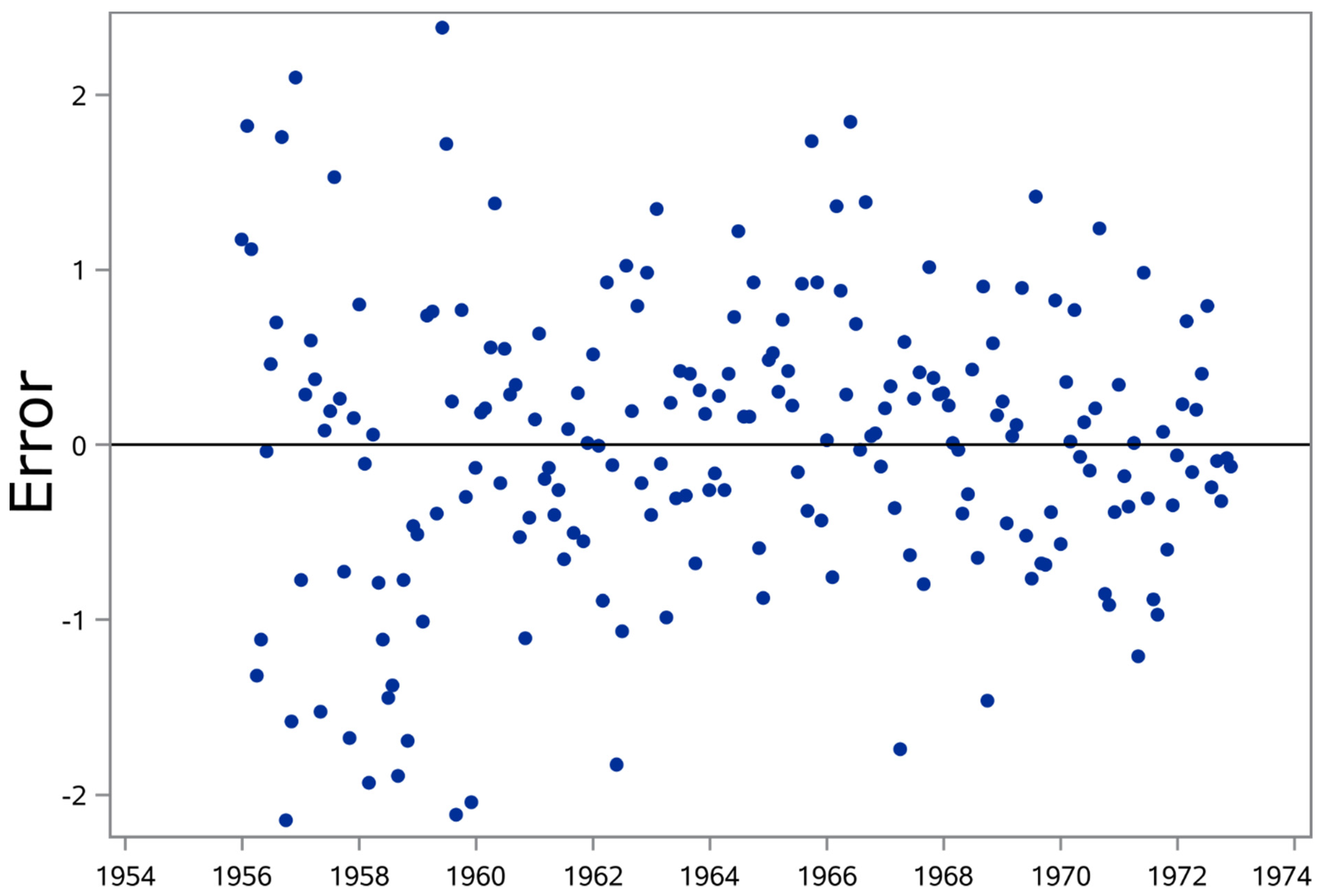The Durbin–Watson test [40] revealed that the errors produced by the autoregressive model 14 are white noise (Table 4). Visual investigation and Durbin–Watson test on the residual produced by the autoregressive model reveals no pattern, and supports their distribution as white noise (Figure 4).

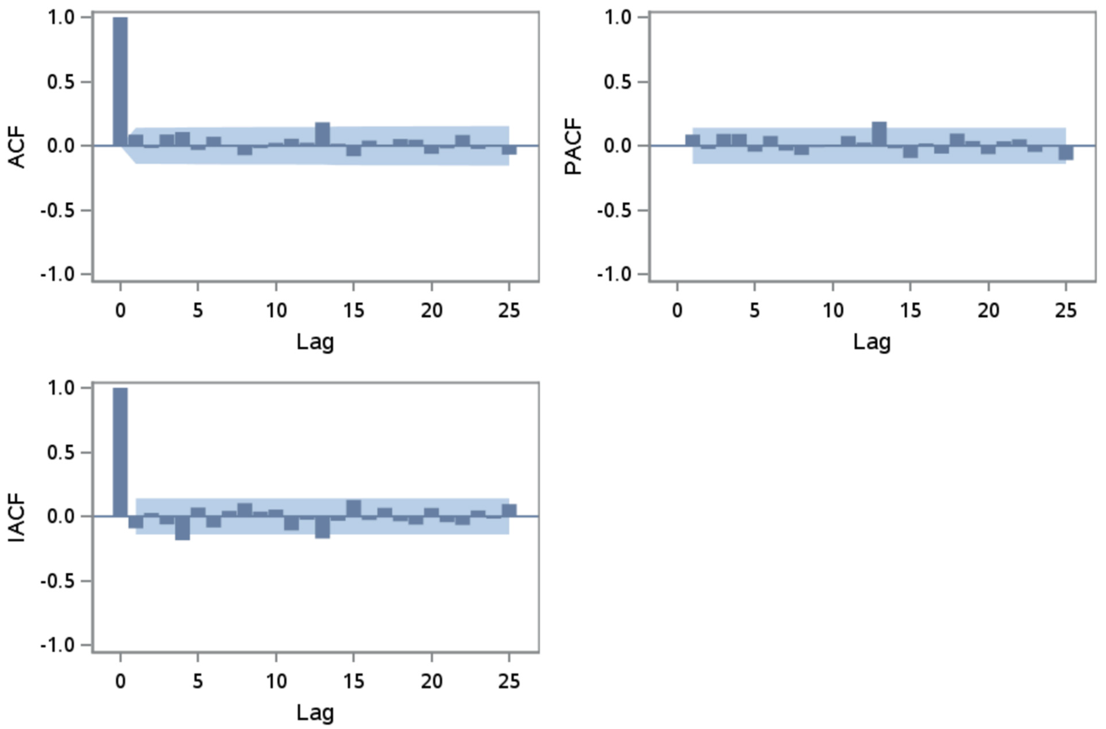
Autocorrelation Function (ACF), Partial Autocorrelation Function (PACF), and Inverse Autocorrelation Function (IACF) support the white noise distribution of the residuals produced by the autoregressive model (Figure 5) and revealed by the Durbin–Watson test (Table 4), as all correlation functions where less than two standard errors. Therefore, the ACF variation suggest that there is no need for additional autoregressive terms whereas the PACF and IACF indicate that there is no need to reduce the model parsimony by including moving average terms in modeling the ozone pollution.

Irrespective of the algorithm, the autoregressive model of Equation 14 produced similar results with ARIMA, in the sense that the winter intervention is not significant (p > 0.5). However, the autoregressive model also shows that the summer intervention is not significant, as the p-value > 0.25. In fact, the autoregressive model shows that the differenced intervention variable is the only significant variable.

4. Discussion

The two modeling approaches of ozone concentration (i.e., ARIMA and autoregressive) lead to models that cannot be challenged based on the achievement of white noise, as both produced the expected distribution of the residuals. However, if AIC was used as a criterion, then the ARIMA supplied superior results then the autoregressive (i.e., 501 vs 527), whereas if MSE is the guiding criterion then the opposite conclusion is reached (i.e., 0.763 vs 0.768). The conflicting findings should be considered in the context of the desired objective, as if the best overall model is needed then the AIC criterion should prevail, while if precise predictions are the focus, then the MSE criterion should be emphasized.

Irrespective of the approach on modeling the ozone concentration, ARIMA or autoregressive, the ML algorithm yielded the best results, according to AIC. However, if MSE is used as criterion, then the ML is not the best, but the least square method is (i.e., ULS for autoregressive models and CLS for ARIMA model), which suggests that for complex models, algorithms that are computational more efficient than ML could be used. Nevertheless, the default algorithms, Yule–Walker for the autoregressive approach and CLS for ARIMA, supplied the worse results, which points toward the necessity of trying various algorithms before reaching a conclusion.

A natural question arises whether ARIMA, a less parsimonious model than AR in term of structure, should be used instead of AR, given that not only similar results are obtained but also ARIMA is an enhancement of AR. The answer lies partially in the criteria used for model selection (i.e., AIC vs. MSE), partially in the overall parsimony, and partially in the predictive ability of the models. Smaller MSE suggests a more performant model, given the central limit theorem, but in the presence of outliers the least square estimator can produce biased results. Furthermore, selection of a model based on MSE offers no warranty that the model is not overfitted [41]. The AIC on the other hand, being based on the likelihood function, not only that is more robust to outliers, but is also an unbiased estimator of the Klluback discrepancy [41], a measure of model agreements. Therefore, in selection of a model, AIC criteria should be preferred over the MSE, as information based criteria consistently supply correct results [42]. In the ozone pollution case the AIC was more than 5% smaller for ARIMA model than the AR model, which suggest the appropriateness of the more parsimonious model (i.e., ARIMA). From the parsimony perspective, ARIMA model uses six parameters whereas the AR model uses five, which suggest the AR as the appropriate model. However, parsimony on itself is not sufficient, most of the time having more a discriminating power rather than being a selective criterion. From the predictive ability perspective, ARIMA is more flexible than AR, because it examines simultaneously the autoregressive part (i.e., variables) and the autocorrelation part (i.e., errors), whereas the AR considers only the autoregressive properties of the time series. Therefore, Box and Tiao selected ARIMA as the model because it meets several desired properties, namely robustness, predictability, and model agreement. However, a stationary process that does not present outliers could be modeled according to the MSE and parsimony, which is the case of AR. Finally, the choice of the model and the algorithm to estimate the parameters defining the model is not unique to ozone pollution or the dataset used in this study. Other studies pointed the importance of the algorithm selection [8,43,44], but not in forestry settings.

The main finding of our study suggests that careless usage of an estimation algorithm, even for simple problems, such as the ozone concentration in downtown Los Angeles that has 216 observations, could lead to questionable results. The conclusion holds irrespective of the approach, simpler, such as autoregressive, or more complex, such as ARIMA. Furthermore, depending on the objective, complex models even superior from some perspectives, could not be appropriate, particularly when considered from the parsimony perspective. Therefore, besides technical details that define the model, operational constraints should be considered, as the AIC should not be applied blindly in model selection.

5. Conclusions

Modeling is considered an area where subjective evaluations are not present, where objectivity rules, which is based on repeatable results. Objectivity and repeatability is of paramount importance for complex models, when not only the accuracy is important but also the precision. However, a model can be developed in multiple ways. Considering that usually models are part of a larger research question, the aim of such studies consists in finding the answer to the question of interest rather than on procedural details. Therefore, technical detail, such as selection of the most appropriate algorithm among the available options, is customarily ignored. Estimation with an inappropriate algorithm could lead to imprecise models, which have cascading effects in complex models such as climate change or pollution. The goal of this study is to compare the solutions supplied by different algorithms used to model a time series, with application to ozone pollution, of significant importance in the current climate change driven paradigm. We have focused on ozone as pollutant to be modeled, as it is important not only for forestry but also for climate change overall. We have used the ozone concentration data from the 1975 study of Box and Tiao, as it is well studied and provides the groundwork to modeling times series data. In addition to the maximum likelihood, which was the algorithm used by Box and Tiao, we have considered two other algorithms to solve the ARIMA process, namely conditional least square and unconditional least square. As an alternative to the ARIMA process, we have modeled the ozone concentration data with a more parsimonious approach, namely an autoregressive process. We have estimated the parameters of the autoregressive model with four numerical algorithms: Yule–Walker, Iterative Yule–Walker, maximum likelihood, and unconditional least square. Irrespective the approach, the ML and ULS produced the most suitable models, within 1% from each other, for MSE, and 5% for AIC. The larger difference in AIC compared with MSE, as well as the robustness to outliers, recommends ARIMA over AR in modeling the ozone pollution. Nevertheless, for a stationary process that is identified using data without outliers an AR model could be more appropriate, as MSE supplied by the ULS algorithm was always the smallest, regardless the model (i.e., 0.763 against 0.764 of ML for AR and 0.768 vs 0.797 of ML for ARIMA).

Our study proves that Box and Tiao’s choice of ML algorithm is the most suitable selection for working on the ozone data from downtown Los Angeles, according to AIC but not according to mean square error criterion. Furthermore, we found that Yule–Walker, which is the default algorithm in many software used for time series modeling, has the least reliable results, suggesting that the method of solving complex models could alter the findings. Finally, the model selection depends on the technical details as well as on the applicability of the model, as ARIMA model is suitable from AIC perspective but an autoregressive model could be preferred from mean square error viewpoint.

The present study proposes indirectly a procedure of selecting the algorithm that would produce the most appropriate results. However, the main limitation of the presented approach is the requirement to run multiple algorithms for multiple models, which, in eventuality of large dataset as inputs, could become time consuming. Therefore, future research should focus on the search of the algorithm that fits the model, the data, and the evaluation criteria.