Estimation of Uncertainty in Airborne LiDAR Inventories Using Approaches Based on Bootstrapping-Pairs Methods

Abstract

LiDAR inventories were carried out to estimate the mean volume and variance in Eucalyptus globulus and Eucalyptus nitens stands. Uncertainty of the population estimates was examined using approximations based on the bootstrap method. Three methods were tested, the traditional bootstrapping-pair method (Method 1) and two additional methods in which the residual variance of the models was incorporated. Method 2 incorporated the residual variance in homoscedastic structure and Method 3 incorporated the heteroscedastic residual variance. Bootstrapping-pairs based on Method 3 generated similar estimates for the mean volume and slightly higher estimates for the variance as the traditional method (Method 1). Variance estimates obtained with the traditional bootstrapping-pairs method could be biased due to the presence of heteroscedasticity. Method 3 was found to best estimate the variance of the mean volume in LiDAR inventories, when the models that describe the relationship between stand variables and LiDAR metrics do not meet the assumption of homoscedasticity. It is shown that the uncertainty of the estimation of the average volume decreased in stands with a larger area, stabilizing the uncertainty of estimates in stands with areas larger than 50 hectares. Our results suggest that the residual variance in the heteroscedastic structure must be incorporated to avoid bias when bootstrapping-pairs are used in small area stands (less than 5 hectares).

1. Introduction

In the last decades, LiDAR technology has been widely used in forestry to provide support for forest management and has been used as a support tool for forest inventories [1,2]. The advantages of using this technology in forest inventories have been described by numerous authors, who have mainly agreed that in large areas and with high forest variability, LiDAR technology provides better estimators than traditional inventories with a shorter execution time and reduced associated costs [1,2,3,4,5,6]. Furthermore, inventories using LiDAR may be the only economically feasible way to estimate the stand variables in a forest with rough terrain [7,8].

Traditional and LiDAR inventories are tools that assist evaluating forests by estimating their variables at the population level. In traditional inventories, the inference is constructed from the assignment of the sampling plots under a probabilistic design within a defined study area [9]. Thus, the estimates of the population parameters of interest are made based on a known design, which defines the way of calculating the mean and its variance; these estimates being constant for the entire study area [10]. In the LiDAR inventory, the estimation of variables is made from models that have been previously calibrated, which consists of the construction of functions that relate the stand variables measured in plots with metrics obtained from the LiDAR point cloud. From here, these models are used to estimate the attributes of the forest, using LiDAR metrics as auxiliary variables that explain stand density, height, basal area, total and commercial volume, among others [1]. The use of LiDAR’s metrics measured in the whole population is considered as auxiliary information and in statistical inference it has been used mainly to improve the accuracy of the population estimates [5]. In addition, in forest inventories, the use of auxiliary information obtained from LiDAR technology is considered economically more efficient in collecting auxiliary information that could be generated from traditional measurements [11].

The effect of incorporating auxiliary variables from LiDAR on the models used to make population estimates improves the precision of the estimates because the models show greater variability in the forest. Næsset [12] reported that between 80 and 93% of the variability of the volume measured in the field could be explained by models that use LiDAR information as an auxiliary variable. Others have reported that 88% of the variability of the aerial biomass is explained with models that use LiDAR’s metrics [13]. The main advantage of using auxiliary variables with respect to the traditional estimates is that model-based estimators generate estimates for each of the population elements, these being more precise in stands where the forest is highly variable or where it is not possible to establish an adequate number of measurement plots [14,15,16,17]. These advantages are even more evident in small and difficult to access stands [17]. Meanwhile, the main disadvantage is that the estimates are not necessarily unbiased and often require heavy computational expense depending on the size of the study area and the required inventory resolution [18].

In model-based inference, the quality of population estimates depends on the model’s ability to capture and represent stand variability [8,11]. This technique allows the use of samples external to the study area in the modeling phase, unlike traditional inventories, where the inference is usually based on the sampling design within the study area. Because of this, the model-based inference is more flexible and attractive for estimating forest inventories in which auxiliary information of the population is available. Thus, model-based estimates using LiDAR’s metrics like an auxiliary variable allows the estimation of the average and its variance in more precisely defined areas [19]. However, despite the flexibility provided by model-based estimation methods, its implementation should give special emphasis to the statistical properties of the models, since population estimates depend on the quality of the fit, bias of the model, its predictive capacity and ability to represent the variability of the forest given by the auxiliary variables [19]. Thus, when the inference in sampling is based on models, the uncertainty of population estimates depends to a greater extent on the predictions made by the model and its residual variance [11,20].

In forest inventories the model-based inferences that use LiDAR auxiliary information, present several challenges since the sample is not probabilistic. Thus, the main challenge is obtaining the variance of the estimator of the population mean, since this consists of the covariance terms of the prediction, residual variance of the model and the covariance of residuals given the spatial distribution component. McRoberts, et al. [8] described each of the equations required to determine the above terms. They also mention that a valid alternative to generate the approximations of the variance of the population mean is the implementation of the technique known as “bootstrapping-pairs” described by Efron and Tibshirani [21]. There are several studies that have implemented this technique [8,11,16,20], however, only in McRoberts, et al. [8] has the importance of including the residual variance in bootstrap cycles been mentioned and with even greater relevance when the model does not meet the assumption of homogeneous residual variance. Thus, the hypothesis is that the incorporation of residual variance of the model in the bootstrapping process will generate a better estimator of the population variance. In our research, estimates of the variance of mean volume were generated in operational stands of E. globulus and E. nitens in different areas, implementing three methods: the traditional bootstrapping-pairs method, a modification of the bootstrapping method that incorporates the homoscedastic residual variance and another that incorporates the heteroscedastic residual variance, both simultaneously modeled by maximum likelihood method.

2. Materials and Methods

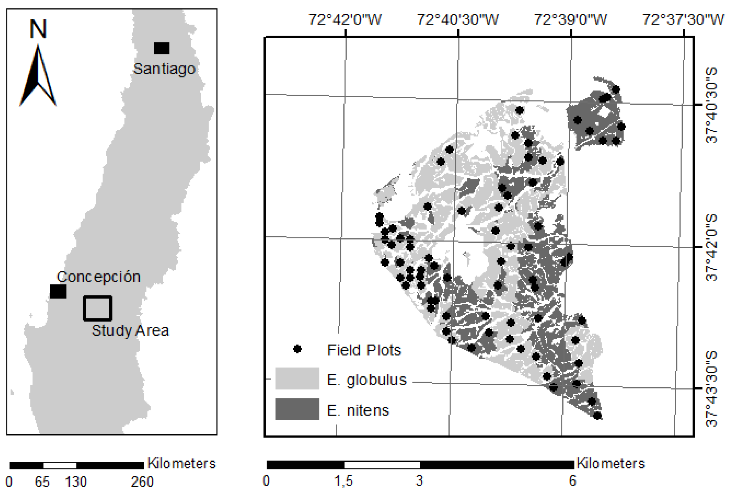
2.1. Data

Data corresponds to a LiDAR inventory carried out in the commune of Angol, between the limits of the Biobío and La Araucanía region, Chile. 34 stands of E. globulus and 10 stands of E. nitens were evaluated in stand ages comprised in the range of 10 to 12 years. The total evaluated area was 1290 hectares, with stand areas between 1 and 248 hectares for E. globulus and between 0.5 and 414 hectares for E. nitens (Figure 1). The inventory was planned as an operational inventory by the company Forestal Mininco S.A.

In the LiDAR modeling, 52 sampling plots were used for E. globulus and 51 plots in E. nitens. The sampling plots were established in the field according to the variability in forest height determined from the LiDAR information. The height data was grouped into five height classes, and in each class the sampling plots were randomly assigned to cover the full variability of the stands. All the plots were circular with a surface area of 500 m², in which were measured the total height, dominant height, basal area, stocking, total and commercial volume. The center of each plot was determined with a Trimble R1 model 99,133 submetric precision GPS (Trimble Inc., Sunnyvale, CA, USA). The LiDAR data were captured in October 2019, at the same time that the traditional inventory was carried out with field measurements. The LiDAR sensor used was the Trimble Harrier 68i model (Trimble Inc., Sunnyvale, CA, USA) with 400 kHz laser and a firing speed of 200 Hz. The sensor was mounted on a Cessna aircraft with a flight height of 900 m above ground level, strip width was 800 m, LiDAR sidelap was 25%, average speed of the aircraft 198 km/hr, which generated an average density of 6 points/m². Processing with LAStools software [22] was used to classify the returns of the LiDAR point cloud corresponding to soil and vegetation, obtaining the normalized height model and LiDAR metrics in each of the study stands, while FUSION/LDV [23] was used to obtain LiDAR metrics at the level of the sampling plots.

The surface of each stand was discretized in units given by a pixel of 500 m² defining each pixel as $U=\left\{1,2,\dots ,N\right\}$. This resolution also reflects the resolution of the auxiliary variables given by the LiDAR metrics. The plots used for the modeling in each species were 500 m², which were established in a representative network and spread throughout the study area under a sampling design with selection probability $p(s)$; here all the sampling units ($s$) are within the stands studied ($s\in U$).

2.2. Method Development

Population estimators for the average ${\mu }_y$ generated from model-based inference can be written in their generalized form (Equation (1)).

$${\widehat{\mu }}_y=\frac{1}{n}{\displaystyle \sum _{i\in s}\left(y_i-f(\widehat{\beta }|X_i)\right)}+\frac{1}{N}{\displaystyle \sum _{i\in U}f(\widehat{\beta }|X_i)}.$$

(1)

where $\widehat{\beta }|X_i$ is the estimate value for the $y_i$ given the auxiliary variable $X$ in the model. Thus, ${\widehat{\mu }}_y$ is the mean of estimated values in the population $1/N{\displaystyle \sum _{i\in U}f(\widehat{\beta }|X_i)}$ and the mean of the errors generated by the model at the sample level $1/n{\displaystyle \sum _{i\in s}\left(y_i-f(\widehat{\beta }|X_i)\right)}$. Meanwhile, the variance of the estimator of population mean is described as $V({\widehat{\mu }}_y)=E{({\widehat{\mu }}_y-E({\widehat{\mu }}_y))}^2$, and the expected value of the mean for the sampling design is $E({\widehat{\mu }}_y)={\displaystyle \sum _{s\in U}{\widehat{\mu }}_y^{(s)}p(s)}$. Hence the unbiased estimator of variance can be obtained using the expansion of Taylor series to approximate the estimator of the variance of ${\widehat{\mu }}_y$ by the Equation (2).

$${\widehat{V}}_{\widehat{\mu }}=\left(1-\frac{n}{N}\right)\frac{1}{n}\frac{1}{N-1}{\displaystyle \sum _{i\epsilon U}{\left(y_i-{\beta }_U|X_i\right)}^2}.$$

(2)

According to McConville, et al. [24], Equation (2) tends to underestimate the real variance as the model incorporates more predictors, although this allows the models to better represent the real variation of the population. In this case ${\beta }_U$ is the vector of parameters at the population level which is unknown, also this variance estimator cannot be calculated since the $y$ values are only known in sample $s$. However, according to sampling theory, Equation (2) can be simplified using only the sample components. Thus, the estimator can be expressed by averaging the residual squares of the sample (Equation (3)).

$${\widehat{V}}_{\widehat{\mu }}=\left(1-\frac{n}{N}\right)\frac{1}{n}\frac{1}{n-1}{\displaystyle \sum _{i\epsilon s}{\left(y_i-f\left({\widehat{\beta }}_s|X_i\right)\right)}^2}.$$

(3)

This estimator is asymptotically unbiased, but as described in McConville, et al. [24], tends to underestimate the real variance of the average since it does not incorporate the residual variance of the model. McConville and Breidt [25] demonstrated that, when the number of predictors in the model increases, the variance estimator decreases generating an estimator with negative bias. To avoid that effect in our research the variance of ${\widehat{\mu }}_y$ was estimated using the bootstrapping-pairs method [8,11,18,19,24]. This approach to non-parametric estimation of variance, described by Efron and Tibshirani [21], uses the variability of the estimator ${\widehat{\mu }}_y$ given by the probability sample $p(s)$ in order to determine the variance estimator $V_{\widehat{\mu }}$. According to Mashreghi, et al. [26] this procedure generates an unbiased estimator to $V_{\widehat{\mu }}$ using the variability introduced by a random re-sampling with replacement. Estimators of mean (${\tilde{\mu }}_y^{(B)}$) and variance (${\tilde{V}}_{\tilde{\mu }}^{(B)}$) by the bootstrapping-pairs method were calculated from (Equation (4)):

$${\tilde{\mu }}_y^{(B)}=\frac{1}{B}{\displaystyle \sum _{b=1}^B{\widehat{\mu }}_y^{(b)}}$$

(4)

where the population mean in the $b$-th bootstrap iteration is (Equation (5)):

$${\widehat{\mu }}_y^{(b)}=\frac{1}{n}{\displaystyle \sum _{i\in s}\left(y_i^{(b)}-f({\widehat{\beta }}^{(b)}|X_i^{(b)})\right)}+\frac{1}{N}{\displaystyle \sum _{i\in U}f({\widehat{\beta }}^{(b)}|X_i)}.$$

(5)

where $1/n{\displaystyle \sum _{i\in s}\left(y_i^{(b)}-f({\widehat{\beta }}^{(b)}|X_i^{(b)})\right)}$ is the mean of the errors generated by the model at the sample level in the $b$-th bootstrapping iteration, and $1/N{\displaystyle \sum _{i\in U}f({\widehat{\beta }}^{(b)}|X_i)}$ is the mean of the estimated values in the population using the parameterization of the model in the $b$-th bootstrap iteration. Thus, the estimate variance of ${\tilde{\mu }}_y^{(B)}$ is:

$${\tilde{V}}_{\tilde{\mu }}^{(B)}=\left(\frac{n}{n-1}\right)\left(\frac{N-n}{N-1}\right)\frac{1}{B-1}{\displaystyle \sum _{b=1}^B{\left({\widehat{\mu }}_y^{(b)}-{\tilde{\mu }}_y^{(B)}\right)}^2}$$

(6)

In our investigation, the bootstrapping resample number was defined in 1000 considering the suggestion made by Puliti, et al. [11]. Equation (6) generates the estimator of the variance of ${\tilde{\mu }}_y^{(B)}$ considering the error term given by bootstrap sampling and sampling design with selection probability $p(s)$. In those equations the fitted regression model assumes error distribution ${\epsilon }_i\sim N\left(0,{\sigma }^2\right)$, however, homoskedasticity in general does not occur when estimating stand variables based on LiDAR metrics [27]. In this investigation, the residual variance of the model was incorporated as another source of variation in the population estimators. Thus, Equations (4) and (6) which estimate the mean ${\tilde{\mu }}_y^{(B)}$ and variance ${\tilde{V}}_{\tilde{\mu }}^{(B)}$ were modified as:

$${\stackrel{⌣}{\mu }}_y^{(B)}=\frac{1}{B}{\displaystyle \sum _{b=1}^B{\widetilde{\stackrel{⌣}{\mu }}}_y^{(b)}}$$

(7)

$${\widetilde{\stackrel{⌣}{\mu }}}_y^{(b)}=\frac{1}{n}{\displaystyle \sum _{i\in s}\left(y_i^{(b)}-f({\widehat{\beta }}^{(b)}|X_i^{(b)}\pm {\sigma }_{}^{(m)})\right)}+\frac{1}{N}{\displaystyle \sum _{i\in U}f({\widehat{\beta }}^{(b)}|X_i\pm {\sigma }_{}^{(m)})}$$

(8)

$${\stackrel{⌣}{V}}_{\stackrel{⌣}{\mu }}^{(B)}=\left(\frac{n}{n-1}\right)\left(\frac{N-n}{N-1}\right)\frac{1}{B-1}{\displaystyle \sum _{b=1}^B{\left({\widetilde{\stackrel{⌣}{\mu }}}_y^{(b)}-{\stackrel{⌣}{\mu }}_y^{(B)}\right)}^2}$$

(9)

Equation (7) represents is the general average of the process ${\stackrel{⌣}{\mu }}_y^{(B)}$, considering the $m$-th assignment of the residual variance of the model ${\sigma }^{(m)}$ with normal distribution ${\epsilon }_i\sim N(0,{\sigma }^2)$. In this way the value of each pixel was generated from the function and term of residual variance as $f({\widehat{\beta }}^{(b)}|X_i\pm {\sigma }^{(m)})$. This assignment was made in each $b$ bootstrap iteration for the population mean ${\widetilde{\stackrel{⌣}{\mu }}}_y^{(b)}$ in Equation (8) and for the estimator variance ${\stackrel{⌣}{V}}_{\stackrel{⌣}{\mu }}^{(B)}$ in Equation (9).

2.3. Modeling

Because in operational forest inventories the variable of greatest interest is volume, the evaluation of the proposed methods was carried out only for commercial volume. In this research, the commercial volume of each of the species was estimated with two models of non-linear structure widely used and reported in literature [28,29].

$$y_i={\beta }_1{p}_{95}{}^{{\beta }_2}co{v}^{{\beta }_3}+{\epsilon }_i$$

(10)

$$y_i=\frac{\alpha }{1+\exp \left({\beta }_1+{\beta }_2{p}_{95}+{\beta }_{3}cov\right)}+{\epsilon }_i$$

(11)

Equation (10) which will be referred to as Model 1, has a slope and a power parameter, while Equation (11), referred to as Model 2 incorporates a double asymptote to ensure that the estimates are in a defined range. In these equations $y_i$ is the commercial volume of the i-th plot, both $p_{95}$ and $cov$ are LiDAR metrics (percentile 95% of height distribution at the pixel level and ratio of first returns to the number of total returns, respectively); $\alpha$ and ${\beta }_j$ are regression parameters of the model and ${\epsilon }_i$ is the random error. In this study the value of the residual variance $\sigma$ was randomly assigned in each simulation m in two structures. First, it assumed homoscedasticity ${\epsilon }_i^{(m)}\sim N(0,{\sigma }^2)$ and here ${\sigma }^{(m)}=RMS{E}^{(b)}$. Second it assumed heteroscedasticity ${\epsilon }_i^{(m)}\sim N(0,{\sigma }_i^2)$ and here the residual variance was estimated simultaneously in the model fit process using the function $f(\sigma )={\theta }_1{p}_{95}{}^{{\theta }_2}$; where ${\theta }_1$ and ${\theta }_2$ are parameter estimates. Thus, three methods of approximating the variance of the estimated volume ${\widehat{V}}_{\widehat{\mu }}$ were evaluated. In Method 1 the estimation was performed with the traditional bootstrapping-pairs procedure, Method 2 random assignments of the residual variance in homoscedastic structure were made and Method 3 residual variance values were randomly assigned with the heteroscedastic structure modeled in $f(\sigma )$. Models with both error structures were fit using maximum likelihood in the method quasi-Newton Broyden–Fletcher–Goldfarb–Shanno-Algorithm (BFGS) implemented in R software [30]. For the fit of the models, we created a function to optimize the maximum likelihood function in order to find the parameters of the prediction model and the residual variance model simultaneously. The interpretation of ${\widehat{V}}_{\widehat{\mu }}$ was made under the concept “estimation of uncertainty” of ${\widehat{\mu }}_y$, calculated as $\sqrt{{\widehat{V}}_{\widehat{\mu }}}/{\widehat{\mu }}_y·100\%$.

3. Results

3.1. Models Performance

In E. globulus Models 1 and 2, used in each of the three bootstrapping methods, generated similar estimates with similar RMSE (

Table 1. Parameters estimated in the two regression models analyzed for E. globulus and E. nitens. Parameters value corresponds to the average of the 1000 iterations in each bootstrapping-pairs process.

Model	Method	$\mathit{\alpha }$	${\mathit{\beta }}_1$	${\mathit{\beta }}_2$	${\mathit{\beta }}_3$	$\mathit{s}\mathit{d}(\mathit{\alpha })$	$\mathit{s}\mathit{d}({\mathit{\beta }}_1)$	$\mathit{s}\mathit{d}({\mathit{\beta }}_2)$	$\mathit{s}\mathit{d}({\mathit{\beta }}_3)$	${\mathit{\theta }}_1$	${\mathit{\theta }}_2$	RMSE (m3/ha)
E. globulus
1	1		0.0770	1.5303	0.8342		0.2720	0.1954	0.1971			22.8
	2		0.0772	1.5304	0.8339		0.3846	0.1995	0.2072			22.8
	3		0.0632	1.5415	0.8480		0.1934	0.2102	0.1887	21.6170	0.0330	21.7
2	1	216.4260	5.8486	−0.2275	−0.0262	13.8212	1.3731	0.0524	0.0098			22.2
	2	216.4229	5.8464	−0.2265	−0.0265	13.7925	1.3586	0.0566	0.0098			22.2
	3	217.2242	5.9792	−0.2301	−0.0276	22.3504	1.4129	0.0578	0.0098	42.3884	−0.1546	21.9
E. nitens
1	1		0.3080	1.5217	0.4918	0.7323	0.9643	1.3233				34.2
	2		0.3004	1.5437	0.5419	0.3068	0.1525	0.1611				34.1
	3		0.1594	1.5830	0.6602		0.2043	0.1234	0.1785	3.2637	1.3250	32.4
2	1	267.7107	3.5054	−11.1531	−43.0304	12.4449	0.0369	0.8298	3.3628			85.7
	2	266.8452	3.5065	−11.1256	−42.9084	11.9852	0.0343	0.7606	3.1181			86.0
	3	319.4280	8.4594	−0.3437	−0.0495	34.7860	4.8668	0.7278	0.2793	0.3066	2.5574	71.1

$\alpha$, ${\beta }_1$, ${\beta }_2$ and ${\beta }_3$ are the parameters estimates of the prediction function; ${\theta }_1$ and ${\theta }_2$ parameters of the residual variance function. sd() denote standard deviation given by the bootstrapping-pairs process. All the parameters were significant.

). In E. globulus Models 1 and 2 with homoscedastic variance (Method 1 and 2) RMSE values of 22.8 and 22.2 m³/ha were obtained, respectively. With both Models (1 and 2) incorporating heteroscedasticity (Method 3) the RMSE improved, from 22.8 to 21.7 m³/ha in Model 1, and from 22.2 to 21.9 m³/ha in Model 2. Meanwhile, in E. nitens Model 2 did not generate accurate estimates even though the parameters converged. Here Model 2 generated RMSE between 71.1 and 86 m³/ha, much worse than model 1, which had RMSE values between 32.4 and 34.2 m³/ha. In E. nitens lower RMSE values were also found in the Model that incorporates heteroscedastic variance (Method 3). Thus, in both species, the implementation of the three bootstrapping-pairs Methods was carried out with Model 1 considering that it showed better performance.

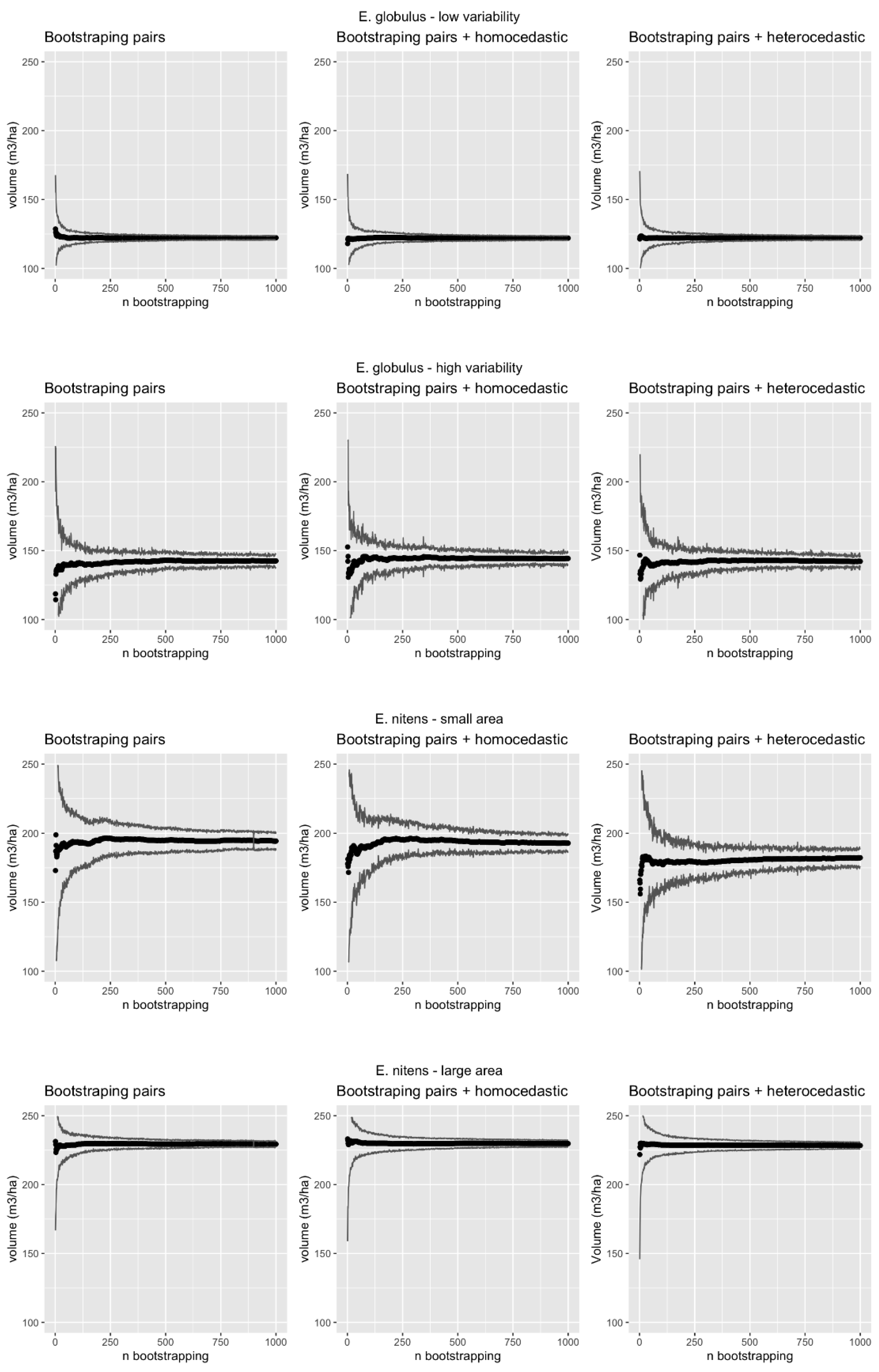
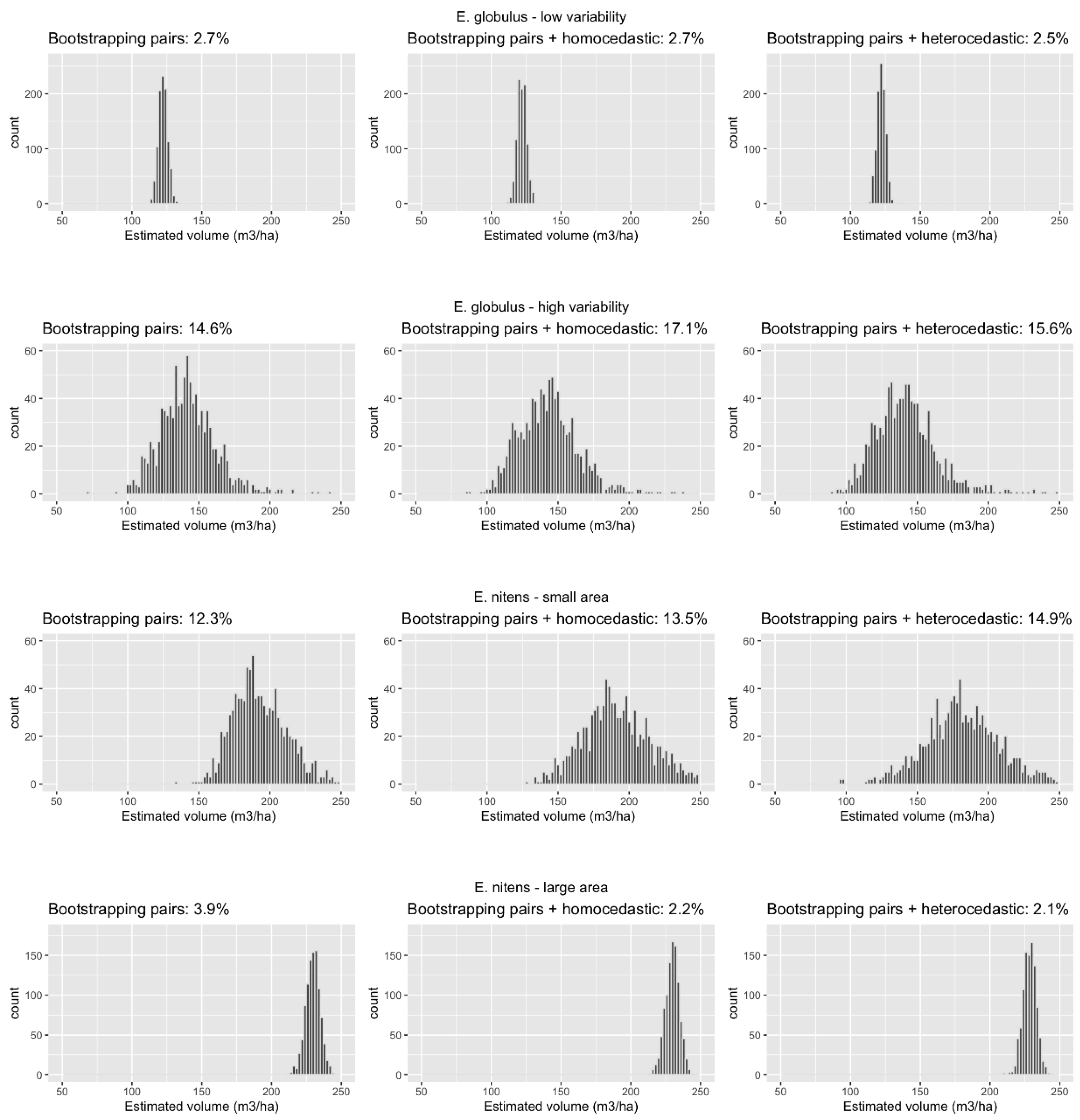
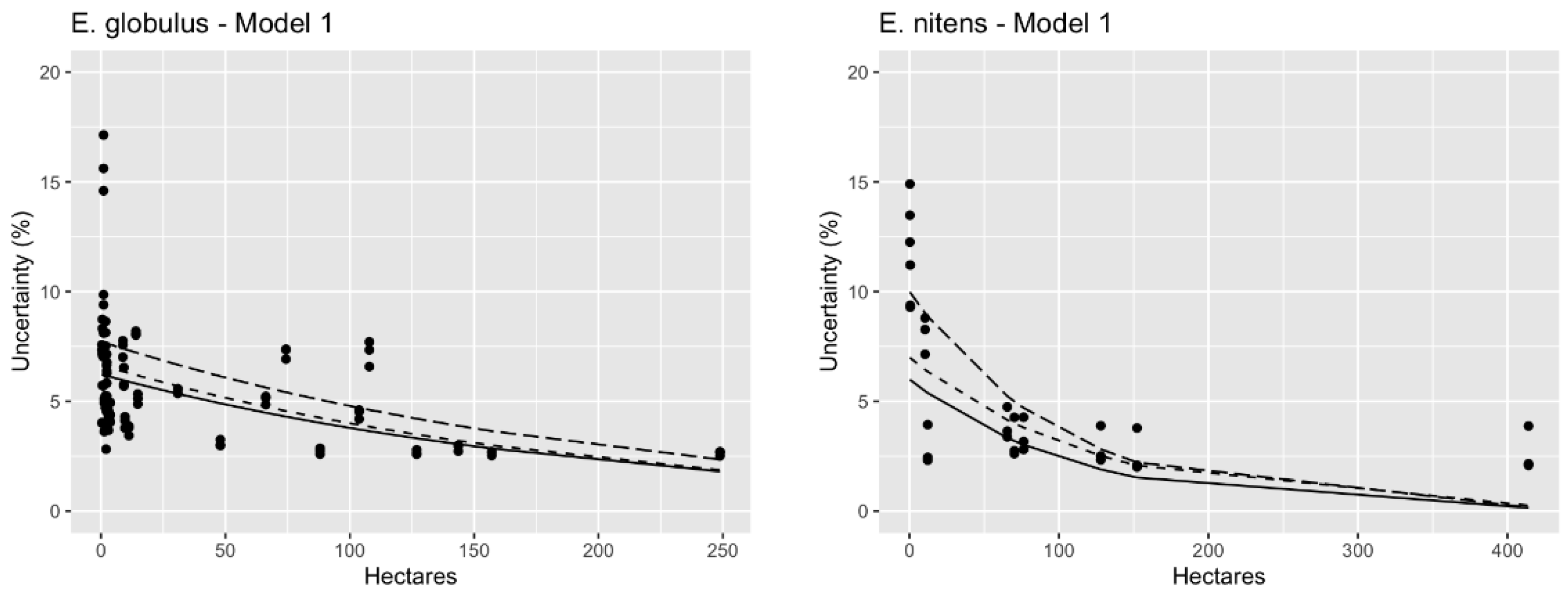
3.2. Methods Performance

In each of the stands, the approximations of the mean volume and variance achieve convergence close to 500 iterations in bootstrapping Methods (Figure 2). In the example of the 1 hectare of E. globulus stand with low variability on pixels, the convergence of the mean volume and variance was achieved between 200 and 250 iterations, while for the 248 hectares stand with high variability on the pixels, the convergence was achieved after 500 iterations. In the example for E. nitens for the small area stand (0.5 ha) the convergence of the estimator of the mean volume and variance was achieved after close to 500 iterations, while in the stand with the largest area (414 ha), convergence was achieved after around 250 iterations. In addition, in the small 0.5 ha stand it was observed that the average volume estimate differed between the three Methods (Figure 2). For the small stand of E. nitens in Method 3 the mean volume estimate is lower than the estimates of Methods 1 and 2, mainly due to the lower value of parameter ${\beta }_1$ in Method 3. In the case of the largest stand of E. nitens this effect does not occur since the number of pixels involved in the calculation of the average volume is large and this allows generating consistent results among the three Methods. This shows that in small stands the effect of the estimation model and the incorporation of its residual variance in the bootstrapping process substantially affects the mean and variance estimates. This effect could be even greater if there is also high variability between pixels in this type of stand, as is the case in stands that have been left as harvest leftovers, protection strips or stand fragmentation after forest fires.

Thus, in general, the convergence of the mean and variance for all stands was obtained between approximately 250 and 500 iterations. Convergence depends on the variability of the stand given by the variability of the LiDAR metrics; in this research the metrics p95 and cov were used. The convergence of the average and its variance depends on the variability of the stand that is collected by the LIDAR metrics, conditioned to the area of the stand. In this research for the stands with similar area with high variability among their pixels, convergence was achieved between 300 and 500 iterations. Based on these results, it could be affirmed that convergence is achieved in bootstrap re-sampling cycles of 500 iterations. This result is important since this process requires a large computational cost-time, and in the context of its implementation in large-scale or operational inventories, this cost-time is significant since the volume of LiDAR information is generally large.

The distribution of the estimated mean volume in the three bootstrapping methods showed a normal distribution in the selected examples (Figure 3). Methods 2 and 3, where the residual variance was incorporated in the prediction of the volume at the pixel level, did not significantly increase the variability of the estimated volume in the stand over that by Method 1. In the example described for Method 3, the increase was highest in the E. nitens stand of 0.5 ha (Figure 3). Here, the estimation uncertainty of the average volume increased from 12.3 to 14.9% relative to that by Method 1. In that same example, Method 2, that incorporated the homoscedastic residual variance, the estimation of uncertainty was 13.5%. In general, the estimation of uncertainty of the volume is lower in Method 3 than by Method 2. In the examples indicated in Figure 4, only in the case of the small stand of 0.5 ha in E. nitens that trend is not met, however, this result could be influenced by the small size of the stand (only 10 pixels). Thus, in general the estimation of uncertainty using Method 3 is lower than Method 2, but higher than that obtained with Method 1. However, we believe that the incorporation of the heteroscedastic residual variance in Method 3 is the most appropriate in the presence of heteroscedasticity, determining more realistic estimation of uncertainty which in turn could be considered more conservative than the traditional bootstrapping-pairs method.

As the area of the stands increases, the uncertainty of volume estimate tends to decrease and this was observed in the three bootstrapping approximation Methods for the two species (Figure 4). The uncertainty of estimation of the volume with Model 1 for the 34 stands of E. globulus was between 2.5 and 17.1%, and for E. nitens between 2.1 and 14.9%, showing the lowest values of uncertainty in the stands with the largest area. The bootstrapping-pairs estimates generated with Methods 1 and 3 were very similar, but in Method 2, which incorporated homoscedasticity, the greatest uncertainty in the estimates was generated and this result is even greater in small stands. In the larger stands, the uncertainty of the estimates tends to stabilize because the number of pixels involved in calculating the estimators is large. Thus, in small area stands (apparently smaller than 5 hectares), the average volume estimate showed higher variability than in larger area stands. Considering this effect, we believe that the incorporation of residual variance in bootstrapping-pairs approximations is recommended when heteroscedasticity is present.

4. Discussion

Despite being a more complex model and with one more parameter to estimate, in E. globulus the double asymptote model (Model 2) gave similar RMSE to those by the non-linear power model (Model 1). Model 2 in E. nitens generated much higher estimation errors than Model 1. Rahlf, et al. [29] reported that the precision of a double asymptote model was similar to that obtained with a model of k-Nearest Neighbors (kNN). The advantage of this model is due to the ability to restrict the range of its estimates given its two asymptotes, but that causes loss of flexibility and prediction ability. McRoberts, et al. [28] generated estimates in a post-stratification forest, where they evaluated linear models, a kNN model and the double asymptote model, highlighting the predictive capacity of the model and that this model avoids having estimates outside the range and negative values which may happen with the estimates using linear models. A similar model to the power model has been used in the research of Martín-García, et al. [16], where they modeled the volume of Pinus radiata only using the height percentile 70 obtaining a RMSE of 18%. In the previous work, the researchers mention that the model meets the assumptions of homoscedasticity, however, only 25 plots were used in modeling the volume established in a homogeneous area. Gobakken and Naesset [31] used a power function model similar to that presented in this study, where they obtained good results when using the height metrics 50 and 90; here homoscedastic residual variance was assumed. In this research, operational measurement plots were established to measure the variability of the stands given by different ages and growth conditions, generating the best results according to RMSE in the models with heteroscedastic residual variance.

In this research, the convergence of the mean volume was achieved after 300 iterations and in the case of the variance after 500 iterations in the bootstrap approximations. Puliti, et al. [11] determined the variance estimator uncertainty according to the traditional bootstrapping-pairs method with 1000 iteration cycles, highlighting that they are sufficient to achieve the convergence of the mean and variance estimators. McRoberts, et al. [8] realized approximations of the estimate of the population variance with the traditional method of bootstrapping-pairs, not mentioning the number of bootstrap cycles, however, they emphasize that it must be performed until the convergence of the mean and variance is achieved. In the work of Martín-García, et al. [16] the estimator variance was determined with 10 thousand bootstrap cycles which we think is an excessive number considering the implementation at the operational level or used in stands of large areas. In the simulation carried out by McConville, et al. [24], 5000 bootstrap cycles were generated, showing that the variance stabilizes after 2000 cycles. In our work, various conditions of stands on different surfaces were evaluated, and in all cases 1000 cycles of the bootstrapping-pairs method were sufficient to achieve convergence of the mean and variance.

In general, the estimation of the volume within the population has been using models without considering the effect of the residual variance at the pixel level. McRoberts, et al. [8] mentioned that the residual variance of the model can be ignored without generating large biases but conditioned to make estimates in large areas. Although the minimum size of that area is not mentioned in that study, the researchers declare that when heteroscedasticity exists, the effect of the residual variance must be incorporated in the estimations. In McRoberts, et al. [8] the heteroscedastic residual variance was incorporated into a linear model ($\widehat{\epsilon }=\beta ·\overline{\widehat{\mu }}$) built from mean values [${\widehat{\mu }}_i,{\widehat{\epsilon }}_i$], which were grouped into ranges in ascending order of ${\widehat{\mu }}_i$. In our research, the residual variance of the model was incorporated as an independent function, fitted simultaneously with the volume estimation model by the maximum likelihood method. This function allowed estimating the error that the volume estimation will have for each pixel, using ${\epsilon }_i=f(X_j|{\beta }_j)$ which depends on the auxiliary variable or metric LiDAR with the highest weight.

Although the traditional bootstrapping-pairs method is accepted as a valid tool and powerful for estimating the variance of the population mean, we believe it is insufficient when the model errors are large at the pixel level and with heteroscedastic structure. This condition is generally found in LiDAR inventories under the area-based approach (ABA), where it is known that at the pixel level the estimation errors of stand variables are large. Furthermore, in LiDAR operational inventories the use of generalized models is frequent, where sampling plots are established in a wide range of growing conditions, resulting in measurements at different sites and ages, this can generate models with heteroscedasticity. In those cases, if the model error is not incorporated in the estimation, the traditional bootstrapping-pairs method could generate variance underestimates and this effect would be even greater on small areas, seemingly less than 5 hectares.

5. Conclusions

In the fit phase, Model 1 generated lower RMSE values than the double asymptote model (Model 2). This was observed in both species; in E. nitens Model 2 generated RMSE more than double that obtained by Model 1. In the models fitted for each species, the best results, with lowest RMSE, are the models that incorporate the heteroscedastic residual variance. This new approach simultaneously obtains a function for the commercial volume and another predictor function for the residual variance and generates estimates of these variables for each of the pixels in the population. The implementation of this new method in the bootstrap approach generated estimators of the mean volume and variance similar to those generated by the traditional method of bootstrapping-pairs, but slightly higher in most cases. Despite this, this method would be more recommended in LiDAR inventories, because the relationship between stand variables and LiDAR metrics described in parametric models generally does not meet the assumption of variance homogeneity. This effect of heteroscedasticity could generate biases in the estimation of the variance. This effect could be stronger in smaller areas, while in larger areas Methods 2 and 3 would generate similar estimates. It is shown that the uncertainty of the estimation of the average volume decreased in stands with a larger area, stabilizing the uncertainty of estimates in stands with areas larger than 50 hectares. Thus, it is suggested to incorporate the heteroscedastic residual variance when carrying out bootstrapping-pairs approximations in small stands, particularly stands smaller than 5 hectares.

References

1. Mielcarek, M.; Stereńczak, K.; Khosravipour, A. Testing and evaluating different LiDAR-derived canopy height model generation methods for tree height estimation. Int. J. Appl. Earth Obs. Geoinf. 2018, 71, 132–143. [Google Scholar] [CrossRef]
2. Pearse, G.D.; Watt, M.S.; Dash, J.P.; Stone, C.; Caccamo, G. Comparison of models describing forest inventory attributes using standard and voxel-based lidar predictors across a range of pulse densities. Int. J. Appl. Earth Obs. Geoinf. 2019, 78, 341–351. [Google Scholar] [CrossRef]
3. Watt, M.S.; Meredith, A.; Watt, P.; Gunn, A. Use of LiDAR to estimate stand characteristics for thinning operations in young Douglas-fir plantations. N. Z. J. For. Sci. 2013, 43, 18. [Google Scholar] [CrossRef] [Green Version]
4. Hu, B.; Li, J.; Jing, L.; Judah, A. Improving the efficiency and accuracy of individual tree crown delineation from high-density LiDAR data. Int. J. Appl. Earth Obs. Geoinf. 2014, 26, 145–155. [Google Scholar] [CrossRef]
5. Massey, A.; Mandallaz, D.; Lanz, A. Integrating remote sensing and past inventory data under the new annual design of the Swiss National Forest Inventory using three-phase design-based regression estimation. Can. J. For. Res. 2014, 44, 1177–1186. [Google Scholar] [CrossRef]
6. White, J.C.; Coops, N.C.; Wulder, M.A.; Vastaranta, M.; Hilker, T.; Tompalski, P. Remote Sensing Technologies for Enhancing Forest Inventories: A Review. Can. J. Remote Sens. 2016, 42, 619–641. [Google Scholar] [CrossRef] [Green Version]
7. Breidenbach, J.; McRoberts, R.E.; Astrup, R. Empirical coverage of model-based variance estimators for remote sensing assisted estimation of stand-level timber volume. Remote Sens. Environ. 2016, 173, 274–281. [Google Scholar] [CrossRef] [Green Version]
8. McRoberts, R.E.; Næsset, E.; Gobakken, T.; Chirici, G.; Condés, S.; Hou, Z.; Saarela, S.; Chen, Q.; Ståhl, G.; Walters, B.F. Assessing components of the model-based mean square error estimator for remote sensing assisted forest applications. Can. J. For. Res. 2018, 48, 642–649. [Google Scholar] [CrossRef]
9. Thomson, S. Sampling, 3rd ed.; John Wiley & Sons: Hoboken, NJ, USA, 2012; p. 436. [Google Scholar]
10. Gregoire, T.G. Design-based and model-based inference in survey sampling: Appreciating the difference. Can. J. For. Res. 1998, 28, 1429–1447. [Google Scholar] [CrossRef]
11. Puliti, S.; Dash, J.P.; Watt, M.S.; Breidenbach, J.; Pearse, G.D. A comparison of UAV laser scanning, photogrammetry and airborne laser scanning for precision inventory of small-forest properties. For. Int. J. For. Res. 2020, 93, 150–162. [Google Scholar] [CrossRef]
12. Næsset, E. Predicting forest stand characteristics with airborne scanning laser using a practical two-stage procedure and field data. Remote Sens. Environ. 2002, 80, 88–99. [Google Scholar] [CrossRef]
13. Næsset, E.; Gobakken, T. Estimation of above- and below-ground biomass across regions of the boreal forest zone using airborne laser. Remote Sens. Environ. 2008, 112, 3079–3090. [Google Scholar] [CrossRef]
14. Zhao, K.; Popescu, S.; Nelson, R. Lidar remote sensing of forest biomass: A scale-invariant estimation approach using airborne lasers. Remote Sens. Environ. 2009, 113, 182–196. [Google Scholar] [CrossRef]
15. Frazer, G.W.; Magnussen, S.; Wulder, M.A.; Niemann, K.O. Simulated impact of sample plot size and co-registration error on the accuracy and uncertainty of LiDAR-derived estimates of forest stand biomass. Remote Sens. Environ. 2011, 115, 636–649. [Google Scholar] [CrossRef]
16. Martín-García, S.; Diéguez-Aranda, U.; Álvarez González, J.G.; Pérez-Cruzado, C.; Buján, S.; González-Ferreiro, E. Estimación de las existencias maderables de Pinus radiata a escala provincial utilizando datos LiDAR de baja resolución. Bosque 2017, 38, 17–28. [Google Scholar] [CrossRef] [Green Version]
17. Chambers, R.; Clark, R. An Introduction to Model-Based Survey Sampling with Applications; Oxford University Press Inc.: New York, NY, USA, 2012. [Google Scholar]
18. McRoberts, R.E. Probability- and model-based approaches to inference for proportion forest using satellite imagery as ancillary data. Remote Sens. Environ. 2010, 114, 1017–1025. [Google Scholar] [CrossRef]
19. McRoberts, R.E. A model-based approach to estimating forest area. Remote Sens. Environ. 2006, 103, 56–66. [Google Scholar] [CrossRef]
20. McRoberts, R.E.; Næsset, E.; Gobakken, T. Inference for lidar-assisted estimation of forest growing stock volume. Remote Sens. Environ. 2013, 128, 268–275. [Google Scholar] [CrossRef]
21. Efron, B.; Tibshirani, R.J. An Introduction to the Bootstrap; Taylor & Francis: London, UK, 1994. [Google Scholar]
22. Rapidlasso, G. LAStools. 2018. Available online: https://rapidlasso.com/lastools/ (accessed on 15 April 2020).
23. McGaughey, R. FUSION/LDV: Software for LiDAR Data Analysis and Visualization; FUSION Version 3.80; USDA: Seattle, WA, USA, 2018.
24. McConville, K.S.; Moisen, G.G.; Frescino, T.S. A Tutorial on Model-Assisted Estimation with Application to Forest Inventory. Forests 2020, 11, 244. [Google Scholar] [CrossRef] [Green Version]
25. McConville, K.S.; Breidt, F.J. Survey design asymptotics for the model-assisted penalised spline regression estimator. J. Nonparametr. Stat. 2013, 25, 745–763. [Google Scholar] [CrossRef]
26. Mashreghi, Z.; Haziza, D.; Léger, C. A survey of bootstrap methods in finite population sampling. Stat. Surv. 2016, 10, 1–52. [Google Scholar] [CrossRef]
27. Tompalski, P.; White, J.C.; Coops, N.C.; Wulder, M.A. Demonstrating the transferability of forest inventory attribute models derived using airborne laser scanning data. Remote Sens. Environ. 2019, 227, 110–124. [Google Scholar] [CrossRef]
28. McRoberts, R.E.; Gobakken, T.; Næsset, E. Post-stratified estimation of forest area and growing stock volume using lidar-based stratifications. Remote Sens. Environ. 2012, 125, 157–166. [Google Scholar] [CrossRef]
29. Rahlf, J.; Breidenbach, J.; Solberg, S.; Astrup, R. Forest Parameter Prediction Using an Image-Based Point Cloud: A Comparison of Semi-ITC with ABA. Forests 2015, 6, 4059–4071. [Google Scholar] [CrossRef]
30. A Language and Environment for Statistical Computing. In R Foundation for Statistical Computing; R Version 4.0.1; The R Development Core Team: Vienna, Austria, 2020.
31. Gobakken, T.; Naesset, E. Assessing effects of laser point density on biophysical stand properties derived from air-borne laser scanner data in mature forest. Int. Arch. Photogramm. Remote Sens. Spat. Inf. Sci. 2007, 36, 150–155. [Google Scholar]
Figure 1. Location of stands of E. globulus and E. nitens, and sampling plots.
Forests 11 01305 g001
Figure 2. Example of convergence for the mean volume and variance generated by the bootstrapping-pairs. For E. globulus, a stand of 1 ha with low variability between pixels and a stand of 248 ha with high variability between pixels are showed. In E. nitens the smallest stand of 0.5 ha and the largest stand of 414 ha are shown as examples.
Forests 11 01305 g002
Figure 3. Example of distribution of the estimated mean volume generated by the bootstrapping-pairs. For E. globulus, a stand of 1 ha with low variability between pixels and a stand of 248 ha with high variability between pixels are showed. In E. nitens the smallest stand of 0.5 ha and the largest stand of 414 ha are shown as examples. Estimation uncertainty is detailed in percentage.
Forests 11 01305 g003
Figure 4. Relationship between estimation uncertainty and stand area in hectares in both species with the three bootstrapping-pairs methods using the model β 1 e β 2 h e c t a r e s . Method 1, traditional bootstrapping- pairs (solid line). Method 2, bootstrapping with homoscedastic residual variance (long dashed line). Method 3, bootstrapping with heteroscedastic residual variance (short dashed line).
Forests 11 01305 g004