Analysis of Mechanical Behavior through Digital Image Correlation and Reliability of Pinus halepensis Mill.

Abstract

The mechanical behavior of test pieces extracted from two specimens of Pinus halepensis Mill., from the same geographical area and close to each other, was examined in this study. Using a methodology based on Digital Image Correlation (DIC) and implemented during compression strength testing, the modulus of elasticity in compression parallel to the grain (MOE_c) was obtained. In addition, the value of compressive strength (MOR_c) was obtained for this type of wood. The research was complemented with a reliability study, determined using the Weibull modulus, from the MOR_c values. A microstructural and behavioral study of the most representative pieces after failure was also conducted to correlate breakage with the behavior of the pieces during the tests monitored by DIC, to link both studies. DIC was shown to be an ideal and low-cost technique for the determination of the studied properties, and obtained average values of MOE_c of 50.72 MPa and MOR_c of 9693 MPa. These values represent fundamental data for design and calculations of wooden structures. A reliability value of between 11 and 12 was obtained using the Weibull modulus for this type of wood.

1. Introduction

1.1. Wood as Constructive Material

The construction industry accounts for 40% of the total flow of raw materials in the global economy each year [1], consuming significant quantities of materials such as steel, concrete, aluminum, and polymers. This fact, and the primary need to promote sustainable development, allows woods to be considered as a material for sustainable construction. Wood is one of the main materials that aligns with the characteristics of sustainable development and provides excellent energy efficiency [2,3]. Thus, wood can be considered a structural product of origin that does not require industrial transformation with high energy and environmental costs.

Pinus halepensis Mill. is a species that is highly adapted to the different climatic and ecological variations of the Mediterranean environment, which range from semi-arid to sub-Mediterranean mid-mountain areas. This species is characterized by its adaptation to drought and growth in a wide range of substrates. Due to this capacity for adaptation, Pinus halepensis Mill. is a pioneer species, with the ability to inhabit bare, recently exposed or burned lands, or abandoned agricultural areas [4].

The clear wood of Pinus halepensis Mill. has better resistance than other Spanish coniferous trees used in timber structures, and has the following physical and mechanical property values: average density 590 ± 15 kg/m³ [5]; compressive strength parallel to grain (MOR_c) of 47 MPa; bending strength (MOR_f) of 110 MPa; and modulus of elasticity in static bending (MOE_f) of 11,450 MPa [6].

1.2. Mechanical Properties

It is necessary to highlight the differentiating characteristics of wood with respect to other structural materials [7], which demonstrates the existence of a multitude of wood species with varied intrinsic properties [8]. Thus, wood is a material with wide versatility and various possibilities for the same use. One of the most common structural applications of wood is that of a simple compression stress support element, functioning as a pillar in different types of structures (Figure 1).

In structural calculations applied to wood, the ultimate and serviceability limit states must be verified, similar to other types of materials. Eurocode 5 is used as the reference for the calculation of timber structures (particularly in Europe) [9]. The ultimate limit state verification indicates whether the material is able to withstand the stress to which it is subjected, and the serviceability limit state verification indicates that deformations do not exceed the limits allowed by the building codes. However, to conduct a structural calculation for wooden elements subject to simple compression, the mechanical properties of the material must be known, and they must be as close as possible to their actual values. These starting data are the compressive strength parallel to the grain (MOR_c) and the modulus of elasticity in compression parallel to the grain (MOE_c).

Due to the multitude of existing species and the heterogeneity presented by wood, even within the same species, establishing its mechanical properties to make subsequent structural calculations represents an additional challenge.

To address this issue, the standard UNE 56535: 1977 [10] (updated in 2017) establishes the bases for the necessary testing to determine MOR_c from a simple compression test. In addition, the standard UNE-EN 408: 2011 + A1: 2012 [11] establishes the bases for the determination of the modulus of elasticity in static bending (MOE_f) using conventional techniques for the measurement of deformations (i.e., strain gauges or electrical resistance strain sensors) during a static bending test [12,13,14,15]. However, these are invasive and destructive methods because, for test data collection, the sensors must penetrate into the material and be fixed by an adhesive element. These processes involve direct contact with the material, which can lead to alterations in the results. Alternatively, the static bending test can obtain the modulus of elasticity in compression and traction parallel to the grain (MOE_c and MOE_t, respectively), but the tests yield different results [16,17,18].

The values of MOE_c and MOE_t are established from the relationship of the differences in stress and strain between the initial and final points of the straight section of a diagram defined by the bending loads corresponding to 10% and 40% of the maximum bending load [19]:

$${\sigma }_c=E_c{\epsilon }_c$$

(1)

$$E_c=\frac{{\sigma }_{c,40}- {\sigma }_{c,10}}{{\epsilon }_{c,40}- {\epsilon }_{c,10}}$$

(2)

$${\sigma }_t=E_t{\epsilon }_t$$

(3)

$$E_t=\frac{{\sigma }_{t,40}- {\sigma }_{t,10}}{{\epsilon }_{t,40}- {\epsilon }_{t,10}}$$

(4)

where E_c and E_t are MOE_c and MOE_t, respectively; σ_c,40−σ_c,10 is the increase in compressive stress corresponding to the increase in loads F₄₀-F₁₀ (N/mm²); σ_t,40−σ_t,10 is the increase in tensile stress corresponding to the increase in loads F₄₀-F₁₀ (N/mm²); and ε_c,40−ε_c,10 and ε_t,40−ε_t,10 are the increase in strain in compression and tension, respectively, corresponding to the increase in loads F₄₀-F₁₀. In this paper, E_c is referred to as MOE_c.

Several codes and methodologies exist for determining these properties, which can yield considerable differences [20].

1.3. DIC Technique

Methodologies have been presented that allow the direct implementation of a non-invasive or destructive strain measurement technique for the compression test, such as Digital Image Correlation (DIC) [21]. This test avoids the distortion of results caused by the measurement of strains using the conventional technique. Furthermore, the value of MOE_c is specified because it is directly obtained from the compression test, rather than being estimated from the bending test.

DIC is a technique based on photogrammetry and computer vision algorithms that allow analysis of images taken with a digital camera. It is neither invasive nor destructive, and is low cost, and allows the measurement of displacement and strain at a distance from the object. Because it does not require direct contact with the material, it avoids the distortion of results caused by contact, friction, and/or lack of adherence of conventional measuring devices with the study material [21].

The DIC technique allows the full field of displacement and strain to be obtained from the acquired images. The Region Of Interest (ROI) of each image is split into subsets so that it can be tracked through correlation indices, such as the zero mean normalized cross-correlation (ZNCC) [22]. In addition to correlation indices, different strategies, such as b-spline interpolation or the inverse composition Gauss–Newton method, can be used to obtain sub-pixel accuracy in the calculation of displacement and strain.

In the analysis of material behavior, studies using the DIC technique have been conducted on construction materials such as brick [23], stone [24], and composites [25], in the process of concrete fracturing [26], and in the analysis of deformation of steel subjected to tensile stress [27,28,29]. DIC has also been used for plastic materials, such as polycarbonates [30] or polymeric matrix laminates [31], and has been proposed as a system for evaluating the deformation of railway lines [32].

However, fewer investigations of wood using DIC exist. This is possibly due to wood’s orthotropic character; the complexity and uncertainty of the determination of its mechanical properties compared to other materials, such as concrete; and the wide variety of different species that exist.

The DIC technique has increasingly been used to replace conventional extensometry because it is less invasive. The first study [33] dates back to the previous century, in which the Poisson coefficients of the tulip (Liriodendron tulipifera) were measured by compression tests using a basic DIC method based on a limited number of points distributed on the surface of the test specimens. The results obtained were similar to those of the literature, thus validating the use of DIC in this field.

The improvement in the technique and the control software currently available has increased the quality and precision of the results. As a result, DIC can be used for the characterization of different types of wood, particularly for tensile [34,35,36] and bending tests [37,38].

Studies also exist on the characterization of fracturing in laminated wood [39] and its comparison with sawn timber [40]. The technique has also made it possible to conduct tests using samples with a small thickness [41].

1.4. Reliability

As previously mentioned, wood is an extensively used material with a structural function. It is characterized by intrinsic variability because, as a natural product, the possibility of failure means its behavior can be adjusted to a Weibull distribution [42]. Two graphic methods are available to estimate the probability of failure (and the reliability): the “mean rank” approximation and the “median rank” approximation. In both cases, the estimators of probability (Fj) used are adjusted to the following relationship (Equation (5)):

$$\mathrm{Fj}=\frac{\mathrm{i}-\mathrm{A}}{n + \mathrm{B}}$$

(5)

where i is the rank of the data in ascending order, n represents the sample size, A and B are numbers with values between 0 and 1. This graphical method is straightforward when the number of test values (n) is less than 100. Using these estimators, it is possible to determine the graphical slope of the representation, that is, the Weibull modulus, which represents the reliability of the material. Previous studies show the growing interest in using this tool to determine the reliability of different types of wood [43,44]. The origin and type of defects found can vary by specimen, thus, designing components for structural applications using wood is more complicated than for other materials, such as metals, whose Weibull modulus is high [45]. Tools such as the Weibull distribution are therefore highly important in the determination of the sensitivity of a material to defects and the measurement of its reliability, particularly ceramic materials [46].

In this work, in addition to evaluating its mechanical behavior using DIC (MOR_c and MOE_c), the reliability of Pinus halepensis Mill. was determined from mechanical data (MOR_c) to examine the difference in samples of the same type (or material) and geographic environment.

2. Materials and Methods

2.1. Materials

The material used in the tests corresponds to wooden specimens of the Pinus halepensis Mill. species. In Spain, this species is the third most common forest tree and occupies the largest surface area among pine species. It has the greatest thermal amplitude on the Iberian peninsula, ranges from the semi-arid environment of the southeastern basal areas to the sub-Mediterranean environment, and is characteristic of the mid-mountain range of the Iberic Sistem Pirinee.

In macroscopic characterization, the sapwood has a white color and the heartwood is reddish and resinous; thus, the sapwood is clearly differentiated. The growth rings are marked; spring wood is of a lighter color and summer wood by contrast is dark. Due to this difference in color, the rings appear in longitudinal cuts, forming parallel lines or bands.

This study was carried out in the region of Maestrazgo-Los Serranos, in the province of Valencia. This region was selected due to its importance to forestry, particularly in terms of reproduction and ecological differentiation. The region is located at latitude 39°44′02′′ N, longitude: 1°13′54′′ W, and has an average altitude of 900 m. It is also characterized by its relatively large distance from the sea. Precipitation oscillates between 500 and 600 mm annually, with a shorter summer drought period ranging from 1.5 to 3 months. The distance from the sea also has an effect on the temperature; the annual mean drops is 13.4–14.4 °C, and the annual variation is 18 °C.

In previous research [47], sampling was undertaken of five trees that represent the species in the study region. For the present research, to examine samples that were not selected in the previous study, two trees were chosen from the area of the Sinarcas council (Valencia). The initial data for the selected trees A and B can be seen in

Table 1. Basic characteristics of the chosen trees and samples of series.

Tree (Serial)	Basal Diameter (m)	Normal Diameter (m)	Height (m)	No. log
A	0.47	0.45	15.80	4
B	0.52	0.50	14.70	4

(showing the basal diameter with bark and the normal diameter with bark at a height of 1.30 m from the ground).

Forty undamaged wood specimens were prepared for testing: 20 specimens of tree A, log no. 2 and strip no. 2, and 20 specimens of tree B log no. 2 and strip no. 2. All specimens were prepared according to the specifications provided by the UNE standard: 56535: 1977 (updated 2017) [10]. Specimen dimensions were 20 × 20 × 60 mm, with the largest dimension corresponding to the longitudinal direction of orthotropy.

2.2. Equipment and Methodology

The specimens were pre-treated to allow deformation analysis using the DIC software. First, a matt white spray paint base was applied (to avoid glare and reflections, which reduce the quality of the images), and then a second layer of matt black spray paint was applied. The speckled distribution must not be uniform; thus, speckling is generated based on black points in contrast to the white background, allowing different shades of gray to be recognized on the study surface for the subsequent image analysis (IA). Figure 2 shows the pattern arranged on the samples to be tested.

To validate the quality of the applied speckling pattern, the mean intensity gradient (MIG) [48] was calculated using Equation (6). This parameter enables quantitative evaluation of the speckle; higher values correspond to a better distribution of the gray scale, thus implying lower errors in the results of the digital correlation of images.

$$MIG={\displaystyle \sum }_{i=1}^W{\displaystyle \sum }_{j=1}^H\frac{\left|\nabla f\left(x_{ij}\right)\right|}{W·H}$$

(6)

where W and H (in pixels) are the width and height of the ROI, respectively, and f is the modulus of the local intensity gradient vector.

In the case of the patterns applied to each of the specimens, a range of MIG between 30 and 35 was obtained. These results were assumed to be acceptable values according to the values presented by [48], in which the most favorable result for the cases studied was 34.6 and the remainder were below 30.

According to [49], the specimens were conditioned in a humidity chamber with a normalized atmosphere at a temperature of 20 ± 2 °C and a relative humidity of 65% ± 5% for a period of 15 days, until a recommended humidity value of approximately 12% was achieved. Specimens were considered to be conditioned when they had constant mass, that is, when the difference in successive weighing over an interval of 6 h was no more than 0.1% of the specimen test mass. The measures of density were obtained using a KERN Model KB-1600B balance (±0.01 g, Balingen, Germany) and a Mitutoyo Model CD-6”C caliber (±0.01 g, Kawasaki, Japan), according to [22].

To carry out the compression test, an electromechanical Microtest EM1/50/FR multi-test machine (Madrid, Spain) with a capacity of 50 kN and load resolution of 0.001 kN (Figure 3) was used.

In the procedure of the compression tests [10], the specimen was initially placed on the lower plate of the press, so that the longitudinal direction of the grain was perpendicular to the plate. A uniform load of between 19 and 29 MPa per minute was then applied. The test ended when the specimen was broken.

Additionally, two lighting units were used during the tests to guarantee the quality of the light. These units were placed on both sides of the camera to avoid the appearance of shadows or glare that could later degrade the quality of the images, and consequently lead to distorted or erroneous deformation values. The arrangement of the test equipment is shown in Figure 3.

To record the tests and obtain the images for subsequent treatment and analysis using Digital Image Correlation, a Canon model 5D Mark II digital camera was used, which allows video recording in Full HD resolution (1920 × 1080 pixels) at 25 FPS (frames per second). The camera’s technical characteristics are shown in

Table 2. Camera features.

CANON EOS 5D MARK II
Sensor type	CMOS	Video size	1920 × 1080 px
Sensor size	24 × 36 mm2	Video frames	25 fps
Image size	5616 × 3744 px	Video type	MOV
Total pixels	22 Mpx	Lens magnification	1.0 × (life size)
Image type	RAW	Dimensions	152 × 113.5 × 75 mm

CMOS: Complementary metal-oxide-semiconductor; RAW: Raw image format; MOV: Mov file extension.

. The software used for the image processing phase was GOM Correlate [50], in its free 2D version.

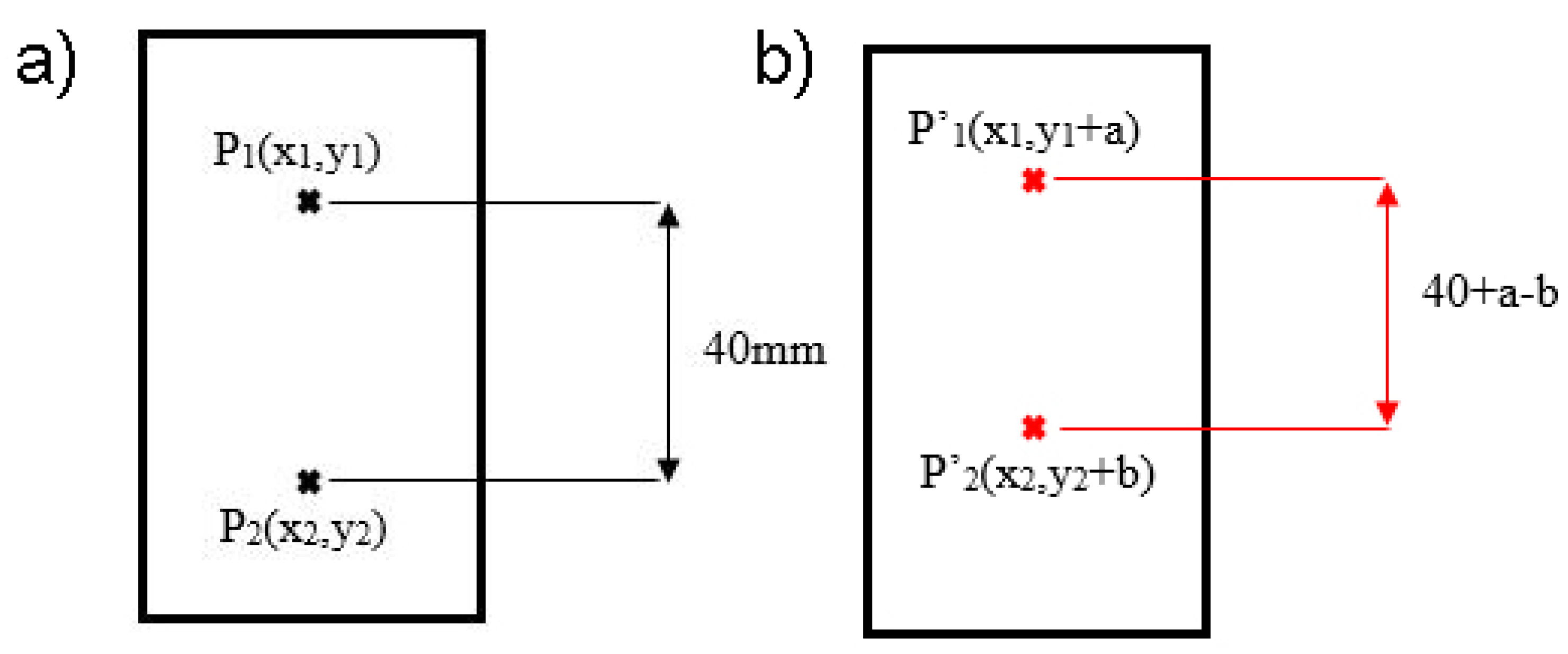
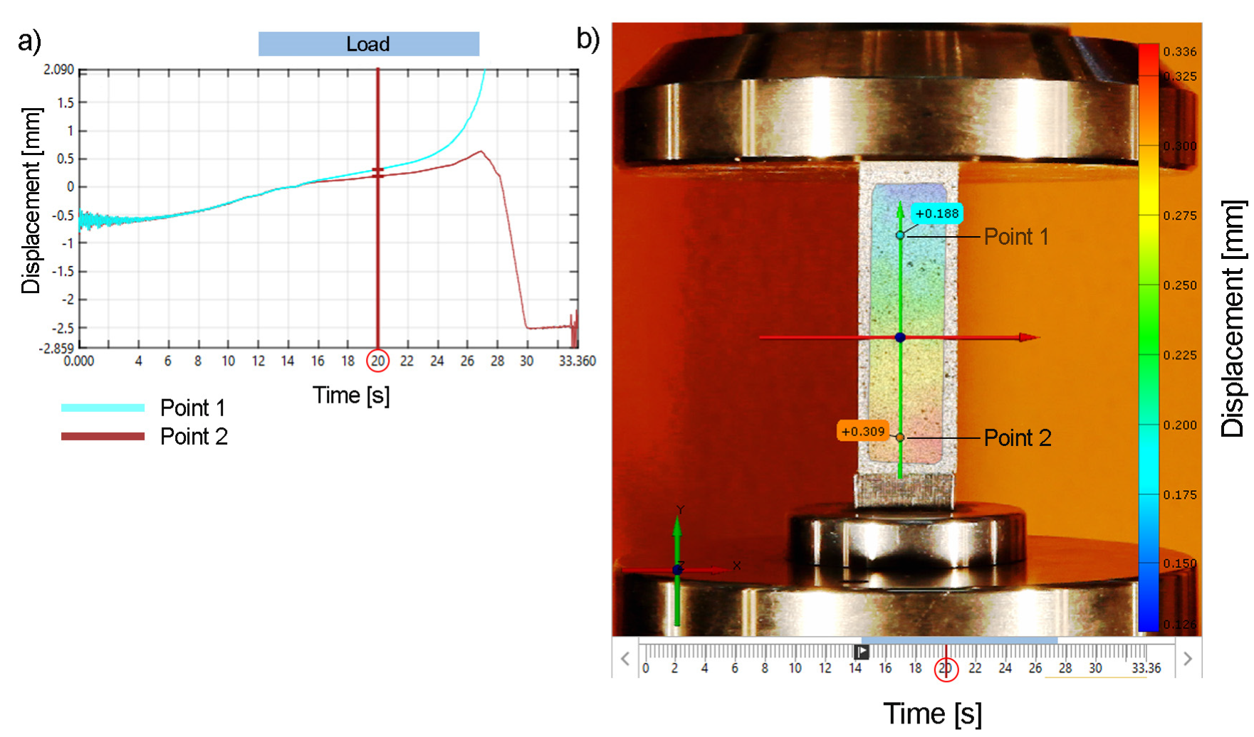
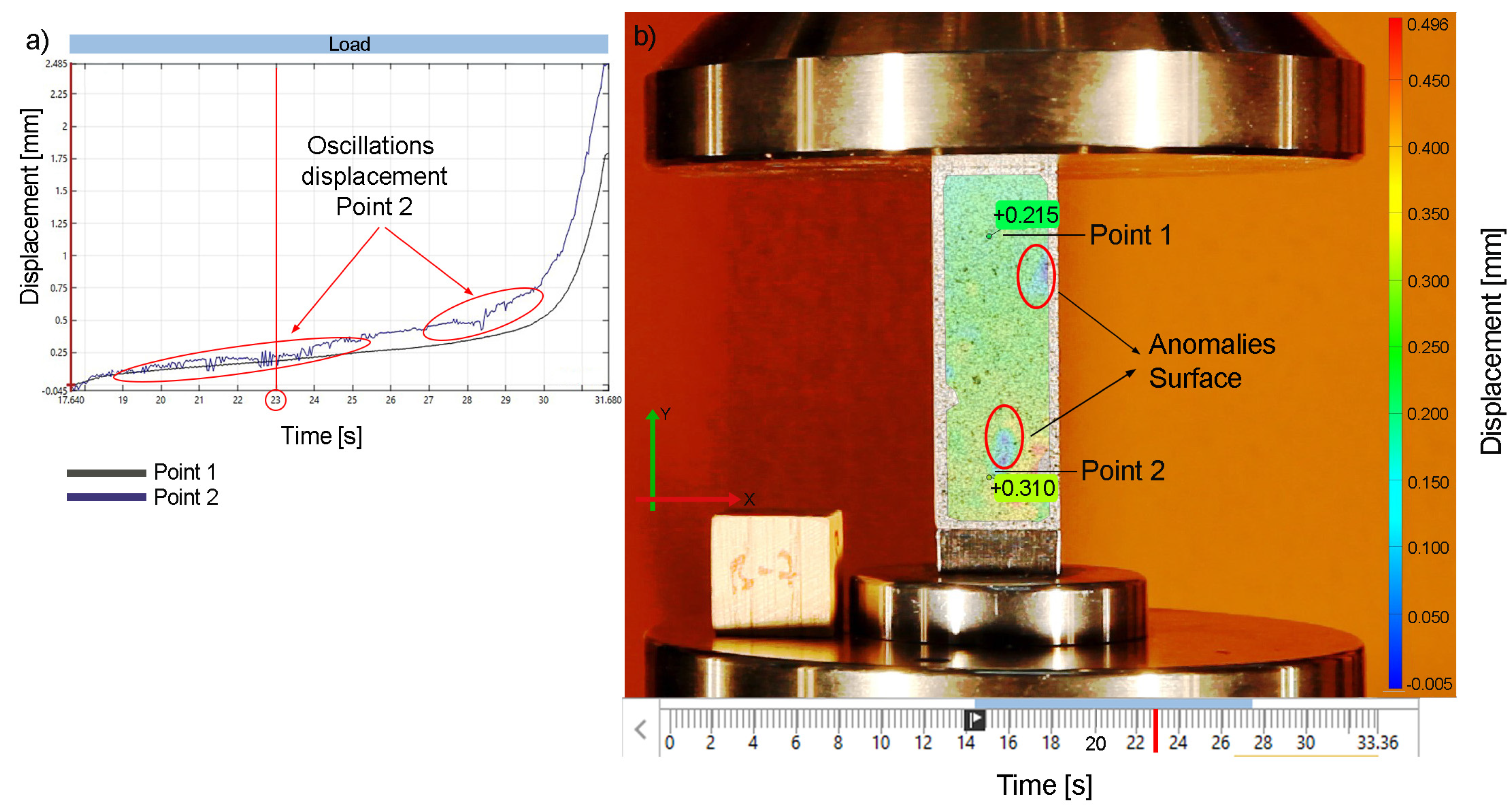
2.3. Displacement Analysis

When all samples were tested and recorded, all frames were entered into the GOM Correlate software and the reference image was defined. The next step was the analysis using DIC. Although DIC is an internal process carried out by the software, it is necessary to previously enter a series of initial parameters, which are detailed below.

First, the study surface (referred to as the “surface component” in the software) is defined for which the DIC is to be conducted. The quality of the pattern is quantified using a color map (in this case green). To avoid possible distortions in the contours, it is necessary to define an analysis surface that does not exceed the limits of the pattern and is inside the surface of the specimen.

The next step is to set the coordinate axis to adjust the orientation of the specimen to the direction in which the displacements will be measured. However, for the recording of the tests, a tripod with a level was used and the focus cross was stabilized to establish the horizontal axis of the specimen, thus, in most cases the adjustment of the coordinate axis was not required. It was sufficient to place the vertical axis, “y”, which was positive in the up direction, on the edge of the specimen to guarantee verticality. Perpendicular to this was the “x” axis, which was positive to the right.

Following the definition of the initial parameters, the displacement calculation was carried out. A color map was obtained with a scale on the side that indicates the length (mm) of the displacements of each of the points (Figure 4). Thus, the surface was defined allowing the displacement to be obtained at any point.

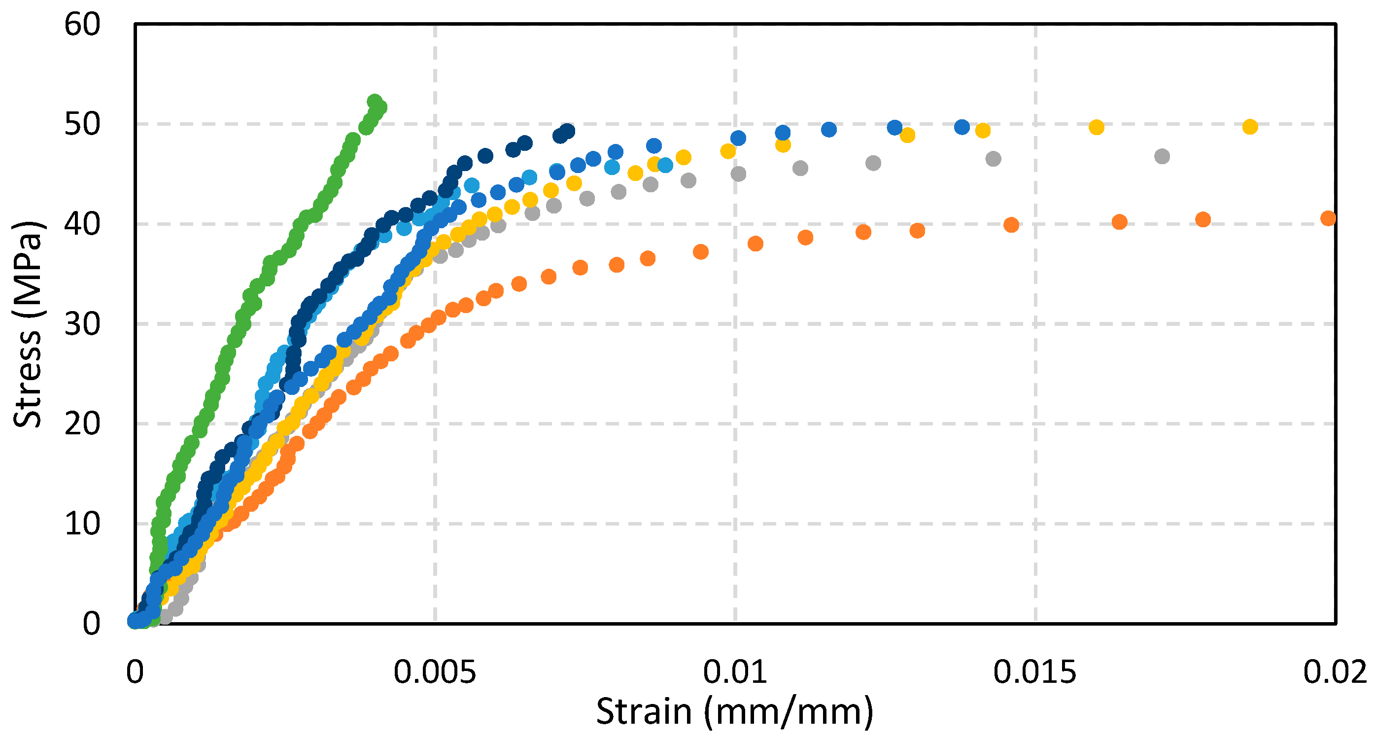
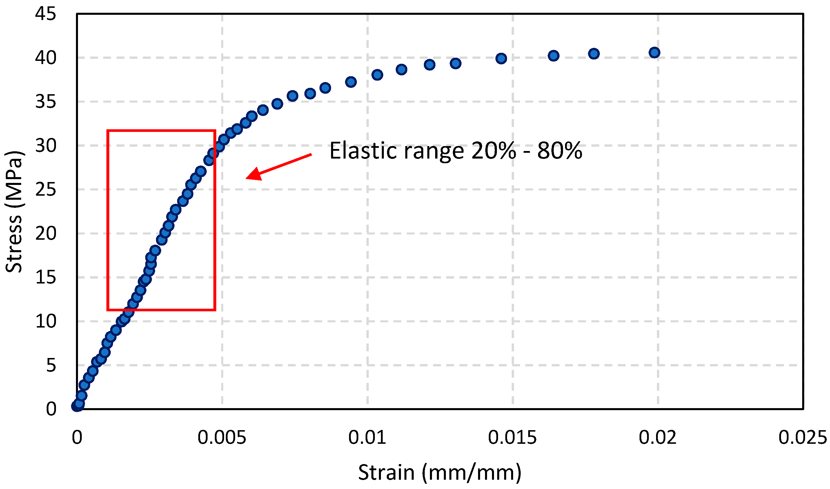
2.4. Strain’s Calculation

After obtaining the displacement in each of the frames, it was necessary to calculate the strain experienced by the specimen. The UNE standard: 56535: 1977 (updated 2017) [10] establishes that the measurement of strain must be carried out at the center of the test piece because the contours will suffer greater strain (due to crushing by direct contact with the load of the plates). For this reason, a virtual extensometer was placed, using two centered and separated points from these contours to avoid these distortions.

First, two points were defined in the initial reference image of the test whose coordinates were P₁ (x₁, y₁) and P₂ (x₂, y₂) (Figure 5a), and their initial separation was 40 mm.

When the load is first applied, the specimen deforms and consequently these points will change position. The displacement of the lower points will be greater than that of the upper points because the load is applied by lifting the lower plate. Therefore, the position of these points will vary in the manner shown in Figure 5b, allowing the unit deformation in each of the frames corresponding to the different moments of the test to be obtained with Equation (7).

$$\epsilon =\frac{b-a}{40}$$

(7)

Figure 6 shows the displacement/time diagram of test piece A1 as a result of the software, in which the evolution of the displacements over time in the load section is shown for points 1 and 2. These values were exported to a spreadsheet.

Finally, the load and strain data were synchronized, and a recording frequency allowed the association of a frame with strain and stress values every 0.2 s.

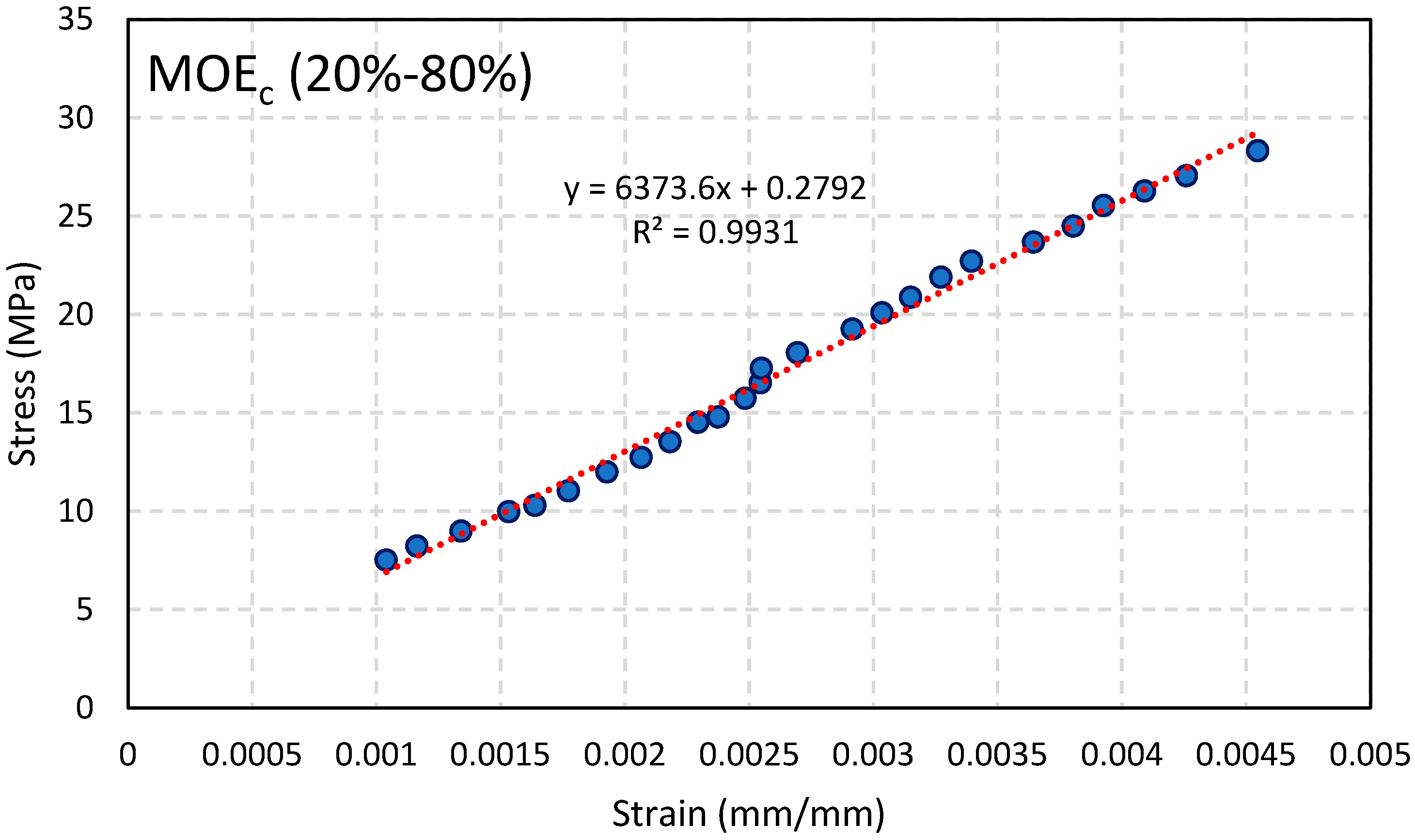
2.5. Obtaining the MOE_c and MOR_c

Following the relation of the corresponding strains to the load data, the necessary means are already available to obtain the MOE_c, which is equivalent to the slope of the line that constitutes the elastic zone in the stress/strain graph.

The behavior of wood usually passes through three different phases [51]: (a) the elastic zone; (b) the so-called elasto-plastic zone; and (c) the plastic or creep zone. Figure 7 shows stress/strain curves corresponding to the samples of Series A.

However, the specimen may also present imperfections, both geometric (due to the cutting process) and specific to the material (pores, internal cracks, knots, etc.). In these cases, the load distribution in the first moments may not be uniform, causing distortions in the initial outline of the curve until the load distribution is regularized. These loads generally represent 10% to 15% of the load that defines the elastic limit. Therefore, in practice, the initial point of the line that determines the modulus of elasticity (MOE_c) begins to be measured from the value that corresponds to 20% of the elastic limit stress [52].

The elastic limit is the theoretical point at which the elastic zone ends. However, it is difficult to determine this limit exactly because the change in slope between the elastic and elasto-plastic zone is very subtle. Furthermore, measurements can be distorted depending on the mode of failure and where it occurs. In these cases, the end point of the line that determines the MOE_c is taken as the value corresponding to 80% of the elastic limit. This can be seen in Figure 7, which shows that some samples do not follow the general trend.

Figure 8 and Figure 9 show the process for obtaining the MOE_c in the plotting of the curve for sample A1.

The maximum strength to compression parallel to the fibers (MOR_c) is obtained by means of the relationship between the maximum load that the specimen is capable of supporting before its breakage, and its surface. This value can be obtained directly from the testing machine.

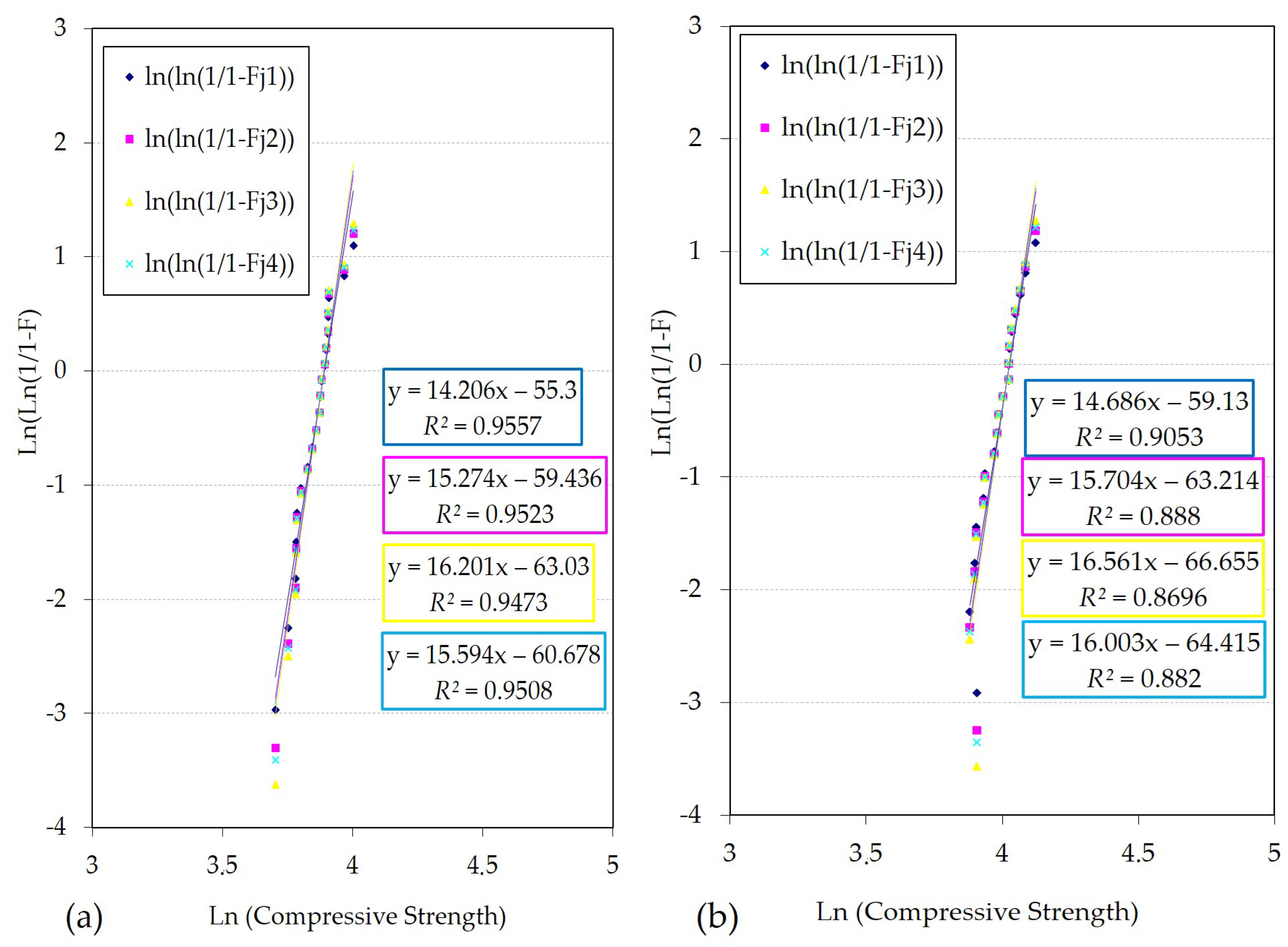
2.6. Assessment of Reliability Using the Weibull Modulus Based on Compression Strength Data

The Weibull distribution is an important tool for studying the reliability of materials, because they can exhibit significant variability in their characteristics and present premature failures. The Weibull distribution is flexible and adaptable to a wide range of data [53,54] Furthermore, the two-parameter Weibull distribution has a simple equation (type y = a x + b) and the coefficients can be easily estimated from experimental data and with the help of failure estimators (Fj). The slope of the line is defined as the Weibull modulus and represents the reliability of the material with respect to a key property. In the present work, four most common estimators in the literature were used [46,55,56]:

$$\mathrm{Fj}1=\frac{\mathrm{j}}{\left(\mathrm{n}+1\right)}$$

(8)

$$\mathrm{Fj}2=\frac{\mathrm{j}-0.3}{\left(\mathrm{n}+0.4\right)}$$

(9)

$$\mathrm{Fj}3=\frac{\mathrm{j}-0.5}{\mathrm{n}}$$

(10)

$$\mathrm{Fj}4=\frac{\mathrm{j}-\frac{3}{8}}{\left(\mathrm{n}+1/4\right)}$$

(11)

To interpret the results obtained by the line, the value of the slope (Weibull’s modulus) and the correlation coefficient R² were used, whose value varies between 0 and 1, and indicates the degree of correlation between the studied data.

A higher Weibull modulus (greater slope of the line) indicates a more reliable material, that is, it has a lower dispersion and the population has a narrower distribution. Conversely, if the Weibull modulus is low, it means that there is little reproducibility of values and a wide range of variation, as in ceramic materials [57].

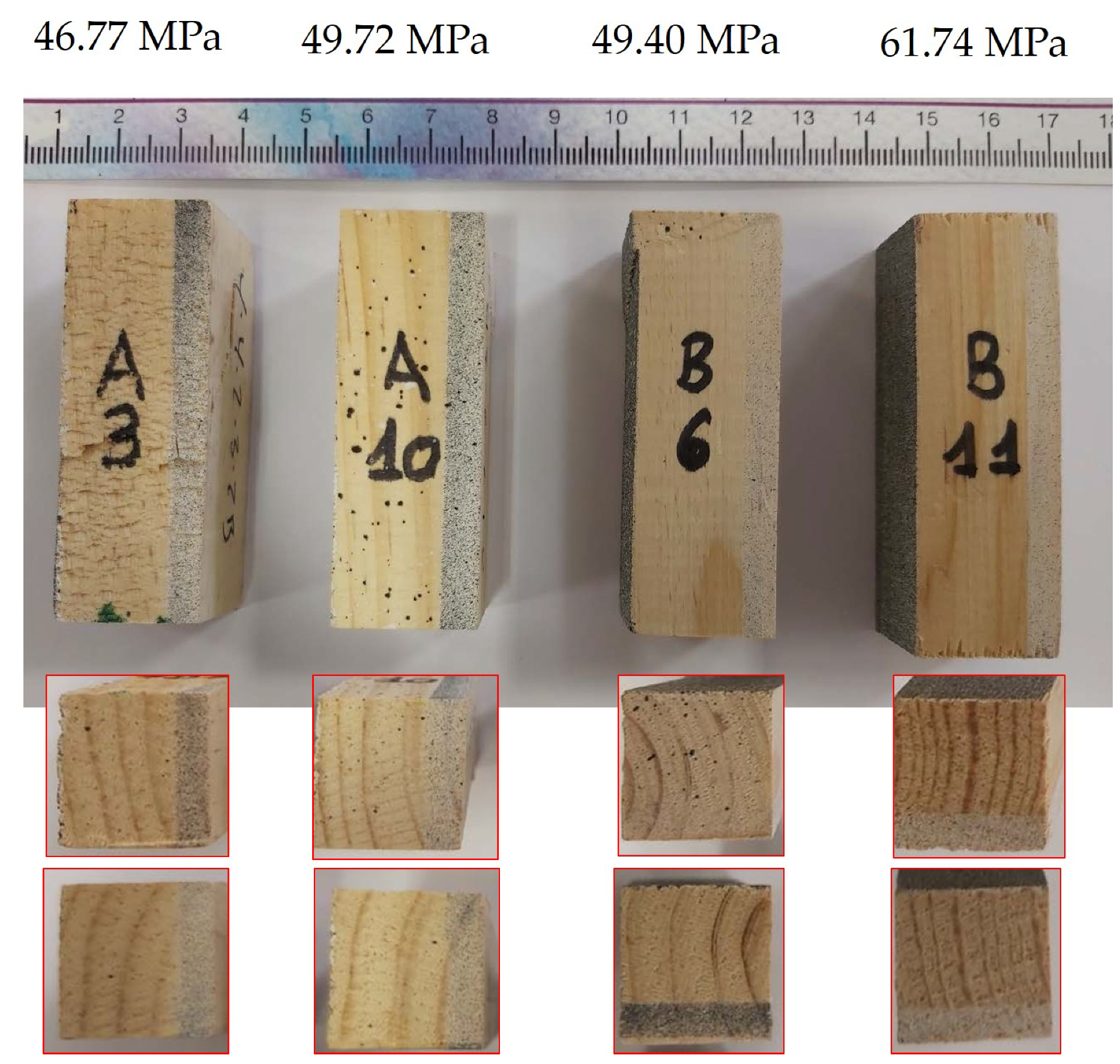
2.7. Macroscopic and Microscopic Study

As a complement to the strength and reliability data, a brief micro and macrostructural study was carried out on some of the samples selected for traceability. For this examination, a ZEISS Axiovert 100 A microscope (Jena, Germany) was used to observe the samples’ surface condition. The microscope has a 3 MP Optika (Ponteranica, Italy) digital camera controlled by Optika Vision Lite software. A Handheld Digital Pro 5 MP microscope-magnifying glass from Celestron (Torrance, CA, USA) equipped with a white LED-type light was also used to take macrographs of the test tubes. In addition, the average ring width was measured by the free software ImageJ^® [58] using a Handheld Digital Pro 5 MP microscope.

3. Results and Discussion

Table 3. Average value of compressive strength (MOR_c) and MOE_c, density, and ring width.

	Parallel Compression of Fibers
	Samples	MORc (MPa)	MOEc (MPa)	Standard Deviation MORc (MPa)	Standard Deviation MOEc (MPa)
Average A	19	47.39	9072	3.53	2304
Average B	18	54.23	10,348	3.80	1940
Total Average	37	50.72	9693	5.00	2202
	Samples	Density (kg/m3)	Standard Deviation density (kg/m3)	Ring width (mm)	Standard Deviation ring width (mm)
Average A	19	561	33	3.04	0.61
Average B	18	597	34	2.93	1.30
Total Average	37	579	38	2.99	1.00

shows the mean values and their respective deviations for the specimens from both trees and the total of the tests and samples carried out. The variables to be analyzed in all of them are the maximum strength (MPa) and the modulus of elasticity (MPa).

As shown, the average values of MOR_c and MOE_c for both series show an appreciable difference, although the standard deviation is sufficient to see that both series overlap for both of the properties evaluated. Series B shows higher compressive strength and modulus of elasticity than Series A. By plotting the frequency histogram (Figure 10), the location of samples from both series can be approximately detected. Each series separately has a normal behavior and together they also generate a normal curve with overlap. The distributions corresponding to MOE_c, density, and ring width also fit normal distributions, although the separation of the two series is not clear.

The average density of Series A shows a lower value than that of Series B, and the two series present the same standard deviation. The average ring width is similar for both series, although the standard deviation for Series B shows a greater deviation. This is because the samples are mostly from the sapwood and the heartwood, with fewer specimens from the middle zone. However, Series A shows representatives from all zones. The selection of specimens was random, so it was not necessary to equally represent all areas of the trunk. Nonetheless, the average values of the ring width were similar.

Table 4. Summary of the linear regression and quadratic adjustment.

	MORc (MPa)		MOEc (MPa)
Total (37 samples)	Linear regression	R²	Linear regression	R2
Density (kg/m3)	y = 0.0972x − 5.5492	0.541	y = 16.582x + 95.762	0.0812
Ring width (mm)	y = −2.1901x + 57.101	0.1585	y = −879.66x + 12,256	0.1319

shows the summary of the linear regression and quadratic adjustment (R²) of the two physical variables (density and ring width) on the mechanical variables (MOR_c and MOE_c). Density has a direct influence on MOR_c, whereas the ring width does not have a clear influence, although it appears that a smaller ring width (sapwood) leads to greater compressive strength. The influence on the MOE_c is not clearly defined for either of the two physical characteristics. All R² values are poor, however, R² between MOR_c and density is acceptable.

The MOR_c values are close to the theoretical values that appear in the literature: 45.4 MPa according to [59] and 47.6 MPa according to [60], which are within the 45–62 MPa interval proposed by [61]. Thus, it can be determined that the values obtained in the conducted tests are valid by attributing the existing difference to the variability that can be found within the species.

The MOE_c value is below all of the theoretical values that appear in the literature: 9950 MPa according to [59], 10,873 MPa according to [60], and 10,600–14,500 MPa according to [61]. However, it must be taken into account that these values correspond to the results of MOE_f bending tests, so the MOEc value must be lower than these [16]. Thus, it can be verified that the values obtained for this property are valid because they are below the bending values but close to them. Finally, the average value of the density remains within the interval reported by [5,6].

It should be noted that some specimens (A4, B3, and B7) were discarded (of the initial 20 of each series) for the calculation of the final parameters because they presented a low R² value in the linear regression used to estimate the modulus of elasticity (MOE_c), in addition to erratic behavior, and slippage of the specimens occurred during the test, leading to errors in the measurement of compressive strength.

Figure 11 and Figure 12 show the tests of two of the failed specimens, in which, due to the dotted texture, the anomalous areas that led to premature failure are clearly detected, even before their breakage. Thus, DIC is shown to be a sensitive and low-cost technique, compared to others, which directly and visually allows detection of faults and anomalous areas in the tested specimens.

An example is found in the case of test piece B3. In Figure 11a, point P₂ shows oscillations in its displacement throughout the loading process. In the diagram, the red line (corresponding to the evolution of the displacements of the lower point P₂) undergoes large oscillations in certain sections, such as the intervals from 24 to 27 s and from 40 to 42 s. If the displacement map of the test piece is analyzed (Figure 11b), it is observed that the surface has certain areas in which the displacements are lower. This indicates the existence of defects or anomalies in the lower part of the specimen (coinciding with the final breakage of the specimen that occurs in the lower zone).

Another case is the specimen B7. In the diagram of Figure 12a, the blue line (corresponding to the evolution of the displacements of the lower point P₂) undergoes large oscillations, mainly from the beginning to 26 s and in the interval from 28 to 29 s. However, the black line (corresponding to the evolution of the displacements of the upper point P₁) appears to be regular. If the displacement map of specimen B7 is analyzed (Figure 12b), the surface presents certain areas in which the displacements are lower, as in the previous case. This indicates the existence of defects or anomalies in the lower part of the specimen.

3.1. Determination of Reliability

Wood is a widely used material that can experience random breaks and failures. Due to its natural variability, it is feasible to apply the Weibull distribution to determine its reliability and therefore its behavior in service. The Weibull graphs are plotted from the compression tests carried out on the wood specimens of both series (A and B). Because there were sufficient tests to carry out an acceptable reliability study on each series (A and B), their Weibull modules were determined as a measure of reliability in each tree (Figure 13).

As can be seen, the Weibull modulus is similar for both series with very close values for the best estimator Fj3 (Equation (10)), although the quadratic R² fits are less than or equal to 0.90 for Series B, whereas for Series A they are greater than 0.95. Series B shows a Weibull modulus for the third estimator that is somewhat higher (16.561) but with a poor fit. A Weibull modulus of 16 (Fj3) for each tree (or series) can be considered acceptable and, within the same tree, the reliability is good. The estimator with the best regression is Fj1 (Equation (8)), which has a value of around 14 for both series. It can be concluded that the reliability of this type of wood is in the interval between 14 and 16. Although few studies exist on the reliability of wood using its compressive strength as a key property, by way of comparison this behavior is higher than that described in [62].

After it was determined that the reliability of both series remained at very close values, the distribution was applied to all of the correct tests (37), because the same material was being tested: there was no difference in terms of the conditions of the materials’ growth because they were collected in the same geographical area and their size was similar.

In addition, four specimens (two of each of the series) were randomly taken with their individual values of compressive strength (Figure 14) to determine the traceability of the samples with the data represented in the graph (Figure 15) and perform a complementary microstructural study (Figure 16, Figure 17, Figure 18, Figure 19, Figure 20, Figure 21 and Figure 22). Specimens were selected in the high, medium, and low resistance ranges.

As can be seen when joining the data from both series, a Weibull modulus was obtained that is lower than that obtained for each series separately, as expected. However, the value of 12.362 with an R² value of 0.944 is not significantly lower than that previously calculated. If the higher value of R² is taken, the Weibull modulus drops slightly, reaching 11.380. In this case, the value of the slope or Weibull modulus is between 11 and 12 for this type of wood. This is the most appropriate value for the global reliability of the wood because, with regard to its structural use, there is no discrimination between different trees, which had a similar quality.

From the data provided by the Weibull lines for the different estimators, the characteristic strength of this type of wood can be deduced for both series, that is, the set of data. The results of the regression line, quadratic fit, characteristic strength, and Weibull modulus as a measure of reliability are shown in

Table 5. Values obtained from the Weibull distribution.

Linear Regression	R2	Characteristic Strength (MORc)	Weibull Modulus
y = 11.380 x − 45.169	0.9578	52.94	11.380
y = 11.915 x − 47.283	0.9514	52.90	11.915
y = 12.362 x − 49.047	0.9440	52.85	12.362
y = 12.072 x − 47.900	0.9490	52.87	12.072

.

It can be verified that the result obtained for characteristic strength is slightly higher than the previously determined average value, but is within the range indicated by the literature.

The application of the Weibull distribution using the MOE_c as a key property is different from the values obtained for strength (MOR_c), mainly due to the way this property is determined from the test curve, and results in a value of the Weibull modulus of around 6. Its adaptation to the regression line is around 0.87 and 0.88.

It can be concluded that the Weibull distribution is applicable to the strength values of this type of wood (MOR_c), but less so to the MOE_c values. Thus, the most suitable key property for determining material reliability is MOR_c.

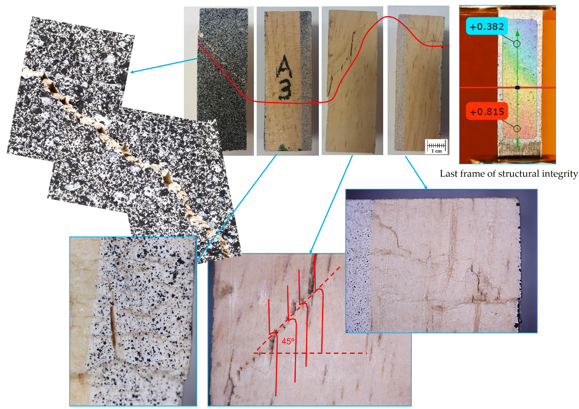
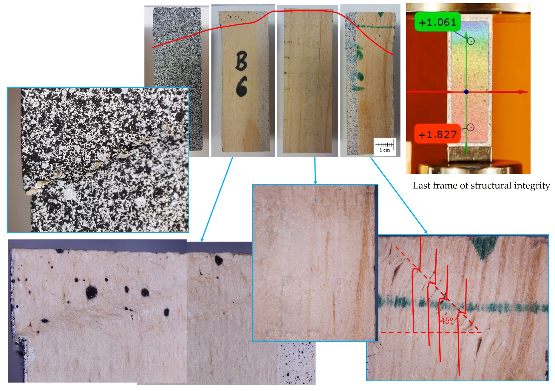
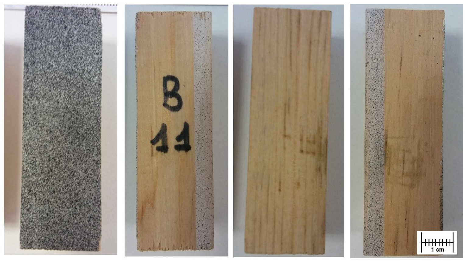
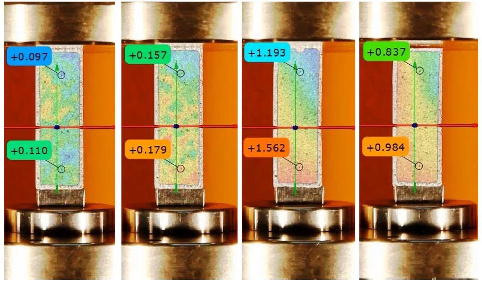
3.2. Macroscopic and Microscopic Study

As a complement to the strength and reliability study, a microstructural study was carried out on some samples (Figure 16, Figure 17, Figure 18, Figure 19, Figure 20, Figure 21 and Figure 22), specifically those that were chosen to evaluate the traceability of the Weibull regression. Figure 15 shows the macroscopic appearance of the samples. An example of the surface finish of the specimens is shown in Figure 16a. Figure 16b, in which the fibers can be observed, shows the upper face of the specimens.

Figure 17 and Figure 18 show microstructural details of the wood. Figure 16a shows the presence of heterogeneities with the associated porosity. If this type of defect is large, it can reduce the mechanical properties. These defects can remain on the surface, be very small, and have little impact on the strength of the specimen. In contrast, if they remain inside the specimen and are large, they can cause premature failure, without prior notice. Figure 18 shows the type of staggered breakage (at 45°) of the fibers of the material on the face corresponding to the speckled texture.

Figure 19, Figure 20, Figure 21 and Figure 22 show the macrographic studies of the four control specimens (A3, A10, B6, and B11) of both trees, in comparison with the last frame of structural integrity. In the specimens A3, A10, and B6, the typical 45° breakage of the wood is observed. Whereas in A3 (Figure 19) the break occurred in the middle of the piece, in both A10 and B6 it was located in the upper portion. Specimen A3 shows the least resistance, but also underwent a central break at 45°, as shown by the last frame of the piece with structural integrity (without break). Specimens A10 (Figure 20) and B6 (Figure 21) show similar values in terms of compressive strength parallel to the fibers. The macrographic study fully coincides with the resistant behavior offered by the samples: the breaks were similar and both broke in the upper area at 45° angles but with less clarity than in the first case. The last frame shows the upper break, in addition to a mixture of the breaks of the four faces. There was no apparent breakage of the specimen B11 (Figure 22), although it underwent crushing, because this specimen was selected from the sapwood area of the trunk, which presents higher compressive strengths than the middle and heartwood areas (A3, A10, and B6) [47]. Each case is compared with the last frame in which there was integrity in the specimen, i.e., it maintained its shape without breaking. It can be seen how the use of the DIC roughly predicts the break zone a few milliseconds before the sample breaks. In the case of the test piece B11, the forces are distributed along the length of the test piece and, at the end, it recovers, maintaining its parallelepiped shape.

4. Conclusions

Digital Image Correlation is presented as an appropriate technique for the study of wood strain mainly due to its precision, low cost, and non-invasive and non-destructive nature. As such, it is an ideal alternative to other more conventional techniques, such as strain gauges, that suffer from these problems.

In this article, a methodology for obtaining the mechanical properties of wood was proposed, developed, and tested, based on compression testing and Digital Image Correlation (DIC). The axial compression tests were synchronized using DIC so that the loads applied at each moment were related to the strain caused by the loads. As a consequence, the proposed implementation of the DIC technique, in combination with compression testing, was achieved.

The treatment of data resulting from the tests (strain and load applied over time) made it possible to determine the mechanical properties of the Pinus halepensis Mill. species. Average values of MOR_c of 50.6 MPa and MOE_c of 9670 MPa were obtained.

Density has a direct influence on MOR_c, whereas the ring width does not have a clear influence. The influence on the MOE_c is not clearly defined for either of the two physical characteristics.

A total of 37 two-tree specimens (Series A and B) were tested and statistical analysis was conducted using the Weibull distribution. It was shown that this type of wood is adequately adapted to this type of distribution. Reliability values of the Weibull modulus of 14 to 16 were obtained for each of the series for the four estimators studied, whereas the mean value of the reliability of the material was in the interval between 11 and 12 for the four estimators.

The value of the characteristic resistance calculated from the Weibull distribution was also determined, and lay in a range between 52 and 53 MPa.

The most suitable key property for determining reliability is the MOR_c for these types of materials. However, the use of the MOE_c was shown to be unsuitable.

Finally, it was shown that there was consistency between the microstructural study after failure and the DIC results of the specimens during the test. A relationship was found between the last frame readings with structural integrity (pre-break) and the break-after-failure analysis. This indicates that DIC can predict the type of specimen failure milliseconds before structural failure. Therefore, DIC was found to be an inexpensive and non-invasive technique to predict structural failure of this type of material.

References

1. Saavedra Flores, E.I.; Dayyani, I.; Ajaj, R.M.; Castro-Triguero, R.; DiazDelao, F.A.; Das, R.; González Soto, P. Analysis of cross-laminated timber by computational homogenisation and experimental validation. Compos. Struct. 2015, 121, 386–394. [Google Scholar] [CrossRef]
2. Morland, C.; Schier, F.; Janzen, N.; Weimar, H. Supply and demand functions for global wood markets: Specification and plausibility testing of econometric models within the global forest sector. For. Policy Econ. 2018, 92, 92–105. [Google Scholar] [CrossRef]
3. Jonsson, R.; Rinaldi, F. The impact on global wood-product markets of increasing consumption of wood pellets within the European Union. Energy 2017, 133, 864–878. [Google Scholar] [CrossRef]
4. Falk, R.H. Robert Wood as a Sustainable Building Material. J. For. Prod. 2009, 59, 6–12. [Google Scholar]
5. Correal-Mòdol, E.; Vilches Casals, M. Properties of clear wood and structural timber of Pinus halepensis from north-eastern Spain. In Proceedings of the World Conference on Timber Engineering (WCTE), Auckland, New Zealand, 15–19 July 2012. [Google Scholar]
6. Elaieb, M.T.; Shel, F.; Elouellani, S.; Janah, T.; Rahouti, M.; Thévenon, M.F.; Candelier, K. Physical, mechanical and natural durability properties of wood from reforestation Pinus halepensis Mill. in the Mediterranean Basin. Bois For. Trop. 2017, 1, 19–31. [Google Scholar] [CrossRef]
7. Quinteros-Mayne, R.; de Arteaga, I.; Goñi-Lasheras, R.; Villarino, A.; Villarino, J.I. The influence of the elastic modulus on the finite element structural analysis of masonry arches. Constr. Build. Mater. 2019, 221, 614–626. [Google Scholar] [CrossRef]
8. Cáceres Hidalgo, E. Caracterización Físico-Mecánica de la Madera de Paulownia Elongata; Universidad de Valladolid: Valladolid, Spain, 2016. [Google Scholar]
9. European Standard. EN 1995-1-1 (2004): Eurocode 5: Design of Timberstructures-Part 1-1: General-Common Rules and Rules Forbuildings; European Committee of Standardization (CEN): Brussels, Belgium, 2004; p. 123. [Google Scholar]
10. Spanish Standard. UNE 56535:1977 Características Físico-Mecánicas de la Madera; Asociación Española de Normalización (AENOR): Madrid, Spain, 2011. [Google Scholar]
11. European Standard. EN 408+A1:2012. Timber Structures. Structural Timber and Glued Laminated Timber. Determination of Some Physical and Mechanical Properties; European Committee of Standardization (CEN): Brussels, Belgium, 2012. [Google Scholar]
12. C, I.D.E.A.; Antonio, J.; Ordóñez, B.; Masera, O. Madera y Bosques. 2001. Available online: https://myb.ojs.inecol.mx/index.php/myb (accessed on 28 October 2020).
13. Nogueira, M.; Ballarin, A.W. Sensibilidade dos ensaios de ultra-som à ortotropia elástica da madeira. In Proceedings of the Conferência Pan-Americana de Ensaios Não-Destrutivos, Salvador, Brazil, 25 May 2003; p. 3. [Google Scholar]
14. Esteban, L.G.; de Palacios, P.; García Fernández, F.; García-Iruela, A.; del Pozo, J.C.; Pérez Borrego, V.; Agulló Pérez, J.; Padrón Cedrés, E.; Arriaga, F. Characterisation of Pinus canariensis C.Sm. ex DC. Sawn Timber from Reforested Trees on the Island of Tenerife, Spain. Forests 2020, 11, 769. [Google Scholar] [CrossRef]
15. Šilinskas, B.; Varnagiryte-Kabašinskiene, I.; Aleinikovas, M.; Beniušiene, L.; Aleinikoviene, J.; Škema, M. Scots pine and norway spruce wood properties at sites with different stand densities. Forests 2020, 11, 587. [Google Scholar] [CrossRef]
16. Argüelles Álvarez, F.R.; Arriaga Martitegui, M.; Esteban Herrero, G.Í.; González, R.A.B. Estructuras de Madera Bases de Cálculo; AITIM: Madrid, Spain, 2013. [Google Scholar]
17. Baño, V.; Cetrangolo, G.; Morquio Hugo O’Neill, A. Stress-strain diagram of free-defects timber of pinus elliottii from Uruguay. In Proceedings of the XXXVI Jornadas Sudamericanas de Ingeniería Estructural, Montevideo, Uruguay, 19–21 November 2014. [Google Scholar]
18. Moya, L.; Baño, V. Elastic behavior of fast-growth Uruguayan pine determined from compression and bending tests. BioRes 2017, 12, 5896–5912. [Google Scholar] [CrossRef] [Green Version]
19. Bucur, V. Acoustic of Wood. In Acoustics of Wood; Springer: Berlin/Heidelberg, Germany, 2006; pp. 1–4. ISBN 978-3-540-26123-0. [Google Scholar]
20. Álvaro Pérez Ortega Comparación de Ensayos a Compresión de Madera Estructural Mediante Norma UNE y Norma ASTM; Universidad de Valladolid: Valladolid, Spain, 2014.
21. Sutton, M.; Orteu, J.; Schreier, H. Image Correlation for Shape, Motion and Deformation Measurements: Basic Concepts, Theory and Applications; Springer Science & Business Media: Berlin/Heidelberg, Germany, 2009. [Google Scholar]
22. Pan, B.; Qian, K.; Xie, H.; Asundi, A. Two-dimensional digital image correlation for in-plane displacement and strain measurement: A review. Meas. Sci. Technol. 2009, 20, 062001. [Google Scholar] [CrossRef]
23. Allaoui, S.; Rekik, A.; Gasser, A.; Blond, E.; Andreev, K. Digital Image Correlation measurements of mortarless joint closure in refractory masonries. Constr. Build. Mater. 2018, 162, 334–344. [Google Scholar] [CrossRef]
24. Sánchez-Aparicio, L.J.; Villarino, A.; García-Gago, J.; González-Aguilera, D. Photogrammetric, geometrical, and numerical strategies to evaluate initial and scurrent conditions in historical constructions: A test case in the church of San Lorenzo (Zamora, Spain). Remote Sens. 2016, 8, 60. [Google Scholar] [CrossRef] [Green Version]
25. García-Martin, R.; López-Rebollo, J.; Sánchez-Aparicio, L.J.; Fueyo, J.G.; Pisonero, J.; González-Aguilera, D. Digital image correlation and reliability-based methods for the design and repair of pressure pipes through composite solutions. Constr. Build. Mater. 2020, 248, 118625. [Google Scholar] [CrossRef]
26. Fayyad, T.M.; Lees, J.M. Application of Digital Image Correlation to Reinforced Concrete Fracture. Procedia Mater. Sci. 2014, 3, 1585–1590. [Google Scholar] [CrossRef] [Green Version]
27. Aghlara, R.; Tahir, M.M. Measurement of strain on concrete using an ordinary digital camera. Meas. J. Int. Meas. Confed. 2018, 126, 398–404. [Google Scholar] [CrossRef]
28. Krishnan, S.A.; Moitra, A.; Sasikala, G.; Baranwal, A.; Moitra, A.; Sasikala, G.; Albert, S.K.; Bhaduri, A.K.; Harmain, G.A.; Jayakumar, T.; et al. Assessment of Deformation Field during High Strain Rate Tensile Tests of RAFM Steel Using DIC Technique. Procedia Eng. 2014, 86, 131–138. [Google Scholar] [CrossRef] [Green Version]
29. Guo, N.; Liang, J.; Yu, Q.; Qian, B. Plastic evolution behavior of H340LAD_Z steel by an optical method. Phys. B Condens. Matter 2017, 506, 69–74. [Google Scholar] [CrossRef]
30. López-Alba, E.; López-García, R.; Dorado, R.; Díaz, F.A. Aplicación de correlación digital de imágenes para el análisis de problemas de contacto. In Proceedings of the XIX Congreso Nacional de Ingeniería Mecánica, Castellón de la Plana, Spain, 15–16 November 2012; p. 8. [Google Scholar]
31. Pablo Canal Casado, L. Experimental and Computational Micromechanical Study of Fiber-Reinforced Polymers; Universidad Politécnica de Madrid: Madrid, Spain, 2011. [Google Scholar]
32. Sabato, A.; Niezrecki, C. Feasibility of digital image correlation for railroad tie inspection and ballast support assessment. Meas. J. Int. Meas. Confed. 2017, 103, 93–105. [Google Scholar] [CrossRef]
33. Zink, A.G.; Hanna, R.B.; Stelmokas, J.W. Measurement of Poisson’s ratios for yellow-poplar. For. Prod. J. 1997, 47, 78–80. [Google Scholar]
34. Bjurhager, I.; Berglund, L.A.; Bardage, S.L.; Sundberg, B. Mechanical characterization of juvenile European aspen (Populus tremula) and hybrid aspen (Populus tremula × Populus tremuloides) using full-field strain measurements. J. Wood Sci. 2008, 54, 349–355. [Google Scholar] [CrossRef]
35. Jeong, G.Y.; Hindman, D.P.; Zink-Sharp, A. Orthotropic properties of loblolly pine (Pinus taeda) strands. J. Mater. Sci. 2010, 45, 5820–5830. [Google Scholar] [CrossRef]
36. Jeong, G.Y.; Park, M.J. Evaluate orthotropic properties of wood using digital image correlation. Constr. Build. Mater. 2016, 113, 864–869. [Google Scholar] [CrossRef]
37. Guindos, P.; Ortiz, J. The utility of low-cost photogrammetry for stiffness analysis and finite-element validation of wood with knots in bending. Biosyst. Eng. 2013, 114, 86–96. [Google Scholar] [CrossRef]
38. Kunecký, J.; Sebera, V.; Hasníková, H.; Arciszewska-Kędzior, A.; Tippner, J.; Kloiber, M. Experimental assessment of a full-scale lap scarf timber joint accompanied by a finite element analysis and digital image correlation. Constr. Build. Mater. 2015, 76, 24–33. [Google Scholar] [CrossRef]
39. Méité, M.; Dubois, F.; Pop, O.; Absi, J. Mixed mode fracture properties characterization for wood by Digital Images Correlation and Finite Element Method coupling. Eng. Fract. Mech. 2013, 105, 86–100. [Google Scholar] [CrossRef]
40. Ritschel, F.; Zhou, Y.; Brunner, A.J.; Fillbrandt, T.; Niemz, P. Acoustic emission analysis of industrial plywood materials exposed to destructive tensile load. Wood Sci. Technol. 2014, 48, 611–631. [Google Scholar] [CrossRef] [Green Version]
41. Jeong, G.Y.; Zink-Sharp, A.; Hindman, D.P. Applying digital image correlation to wood strands: Influence of loading rate and specimen thickness. Holzforschung 2010, 64, 729–734. [Google Scholar] [CrossRef]
42. Liu, J.Y. A weibull analysis of wood member bending strength. J. Mech. Des. Trans. ASME 1982, 104, 572–577. [Google Scholar] [CrossRef]
43. Zhong, Y.; Wu, G.; Ren, H.; Jiang, Z. A determination method of compressive design value of dimensional lumber. J. Wood Sci. 2018, 64, 526–537. [Google Scholar] [CrossRef] [Green Version]
44. Owens, F.C.; Verrill, S.P.; Shmulsky, R.; Kretschmann, D.E. Distributions of moe and mor in a full lumber population. Wood Fiber Sci. 2018, 50, 265–279. [Google Scholar] [CrossRef] [Green Version]
45. Ono, K. A simple estimation method of Weibull modulus and verification with strength data. Appl. Sci. 2019, 9, 1575. [Google Scholar] [CrossRef] [Green Version]
46. Antón, N.; Velasco, F.; Gordo, E.; Torralba, J.M. Statistical approach to mechanical behaviour of ceramic matrix composites based on Portland clinker. Ceram. Int. 2001, 27, 391–399. [Google Scholar] [CrossRef]
47. Matos, P.J.L. Caracterización Físico-Mecánica de la Madera de Pinus Halepensis Mill. Variación axial y radial de las Propiedades en la región de Procedencia Ibérica 9; Escuela Técnica Superior de Ingeniería de Montes, Forestal y del Medio Rural; Universidad Politécnica de Madrid: Madrid, Spain, 2017. [Google Scholar]
48. Pan, B.; Lu, Z.; Xie, H. Mean intensity gradient: An effective global parameter for quality assessment of the speckle patterns used in digital image correlation. Opt. Lasers Eng. 2010, 48, 469–477. [Google Scholar] [CrossRef]
49. Contenido de Humedad de una Pieza de Madera Aserrada. In Parte 1: Determinación por el Método de Secado en Estufa; UNE EN 13183-1/AC (AENOR, 2004); UNE: Armidale, Australia, 2004; Available online: https://www.en.une.org/encuentra-tu-norma/busca-tu-norma/norma?c=N0027392 (accessed on 28 October 2020).
50. GOM Correlate 2D 2016. Available online: https://www.gom.com/3d-software/gom-correlate.html (accessed on 28 October 2020).
51. Baño, V.; Bustillo, R.A.; Regueira, R.; Fernández, M.G. Determinación de la curva tensión-deformación en madera de Pinus sylvestris L. para la simulación numérica de vigas de madera libre de defectos. Materiales Construcción 2012, 306, 269–284. [Google Scholar] [CrossRef] [Green Version]
52. Hernández-Maldonado, S.A.; Sotomayor-Castellanos, J.R. Elastic behavior of Acer rubrum and Abies balsamea wood. Madera Bosques 2014, 20, 113–123. [Google Scholar] [CrossRef]
53. Martin, C.L.; Bouvard, D.; Delette, G. Discrete element simulations of the compaction of aggregated ceramic powders. J. Am. Ceram. Soc. 2006, 89, 3379–3387. [Google Scholar] [CrossRef]
54. Kang, D.; Ko, K.; Huh, J. Comparative study of different methods for estimatingweibull parameters: A case study on Jeju Island, South Korea. Energies 2018, 11, 356. [Google Scholar] [CrossRef] [Green Version]
55. Lamon, J. Statistical-Probabilistic Approaches to Brittle Fracture: The Weibull Model. In Brittle Fract. Damage Brittle Mater. Compos, 1st ed.; ISTE Press–Elsevier: Amsterdam, The Netherlands, 2016; pp. 35–49. ISBN 9781785481215. [Google Scholar]
56. Antón, N.; González-Fernández, Á.; Villarino, A. Reliability and Mechanical Properties of Materials Recycled from Multilayer Flexible Packages. Materials 2020, 13, 3992. [Google Scholar] [CrossRef]
57. Danzer, R.; Schubert, H.; Petzow, G. Statistical treatment of brittle fracture and tensile testing of ceramics. Int. Conf. Powder Metall. 1990, 2, 118–123. [Google Scholar]
58. Rasband, W.S. Imaging Processing and Analysis in Java ImageJ. ASCL 2012, ascl-1206, 013. [Google Scholar]
59. García Esteban, L.; de Palacios de Palacios, P. La madera del pino carrasco (Pinus halepensis Mill.). Cuad. Soc. Española Cienc. For. 2000, 10. [Google Scholar] [CrossRef]
60. CTFC- Centre Tecnològic Forestal de Catalunya; WOODTECH Proyect: Cataluña, Spain, 2014.
61. Serrada, R.; Montero, G.; Reque, J.A. Compendio de selvicultura aplicada en España; No. 634.95 C737; Instituto Nacional de Investigación y Tecnología Agraria y Alimentaria, Ministerio de Educación y Ciencia: Madrid, Spain, 2008. [Google Scholar]
62. Lee, S. Estimation and Comparison of Weibull Parameters for Reliability Assessments of Douglas-fir wood. Int. J. Basic Appl. Sci. 2014, 14, 18–21. [Google Scholar]
Figure 1. (a) Porch column of a church (Madrid) (green rectangle) and (b) pillar supports of a façade of a rural house (Madrid) (red lines).
Forests 11 01232 g001
Figure 2. (a) Application of black speckled on a white base and (b) example of speckled pattern.
Forests 11 01232 g002
Figure 3. Complete test equipment.
Forests 11 01232 g003
Figure 4. Study surface and color map of displacements.
Forests 11 01232 g004
Figure 5. (a) Definition of points for the calculation of the strain and (b) displacement of the deformed points.
Forests 11 01232 g005
Figure 6. (a) Displacement/time diagram of points 1 and 2 and (b) displacement color map of test piece A1.
Forests 11 01232 g006
Figure 7. Comparison of the stress/strain curves of the Series A tests.
Forests 11 01232 g007
Figure 8. Area in which the modulus of elasticity in compression parallel to the grain (MOEc) is determined for specimen A1.
Forests 11 01232 g008
Figure 9. Determination of MOEc in the 20%–80% interval (specimen A1).
Forests 11 01232 g009
Figure 10. Histogram for MORc values of the total samples.
Forests 11 01232 g010
Figure 11. (a) Displacement diagram with oscillations of Point 2 (P2) and (b) anomalies of the displacements on the surface of specimen B3.
Forests 11 01232 g011
Figure 12. (a) Displacement diagram with oscillations of Point 2 (P2) and (b) anomalies of the displacements on the surface of specimen B7.
Forests 11 01232 g012
Figure 13. Weibull graphs for the series: (a) A series and (b) B series.
Forests 11 01232 g013
Figure 14. Appearance of the specimens selected for traceability.
Forests 11 01232 g014
Figure 15. Weibull plot for all samples tested: (a) traceability of the selected specimens within the graph and (b) approximate discrimination of the series.
Forests 11 01232 g015
Figure 16. Macroscopic appearance of the samples: (a) longitudinal and (b) top view.
Forests 11 01232 g016
Figure 17. Microscopic appearance of the samples: (a) heterogeneity with associated porosity and (b) fiber arrangement.
Forests 11 01232 g017
Figure 18. Micrographs of the breaking zone of specimen A3 by the speckled zone that was generated at 45°; the consecutive jumps of the fibers are observed.
Forests 11 01232 g018
Figure 19. Appearance of the damage produced in the specimen A3. Comparison with the last frame of the structural integrity of the sample.
Forests 11 01232 g019
Figure 20. Appearance of the damage produced in the specimen A10. Comparison with the last frame of the structural integrity of the sample.
Forests 11 01232 g020
Figure 21. Appearance of the damage produced in the specimen B6. Comparison with the last frame of the structural integrity of the sample.
Forests 11 01232 g021
Figure 22. Final appearance of specimen B11 (all lateral faces). Frames of the test, in which the latter two show recovery in the elastic zone and separation from the press.
Forests 11 01232 g022aForests 11 01232 g022b