Performance of Four Optical Methods in Estimating Leaf Area Index at Elementary Sampling Unit of Larix principis-rupprechtii Forests

Abstract
1. Introduction
2. Theory
2.1. Corrected Needle-to-Shoot Area Ratio and Canopy Element Clumping Index
2.2. PAI, WAI, and LAI
2.3. Woody-to-Total Area Ratio ()
3. Materials and Methods
3.1. Plot Description
3.2. Data Collection and Processing
3.2.1. TRAC
3.2.2. DCP
3.2.3. DHP
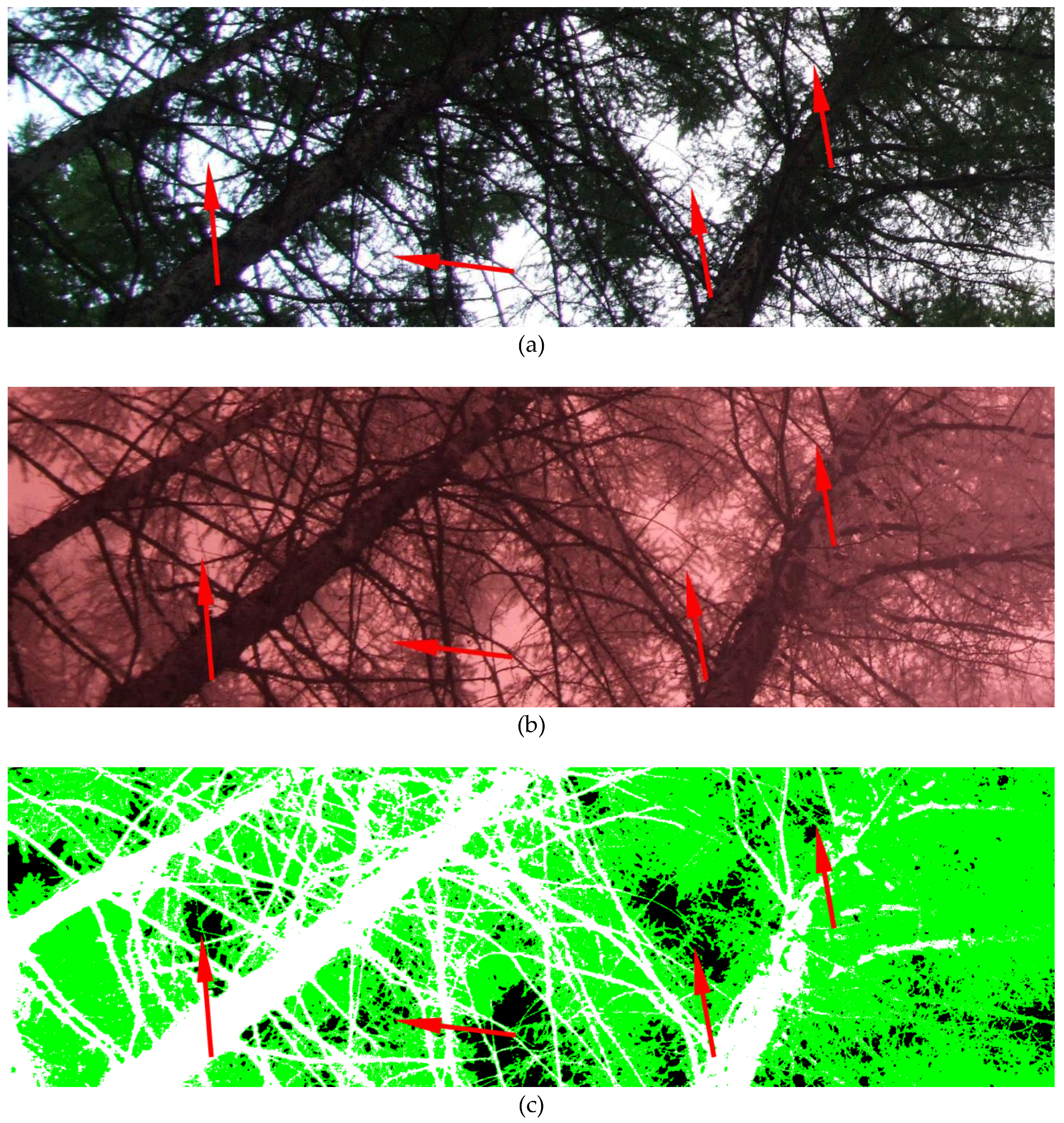
3.2.4. MCI
3.2.5. Mean Element Width, Litter Collection LAI, Corrected Needle-to-Shoot Area Ratio and Woody-to-Total Area Ratio
4. Results
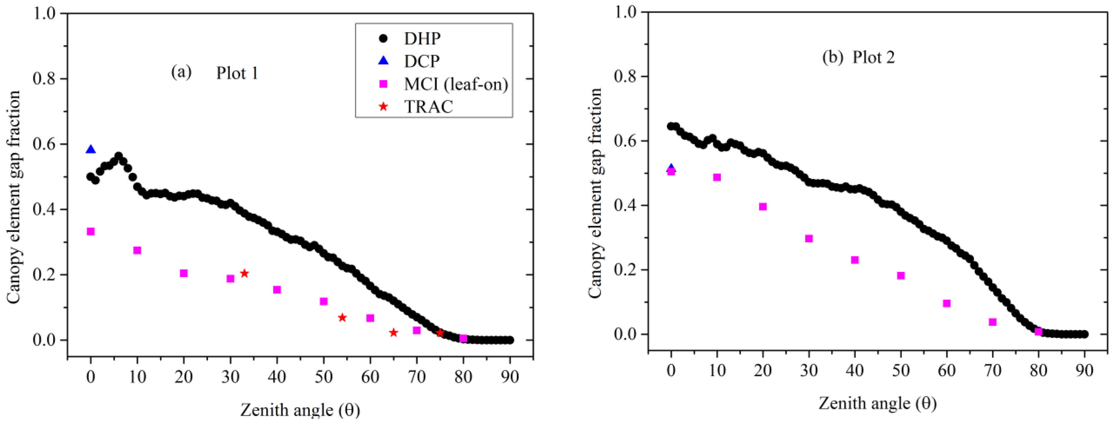
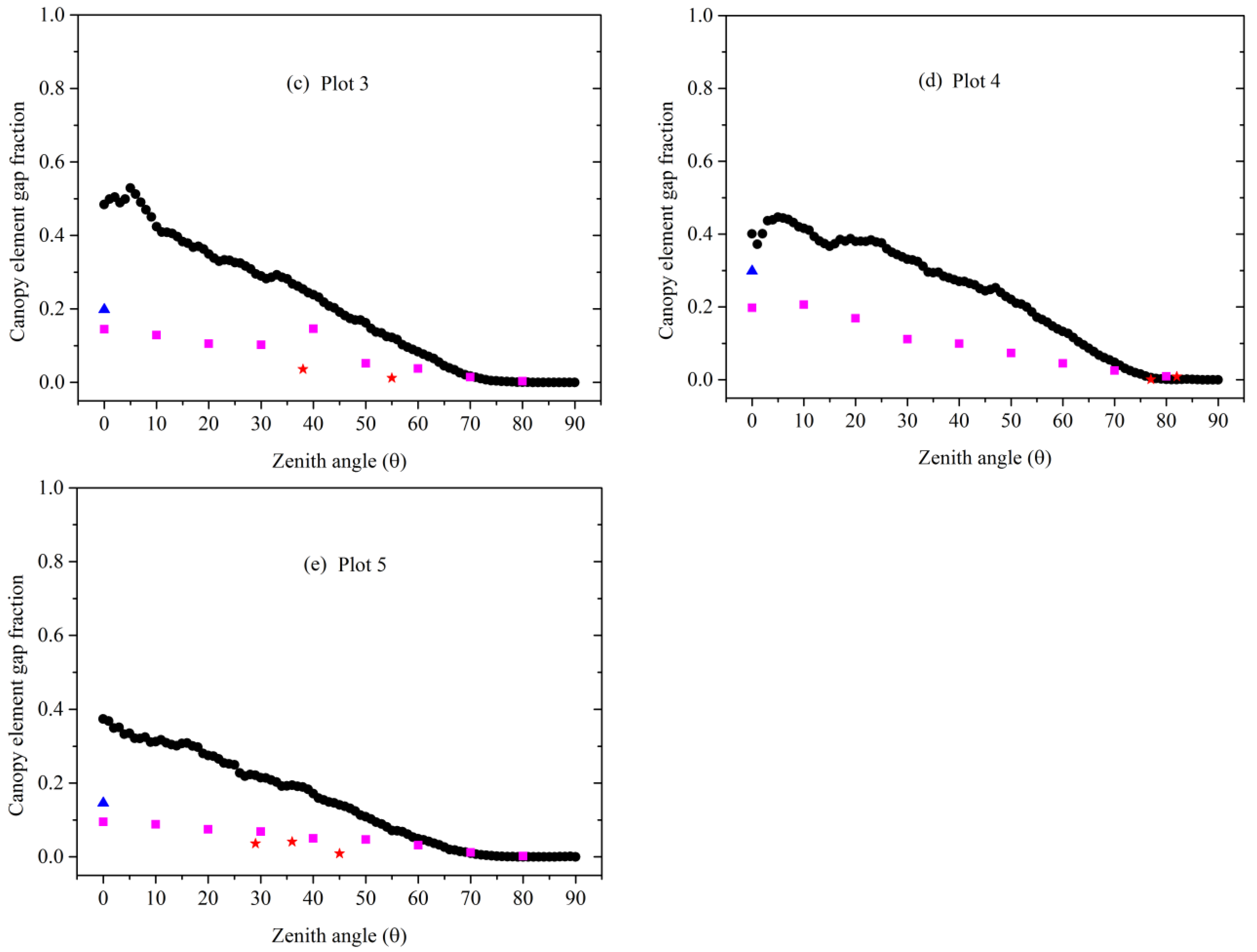
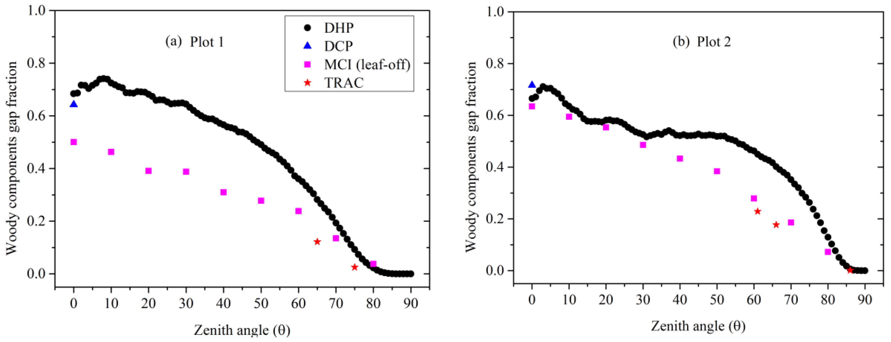
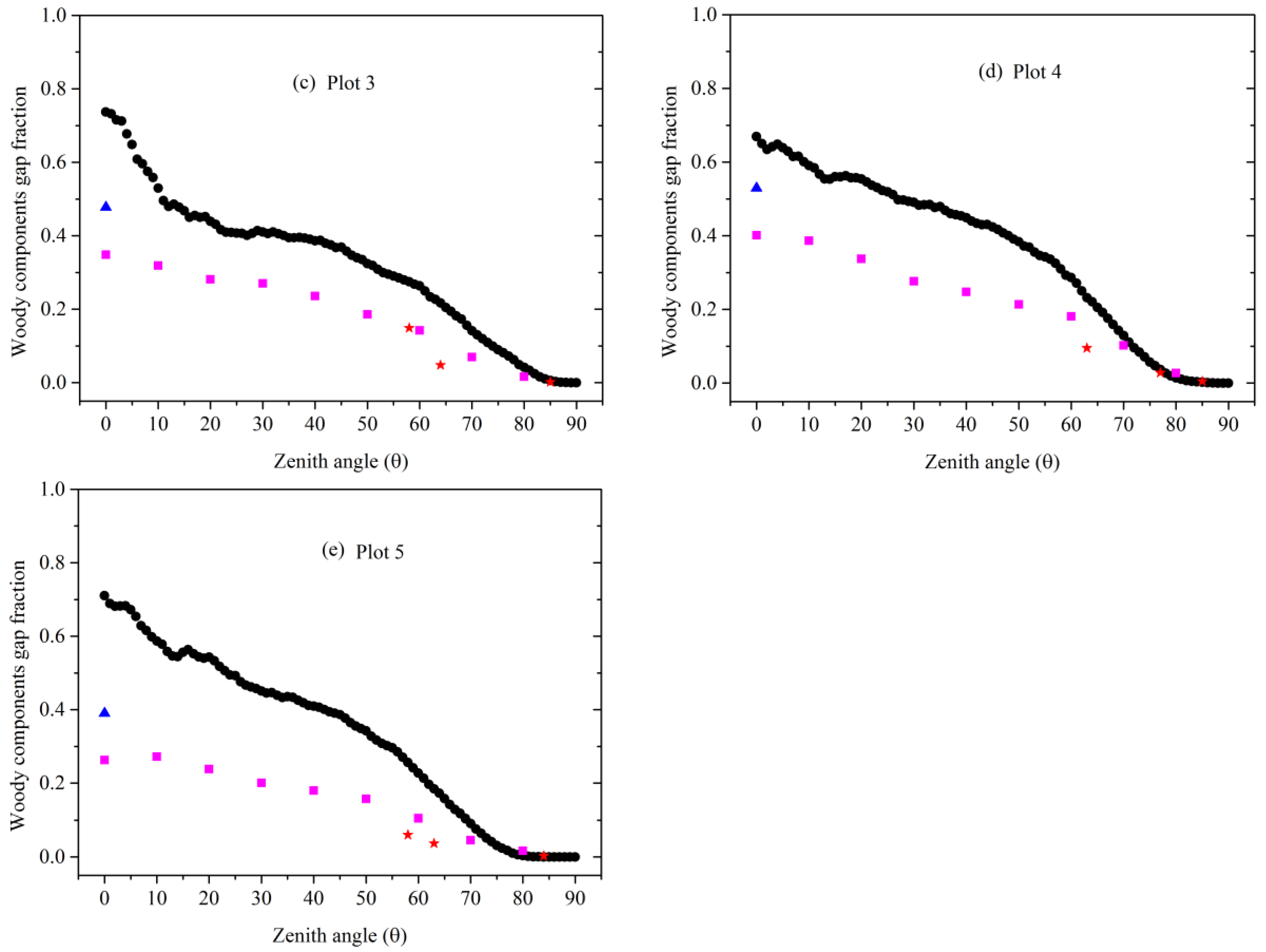
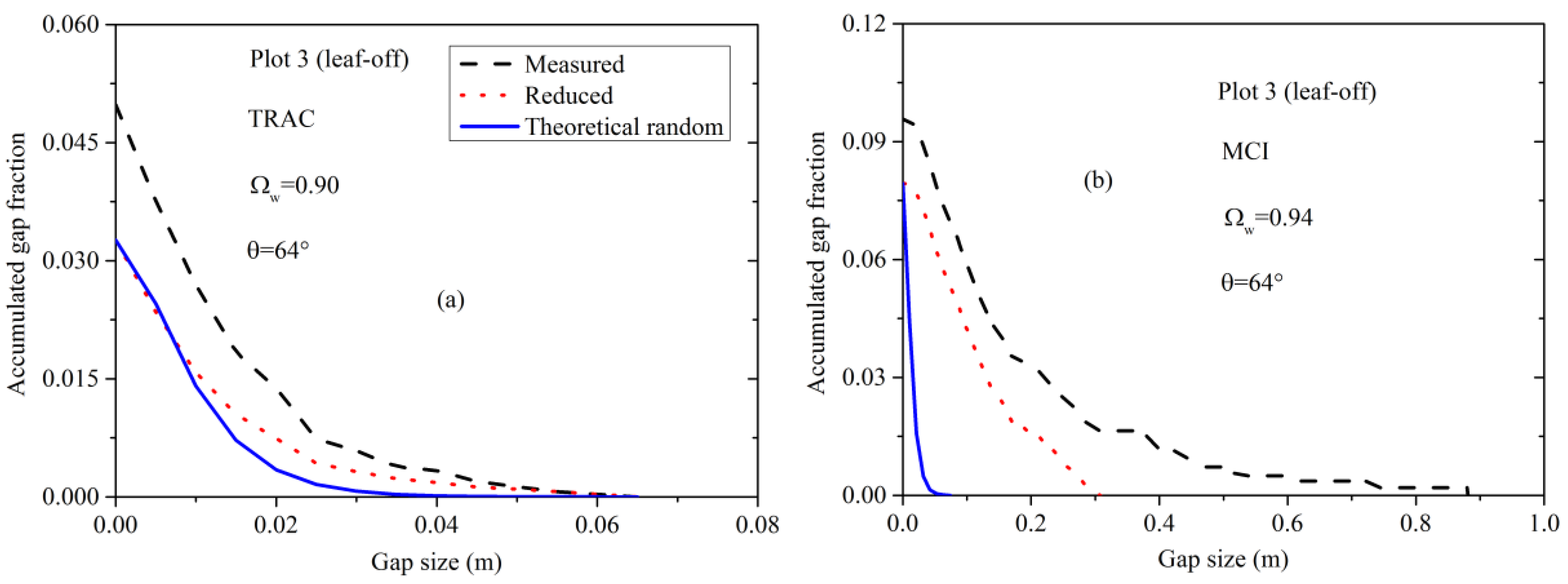
4.1. Gap Fraction
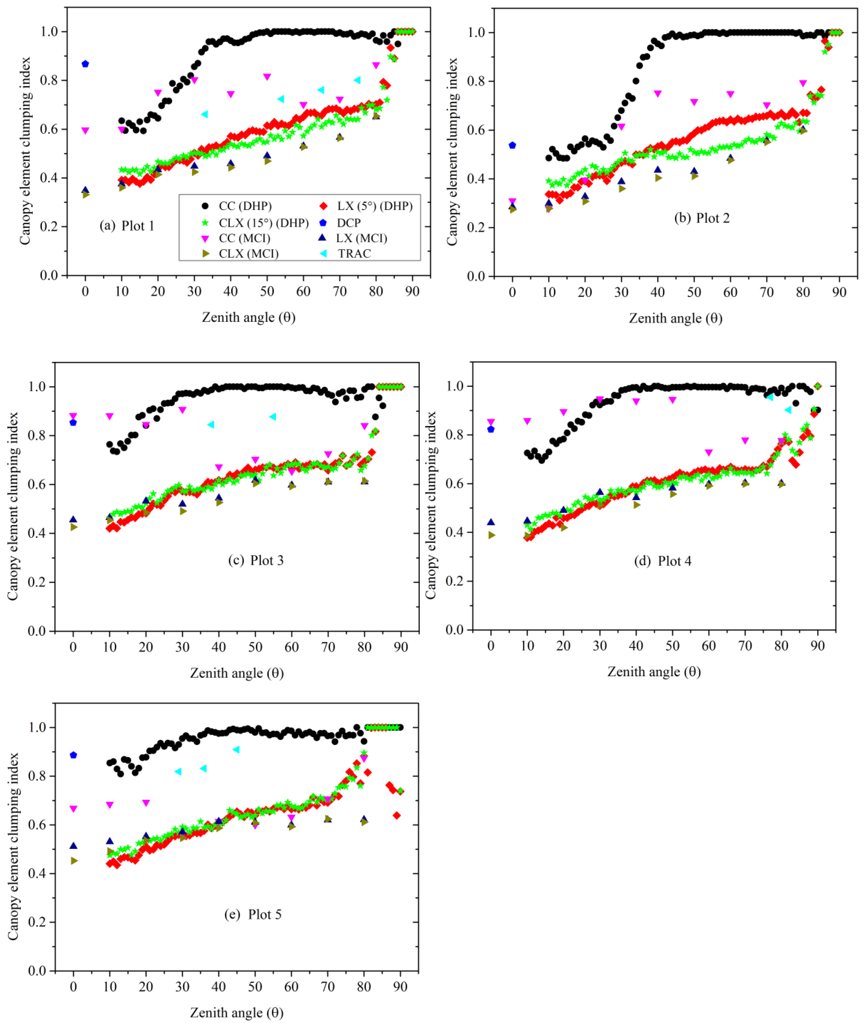
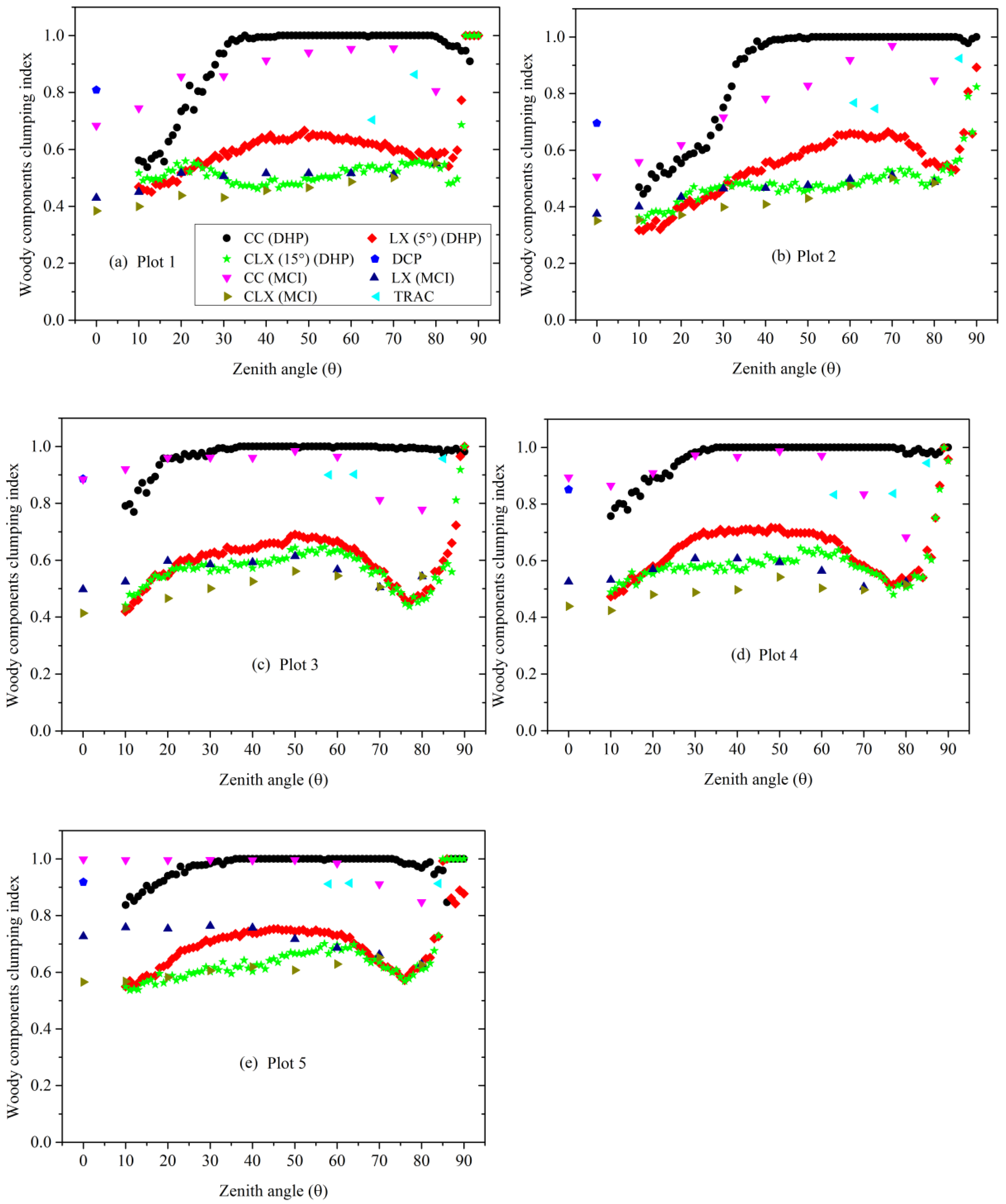
4.2. Canopy Element and Woody Components Clumping Indices
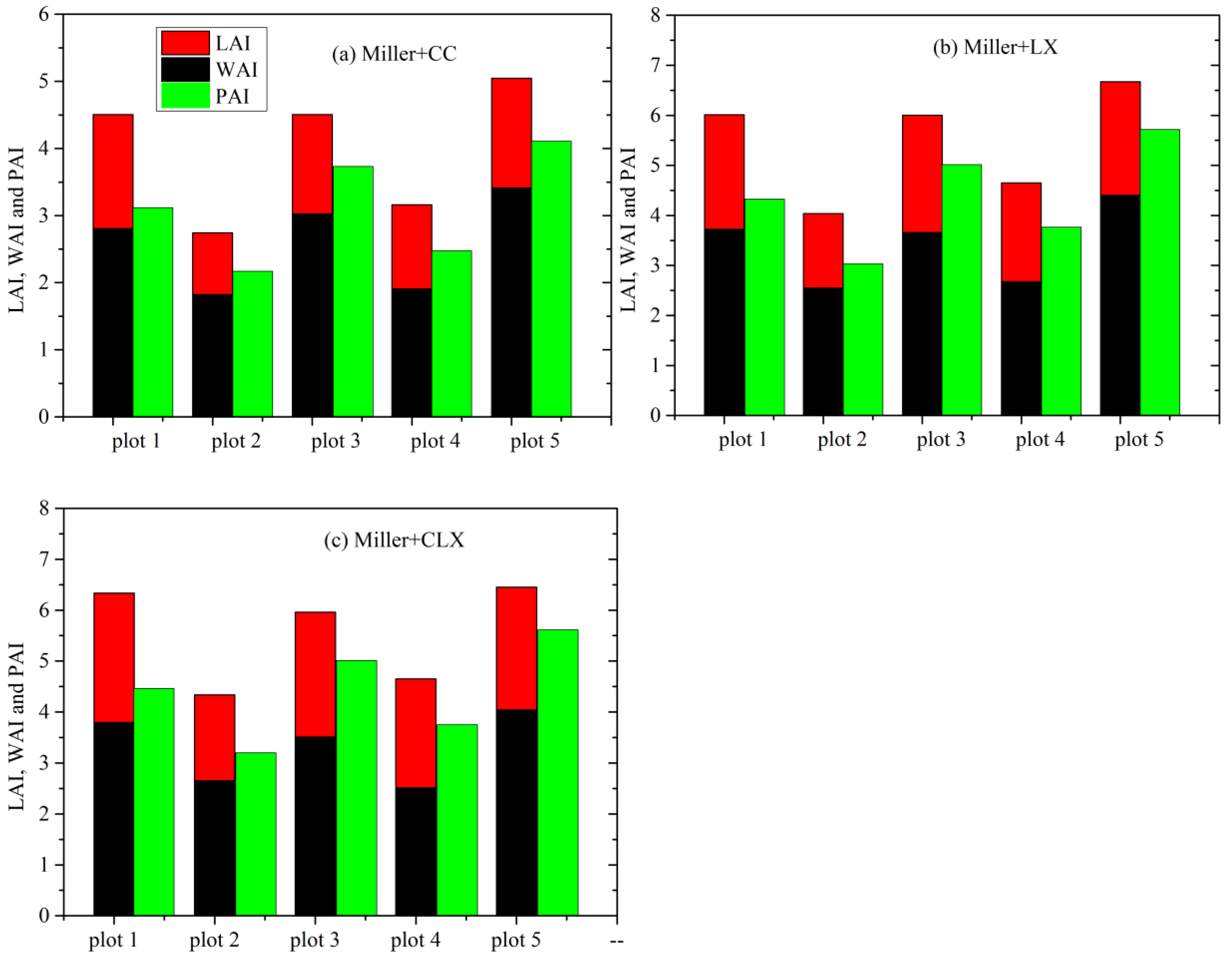
4.3. LAI
4.3.1. Canopy Element and Woody Components Clumping Index Algorithms
4.3.2. Inversion Model
4.3.3. Woody Component Correction Method
4.3.4. LAI Estimation Methods
5. Discussion
5.1. Which Canopy Element or Woody Component Clumping Index Algorithm(s) or Inversion Model(s) Is (Are) More Reliable to Be Adopted in the ESU LAI Estimation of L. principis-rupprechtii Forests from DHP and MCI?
5.2. Which Woody Components Correction Method(s) Is (Are) Better in ESU LAI Estimation for the Four Optical Methods?
5.3. Which Optical Method(s) Is (Are) More Reliable to Obtain the LAI of L. principis-rupprechtii Forest Plots?
5.4. Do the Four Optical Methods Qualify to Obtain the ESU LAI of Forests with the Accuracy Match the Requirements of GCOS?
6. Conclusions
- (1)
- using MCI and TRAC as the ESU LAI estimation methods;
- (2)
- using CC to derive the or ;
- (3)
- using the destructive or MCI woody-to-total area ratio as the woody components correction method;
- (4)
- using the Beer inversion model to derive the ESU LAI.
Author Contributions
Funding
Conflicts of Interest
Abbreviations
| half the total needle area in a shoot | |
| shoot projection area measured by projecting shoot at zenith angle 0° and azimuth angle 0° | |
| shoot projection area measured by projecting shoot at zenith angle 45° and azimuth angle 0° | |
| shoot projection area measured by projecting shoot at zenith angle 90° and azimuth angle 0° | |
| Beer | Beer inversion model (Equations (8) and (12)) |
| CC | gap size distribution algorithm |
| CLX | combination of gap size and logarithmic averaging algorithm |
| DBH | diameter at breast height |
| DCP | digital cover photography |
| DHP | digital hemispherical photography |
| ESU | elementary sampling unit |
| measured total canopy element gap fraction at | |
| total canopy element gap fraction after removing large gaps resulting from non-random distribution of canopy element at | |
| crown cover | |
| foliage cover | |
| GCOS | global climate observing system |
| canopy element projection coefficient | |
| canopy element projection coefficient at | |
| canopy element projection coefficient of ith annulus | |
| LAI | leaf area index |
| leaf area index estimated using the Beer inversion model | |
| leaf area index estimated using modified Miller theorem of LAI-2200 instrument | |
| leaf area index estimated using Miller theorem | |
| leaf area index estimated from digital cover photography method | |
| LAI-2200 | LAI-2200 inversion model (Equations (10) and (14)) |
| mean logarithmic canopy element gap fraction for all segments at | |
| LX | logarithmic averaging algorithm |
| MAE | mean absolute error |
| MCI | multispectral canopy imager |
| MCI_0-85 | modified Miller integration similar to calculation method of LAI-2200 instrument for MCI |
| Miller | Miller theorem (Equations (9) and (13)) |
| canopy element gap fraction at | |
| mean canopy element gap fraction of all segments at | |
| canopy element gap fraction of ith annulus | |
| canopy element gap fraction of segment at | |
| woody components gap fraction at | |
| woody components gap fraction of ith annulus | |
| PAI | plant area index |
| plant area index estimated using Beer inversion model | |
| plant area index estimated using modified Miller theorem of LAI-2200 instrument | |
| plant area index estimated using the MCI_0-85 inversion model | |
| plant area index estimated using Miller theorem | |
| RMSE | root mean square error |
| TRAC | tracing radiation of canopy and architecture method |
| WAI | woody area index |
| weight of ith annulus | |
| zenith angle | |
| centre zenith angle of ith annulus | |
| woody-to-total area ratio | |
| of ith annulus of MCI, which were derived using CC | |
| mean of first and second annuli of MCI, which were derived using CC | |
| needle-to-shoot area ratio | |
| corrected needle-to-shoot area ratio | |
| number of segments | |
| canopy element clumping index | |
| of ith annulus | |
| canopy element clumping index at | |
| canopy element clumping index estimated using gap size distribution algorithm at | |
| of segment at | |
| canopy element clumping index estimated from digital cover photography | |
| canopy element clumping index estimated using logarithmic averaging algorithm at | |
| canopy element clumping index estimated using a combination of gap size and logarithmic averaging algorithm at | |
| woody components clumping index | |
| woody components clumping index at | |
| crown porosity |
References
- Fang, H.; Baret, F.; Plummer, S.; Schaepman-Strub, G. An overview of global leaf area index (lai): Methods, products, validation, and applications. Rev. Geophys. 2019, 57, 739–799. [Google Scholar] [CrossRef]
- Fernandes, R.; Plummer, S.; Nightingale, J.; Baret, F.; Camacho, F.; Fang, H.; Garrigues, S.; Gobron, N.; Lang, M.; Lacaze, R.; et al. Global Leaf Area Index Product Validation Good Practices (Version 2.0); Land Product Validation Subgroup (WGCV/CEOS): Roma, Italy, 2014. [Google Scholar] [CrossRef]
- Baret, F.; Hagolle, O.; Geiger, B.; Bicheron, P.; Miras, B.; Huc, M.; Berthelot, B.; Niño, F.; Weiss, M.; Samain, O.; et al. Lai, fapar and fcover cyclopes global products derived from vegetation: Part 1: Principles of the algorithm. Remote Sens. Environ. 2007, 110, 275–286. [Google Scholar] [CrossRef]
- Masson, V.; Champeaux, J.-L.; Chauvin, F.; Meriguet, C.; Lacaze, R. A global database of land surface parameters at 1-km resolution in meteorological and climate models. J. Clim. 2003, 16, 1261–1282. [Google Scholar] [CrossRef]
- Feng, D.; Chen, J.M.; Plummer, S.; Mingzhen, C.; Pisek, J. Algorithm for global leaf area index retrieval using satellite imagery. IEEE Trans. Geosci. Remote Sens. 2006, 44, 2219–2229. [Google Scholar] [CrossRef]
- Xiao, Z.; Liang, S.; Wang, J.; Chen, P.; Yin, X.; Zhang, L.; Song, J. Use of general regression neural networks for generating the glass leaf area index product from time-series modis surface reflectance. IEEE Trans. Geosci. Remote Sens. 2014, 52, 209–223. [Google Scholar] [CrossRef]
- Knyazikhin, Y.; Martonchik, J.V.; Myneni, R.B.; Diner, D.J.; Running, S.W. Synergistic algorithm for estimating vegetation canopy leaf area index and fraction of absorbed photosynthetically active radiation from modis and misr data. J. Geophys. Res. Atmos. 1998, 103, 32257–32275. [Google Scholar] [CrossRef]
- Wenze, Y.; Dong, H.; Bin, T.; Stroeve, J.C.; Shabanov, N.V.; Knyazikhin, Y.; Nemani, R.R.; Myneni, R.B. Analysis of leaf area index and fraction of par absorbed by vegetation products from the terra modis sensor: 2000–2005. IEEE Trans. Geosci. Remote Sens. 2006, 44, 1829–1842. [Google Scholar] [CrossRef]
- Baret, F.; Weiss, M.; Lacaze, R.; Camacho, F.; Makhmara, H.; Pacholcyzk, P.; Smets, B. Geov1: Lai and fapar essential climate variables and fcover global time series capitalizing over existing products. Part1: Principles of development and production. Remote Sens. Environ. 2013, 137, 299–309. [Google Scholar] [CrossRef]
- Fang, H.; Jiang, C.; Li, W.; Wei, S.; Baret, F.; Chen, J.M.; Garcia-Haro, J.; Liang, S.; Liu, R.; Myneni, R.B.; et al. Characterization and intercomparison of global moderate resolution leaf area index (lai) products: Analysis of climatologies and theoretical uncertainties. J. Geophys. Res. Biogeosci. 2013, 118, 529–548. [Google Scholar] [CrossRef]
- Garrigues, S.; Lacaze, R.; Baret, F.; Morisette, J.T.; Weiss, M.; Nickeson, J.E.; Fernandes, R.; Plummer, S.; Shabanov, N.V.; Myneni, R.B.; et al. Validation and intercomparison of global leaf area index products derived from remote sensing data. J. Geophys. Res. Biogeosci. 2008, 113. [Google Scholar] [CrossRef]
- Jingming, C. Remote sensing of leaf area index of vegetation covers. In Remote Sensing of Natural Resources; Weng, Q., Ed.; CRC Press: Boca Raton, FL, USA, 2014; p. 24. [Google Scholar]
- Yang, X.; Zhiqiang, X.; Shunlin, L.; Jindi, W.; Jinlin, S. Validation of global land surface satellite (glass) leaf area index product. J. Remote Sens. 2014, 18, 573–596. [Google Scholar]
- Zou, J.; Yan, G.; Zhu, L.; Zhang, W. Woody-to-total area ratio determination with a multispectral canopy imager. Tree Physiol. 2009, 29, 1069–1080. [Google Scholar] [CrossRef] [PubMed]
- Woodgate, W. In-situ leaf area index estimate uncertainty in forests: Supporting earth observation product calibration and validation. Ph.D. Thesis, RMIT University, Melbourne, Australia, 2015. [Google Scholar]
- Jonckheere, I.; Fleck, S.; Nackaerts, K.; Muys, B.; Coppin, P.; Weiss, M.; Baret, F. Review of methods for in situ leaf area index determination: Part i. Theories, sensors and hemispherical photography. Agric. For. Meteorol. 2004, 121, 19–35. [Google Scholar] [CrossRef]
- Bréda, N.J.J. Ground-based measurements of leaf area index: A review of methods, instruments and current controversies. J. Exp. Bot. 2003, 54, 2403–2417. [Google Scholar] [CrossRef]
- Weiss, M.; Baret, F.; Smith, G.J.; Jonckheere, I.; Coppin, P. Review of methods for in situ leaf area index (lai) determination: Part ii. Estimation of lai, errors and sampling. Agric. For. Meteorol. 2004, 121, 37–53. [Google Scholar] [CrossRef]
- Zou, J.; Zhuang, Y.; Chianucci, F.; Mai, C.; Lin, W.; Leng, P.; Luo, S.; Yan, B. Comparison of seven inversion models for estimating plant and woody area indices of leaf-on and leaf-off forest canopy using explicit 3d forest scenes. Remote Sens. 2018, 10, 1297. [Google Scholar] [CrossRef]
- Leblanc, S.G.; Fournier, R.A. Hemispherical photography simulations with an architectural model to assess retrieval of leaf area index. Agric. For. Meteorol. 2014, 194, 64–76. [Google Scholar] [CrossRef]
- Macfarlane, C. Classification method of mixed pixels does not affect canopy metrics from digital images of forest overstorey. Agric. For. Meteorol. 2011, 151, 833–840. [Google Scholar] [CrossRef]
- Cao, B.; Du, Y.; Li, J.; Li, H.; Li, L.; Zhang, Y.; Zou, J.; Liu, Q. Comparison of five slope correction methods for leaf area index estimation from hemispherical photography. IEEE Geosci. Remote Sens. Lett. 2015, 12, 1958–1962. [Google Scholar] [CrossRef]
- Zou, J.; Leng, P.; Hou, W.; Zhong, P.; Chen, L.; Mai, C.; Qian, Y.; Zuo, Y. Evaluating two optical methods of woody-to-total area ratio with destructive measurements at five larix gmelinii rupr. Forest plots in China. Forests 2018, 9, 746. [Google Scholar] [CrossRef]
- Liu, Z.; Jin, G.; Chen, J.; Qi, Y. Evaluating optical measurements of leaf area index against litter collection in a mixed broadleaved-korean pine forest in China. Trees 2015, 29, 59–73. [Google Scholar] [CrossRef]
- Ma, L.; Zheng, G.; Eitel, J.U.H.; Magney, T.S.; Moskal, L.M. Determining woody-to-total area ratio using terrestrial laser scanning (tls). Agric. For. Meteorol. 2016, 228–229, 217–228. [Google Scholar] [CrossRef]
- Zhu, X.; Skidmore, A.K.; Wang, T.; Liu, J.; Darvishzadeh, R.; Shi, Y.; Premier, J.; Heurich, M. Improving leaf area index (lai) estimation by correcting for clumping and woody effects using terrestrial laser scanning. Agric. For. Meteorol. 2018, 263, 276–286. [Google Scholar] [CrossRef]
- Camacho, F.; Cernicharo, J.; Lacaze, R.; Baret, F.; Weiss, M. Geov1: Lai, fapar essential climate variables and fcover global time series capitalizing over existing products. Part 2: Validation and intercomparison with reference products. Remote Sens. Environ. 2013, 137, 310–329. [Google Scholar] [CrossRef]
- Baret, F.; Weiss, M.; Allard, D.; Garrigue, S.; Leroy, M.; Jeanjean, H.; Fernandes, R.; Myneni, R. VALERI: A Network of Sites and a Methodology for the Validation of Medium Spatial Resolution Satellite Products. 2005. Available online: w3.avignon.inra.fr/valeri/documents/VALERI-RSESubmitted.pdf (accessed on 18 October 2019).
- Campbell, J.L.; Burrows, S.; Gower, S.T.; Cohen, W.B. Bigfoot field manual (version 2.1). 1999. Available online: https://daac.ornl.gov/cgi-bin/dataset_lister.pl?p=1 (accessed on 18 October 2019).
- Swap, R.J.; Annegarn, H.J.; Suttles, J.T.; Haywood, J.; Helmlinger, M.C.; Hely, C.; Hobbs, P.V.; Holben, B.N.; Ji, J.; King, M.D.; et al. The southern african regional science initiative (safari 2000): Overview of the dry season field campaign. S. Afr. J. Sci. 2002, 98, 125–130. [Google Scholar]
- Gonsamo, A.; Pellikka, P. The computation of foliage clumping index using hemispherical photography. Agric. For. Meteorol. 2009, 149, 1781–1787. [Google Scholar] [CrossRef]
- Leblanc, S.G.; Chen, J.M.; Fernandes, R.; Deering, D.W.; Conley, A. Methodology comparison for canopy structure parameters extraction from digital hemispherical photography in boreal forests. Agric. For. Meteorol. 2005, 129, 187–207. [Google Scholar] [CrossRef]
- Pisek, J.; Lang, M.; Nilson, T.; Korhonen, L.; Karu, H. Comparison of methods for measuring gap size distribution and canopy nonrandomness at järvselja rami (radiation transfer model intercomparison) test sites. Agric. For. Meteorol. 2011, 151, 365–377. [Google Scholar] [CrossRef]
- Chianucci, F.; Cutini, A. Estimation of canopy properties in deciduous forests with digital hemispherical and cover photography. Agric. For. Meteorol. 2013, 168, 130–139. [Google Scholar] [CrossRef]
- Ryu, Y.; Sonnentag, O.; Nilson, T.; Vargas, R.; Kobayashi, H.; Wenk, R.; Baldocchi, D.D. How to quantify tree leaf area index in an open savanna ecosystem: A multi-instrument and multi-model approach. Agric. For. Meteorol. 2010, 150, 63–76. [Google Scholar] [CrossRef]
- Chen, J.M.; Rich, P.M.; Gower, S.T.; Norman, J.M.; Plummer, S. Leaf area index of boreal forests: Theory, techniques, and measurements. J. Geophys. Res. Atmos. 1997, 102, 29429–29443. [Google Scholar] [CrossRef]
- Lang, A.R.G.; Yueqin, X. Estimation of leaf area index from transmission of direct sunlight in discontinuous canopies. Agric. For. Meteorol. 1986, 37, 229–243. [Google Scholar] [CrossRef]
- Walter, J.-M.N.; Fournier, R.A.; Soudani, K.; Meyer, E. Integrating clumping effects in forest canopy structure: An assessment through hemispherical photographs. Can. J. Remote Sens. 2003, 29, 388–410. [Google Scholar] [CrossRef]
- Chen, J.M.; Cihlar, J. Plant canopy gap-size analysis theory for improving optical measurements of leaf-area index. Appl. Opt. 1995, 34, 6211–6222. [Google Scholar] [CrossRef]
- Chen, J.M.; Cihlar, J. Quantifying the effect of canopy architecture on optical measurements of leaf area index using two gap size analysis methods. IEEE Trans. Geosci. Remote Sens. 1995, 33, 777–787. [Google Scholar] [CrossRef]
- Macfarlane, C.; Hoffman, M.; Eamus, D.; Kerp, N.; Higginson, S.; McMurtrie, R.; Adams, M. Estimation of leaf area index in eucalypt forest using digital photography. Agric. For. Meteorol. 2007, 143, 176–188. [Google Scholar] [CrossRef]
- Chen, J.M. Optically-based methods for measuring seasonal variation of leaf area index in boreal conifer stands. Agric. For. Meteorol. 1996, 80, 135–163. [Google Scholar] [CrossRef]
- Leblanc, S.G. Correction to the plant canopy gap-size analysis theory used by the tracing radiation and architecture of canopies instrument. Appl. Opt. 2002, 41, 7667–7670. [Google Scholar] [CrossRef]
- Nilson, T. A theoretical analysis of the frequency of gaps in plant stands. Agric. For. Meteorol. 1971, 8, 25–38. [Google Scholar] [CrossRef]
- Miller, J. A formula for average foliage density. Aust. J. Bot. 1967, 15, 141–144. [Google Scholar] [CrossRef]
- LI-COR. Lai-2200 Plant Canopy Analyzer Instruction Manual; Li-cor Cor.: Lincoln, NE, USA, 2009. [Google Scholar]
- Zou, J.; Hou, W.; Zhong, P.; Zuo, Y.; Luo, S.; Leng, P. Evaluating the impact of sampling schemes on leaf area index measurements from digital hemispherical photography in Larix principis-rupprechtii Forest plots. For. Ecol. Manag. 2019. submitted. [Google Scholar]
- Sun, Z.; Liu, L.; Peng, S.; Peñuelas, J.; Zeng, H.; Piao, S. Age-related modulation of the nitrogen resorption efficiency response to growth requirements and soil nitrogen availability in a temperate pine plantation. Ecosystems 2016, 19, 698–709. [Google Scholar] [CrossRef]
- Yan, T.; Lü, X.-T.; Zhu, J.-J.; Yang, K.; Yu, L.-Z.; Gao, T. Changes in nitrogen and phosphorus cycling suggest a transition to phosphorus limitation with the stand development of larch plantations. Plant Soil 2018, 422, 385–396. [Google Scholar] [CrossRef]
- Deng, M.; Liu, L.; Sun, Z.; Piao, S.; Ma, Y.; Chen, Y.; Wang, J.; Qiao, C.; Wang, X.; Li, P. Increased phosphate uptake but not resorption alleviates phosphorus deficiency induced by nitrogen deposition in temperate larix principis-rupprechtii plantations. New Phytol. 2016, 212, 1019–1029. [Google Scholar] [CrossRef] [PubMed]
- Gonsamo, A.; Pellikka, P. Methodology comparison for slope correction in canopy leaf area index estimation using hemispherical photography. For. Ecol. Manag. 2008, 256, 749–759. [Google Scholar] [CrossRef]
- Zou, J.; Yan, G.; Chen, L. Estimation of canopy and woody components clumping indices at three mature Picea crassifolia forest stands. IEEE J. Sel. Top. Appl. Earth Obs. Remote Sens. 2015, 8, 1413–1422. [Google Scholar] [CrossRef]
- Leblanc, S.G.; Chen, J.M.; Kwong, M. Tracing Radiation and Architecture of Canopies Trac Manual (Version 2.1.3); Natural Resources Canada: Ottawa, ON, Canada, 2002; p. 25.
- Gonsamo, A.; Walter, J.-M.N.; Pellikka, P. Sampling gap fraction and size for estimating leaf area and clumping indices from hemispherical photographs. Can. J. Forest Res. 2010, 40, 1588–1603. [Google Scholar] [CrossRef]
- Gower, S.T.; Kucharik, C.J.; Norman, J.M. Direct and indirect estimation of leaf area index, fapar, and net primary production of terrestrial ecosystems. Remote Sens. Environ. 1999, 70, 29–51. [Google Scholar] [CrossRef]
- Calders, K.; Origo, N.; Disney, M.; Nightingale, J.; Woodgate, W.; Armston, J.; Lewis, P. Variability and bias in active and passive ground-based measurements of effective plant, wood and leaf area index. Agric. For. Meteorol. 2018, 252, 231–240. [Google Scholar] [CrossRef]
- Cutini, A.; Matteucci, G.; Mugnozza, G.S. Estimation of leaf area index with the li-cor LAI-2000 in deciduous forests. For. Ecol. Manag. 1998, 105, 55–65. [Google Scholar] [CrossRef]
- Toda, M.; Richardson, A.D. Estimation of plant area index and phenological transition dates from digital repeat photography and radiometric approaches in a hardwood forest in the northeastern united states. Agric. For. Meteorol. 2018, 249, 457–466. [Google Scholar] [CrossRef]
- Pisek, J.; Sonnentag, O.; Richardson, A.D.; Mõttus, M. Is the spherical leaf inclination angle distribution a valid assumption for temperate and boreal broadleaf tree species? Agric. For. Meteorol. 2013, 169, 186–194. [Google Scholar] [CrossRef]
- Raabe, K.; Pisek, J.; Sonnentag, O.; Annuk, K. Variations of leaf inclination angle distribution with height over the growing season and light exposure for eight broadleaf tree species. Agric. For. Meteorol. 2015, 214–215, 2–11. [Google Scholar] [CrossRef]
- Kucharik, C.J.; Norman, J.M.; Murdock, L.M.; Gower, S.T. Characterizing canopy nonrandomness with a multiband vegetation imager (mvi). J. Geophys. Res. Atmos. 1997, 102, 29455–29473. [Google Scholar] [CrossRef]
- Knipling, E.B. Physical and physiological basis for the reflectance of visible and near-infrared radiation from vegetation. Remote Sens. Environ. 1970, 1, 155–159. [Google Scholar] [CrossRef]
- Chapman, L. Potential applications of near infra-red hemispherical imagery in forest environments. Agric. For. Meteorol. 2007, 143, 151–156. [Google Scholar] [CrossRef]
- Raabe, K.; Pisek, J.; Lang, M.; Korhonen, L. Estimating the beyond-shoot foliage clumping at two contrasting points in the growing season using a variety of field-based methods. Trees 2017, 31, 1367–1373. [Google Scholar] [CrossRef]
- Law, B.E.; Van Tuyl, S.; Cescatti, A.; Baldocchi, D.D. Estimation of leaf area index in open-canopy ponderosa pine forests at different successional stages and management regimes in oregon. Agric. For. Meteorol. 2001, 108, 1–14. [Google Scholar] [CrossRef]
- van Gardingen, P.R.; Jackson, G.E.; Hernandez-Daumas, S.; Russell, G.; Sharp, L. Leaf area index estimates obtained for clumped canopies using hemispherical photography. Agric. For. Meteorol. 1999, 94, 243–257. [Google Scholar] [CrossRef]


| Equations | References | |
|---|---|---|
| (1) | [43] | |
| (2) | [37] | |
| (3) | [32] | |
| (4) | [41] | |
| (5) | [42] | |
| (6) | [14] | |
| Equations | References | |
|---|---|---|
| PAI | (7) | [44] |
| (8) | [19,44] | |
| (9) | [45] | |
| (10) | [19,46] | |
| (11) | [23] | |
| (12) | [19,44] | |
| (13) | ||
| (14) | [19,46] | |
| (15) | [41] | |
| Plot 1 | Plot 2 | Plot 3 | Plot 4 | Plot 5 | |
|---|---|---|---|---|---|
| Longitude and latitude | 42°24′43″ N, 117°19′4″ E | 42°24′2″ N, 117°18′40″ E | 42°18′2″ N, 117°18′9″ E | 42°25′22″ N, 117°19′32″ E | 42°17′42″ N, 117°16′53″ E |
| Mean tree height (m) | 19.43 | 20.4 | 12.58 | 13.31 | 8.73 |
| Average DBH (cm) | 26.58 | 27.22 | 12.71 | 14.14 | 9.23 |
| Mean element width (mm) | 21.66 | 23.34 | 17.91 | 21.09 | 17.60 |
| Stand density (stems/ha) | 464 | 384 | 2320 | 1760 | 3904 |
| Tree age (approximate years) | 54 | 55 | 21 | 22 | 13 |
| Corrected needle-to-shoot area ratio () | 1.30 | 1.17 | 1.14 | 1.17 | 1.28 |
| Woody-to-total area ratio () | 0.16 | 0.16 | 0.20 | 0.24 | 0.23 |
| Litter collection LAI | 4.65 | 3.58 | 4.96 | 3.04 | 6.69 |
| Slope | ~0° | ||||
| Tree species | Larix principis-rupprechtii | ||||
| WAI Obtained from Leaf-off DHP Images | ||||||||||||||||
|---|---|---|---|---|---|---|---|---|---|---|---|---|---|---|---|---|
| Inversion Model | Plot 1 | Plot 2 | Plot 3 | Plot 4 | Plot 5 | Plot 1 | Plot 2 | Plot 3 | Plot 4 | Plot 5 | Plot 1 | Plot 2 | Plot 3 | Plot 4 | Plot 5 | |
| Beer | CC | 1.93 | 1.25 | 2.26 | 1.80 | 3.00 | 2.07 | 1.25 | 2.28 | 1.82 | 3.24 | 1.31 | 0.69 | 1.42 | 1.1 | 2.45 |
| LX | 3.04 | 1.98 | 3.34 | 2.77 | 4.40 | 3.11 | 1.98 | 3.05 | 2.59 | 4.40 | 2.07 | 1.11 | 2.09 | 1.82 | 3.75 | |
| CLX | 3.30 | 2.38 | 3.37 | 2.86 | 4.38 | 3.34 | 2.35 | 2.95 | 2.52 | 4.10 | 2.01 | 1.15 | 1.99 | 1.74 | 3.55 | |
| Miller | CC | 2.62 | 1.82 | 2.99 | 1.88 | 3.16 | 2.81 | 1.82 | 3.02 | 1.91 | 3.41 | 1.42 | 1.25 | 2.25 | 1.22 | 2.47 |
| LX | 3.64 | 2.55 | 4.01 | 2.86 | 4.40 | 3.72 | 2.55 | 3.66 | 2.67 | 4.40 | 2.04 | 1.54 | 2.67 | 1.79 | 3.45 | |
| CLX | 3.75 | 2.69 | 4.01 | 2.85 | 4.32 | 3.79 | 2.66 | 3.51 | 2.51 | 4.04 | 1.92 | 1.52 | 2.56 | 1.62 | 3.21 | |
| LAI-2200 | CC | 1.99 | 1.41 | 2.18 | 1.83 | 2.87 | 2.14 | 1.41 | 2.21 | 1.85 | 3.09 | 1.38 | 0.68 | 1.29 | 1.12 | 2.29 |
| LX | 3.19 | 2.22 | 3.37 | 2.96 | 4.41 | 3.27 | 2.22 | 3.07 | 2.77 | 4.41 | 2.25 | 1.04 | 2.28 | 1.95 | 3.68 | |
| CLX | 3.32 | 2.39 | 3.37 | 2.96 | 4.33 | 3.36 | 2.36 | 2.95 | 2.61 | 4.05 | 2.13 | 1.01 | 1.79 | 1.75 | 3.4 | |
| WAI Obtained from Leaf-off DHP Images | |||||||||||||||||||
|---|---|---|---|---|---|---|---|---|---|---|---|---|---|---|---|---|---|---|---|
| Inversion Model | RMSE (%) | MAE (%) | R2 | Intercept | Slope | p | RMSE (%) | MAE (%) | R2 | Intercept | Slope | p | RMSE (%) | MAE (%) | R2 | Intercept | Slope | p | |
| Beer | CC | 2.66 (58%) | 2.54 (55%) | 0.90 | 0.17 | 0.41 | 0.04 | 2.56 (56%) | 2.45 (53%) | 0.91 | −0.03 | 0.47 | 0.03 | 3.28 (72%) | 3.19 (70%) | 0.92 | −0.55 | 0.42 | 0.03 |
| LX | 1.62 (35%) | 1.48 (31%) | 0.89 | 0.54 | 0.56 | 0.04 | 1.67 (37%) | 1.56 (33%) | 0.92 | 0.36 | 0.58 | 0.03 | 2.50 (54%) | 2.42 (53%) | 0.89 | −0.63 | 0.61 | 0.04 | |
| CLX | 1.49 (33%) | 1.33 (27%) | 0.93 | 1.01 | 0.49 | 0.02 | 1.69 (37%) | 1.53 (32%) | 0.94 | 0.92 | 0.47 | 0.02 | 2.58 (56%) | 2.50 (55%) | 0.9 | −0.51 | 0.57 | 0.04 | |
| Miller | CC | 2.23 (49%) | 2.09 (45%) | 0.92 | 0.64 | 0.40 | 0.03 | 2.11 (46%) | 1.99 (43%) | 0.94 | 0.45 | 0.47 | 0.02 | 2.98 (65%) | 2.86 (62%) | 0.9 | −0.01 | 0.38 | 0.04 |
| LX | 1.29 (28%) | 1.09 (22%) | 0.92 | 1.17 | 0.51 | 0.03 | 1.34 (29%) | 1.18 (24%) | 0.96 | 0.98 | 0.53 | 0.01 | 2.38 (52%) | 2.29 (50%) | 0.94 | −0.06 | 0.51 | 0.02 | |
| CLX | 1.28 (28%) | 1.06 (21%) | 0.92 | 1.37 | 0.47 | 0.03 | 1.48 (32%) | 1.28 (26%) | 0.92 | 1.27 | 0.44 | 0.03 | 2.51 (55%) | 2.42 (53%) | 0.95 | −0.03 | 0.48 | 0.01 | |
| LAI-2200 | CC | 2.67 (58%) | 2.53 (54%) | 0.91 | 0.47 | 0.35 | 0.03 | 2.57 (56%) | 2.44 (53%) | 0.92 | 0.3 | 0.4 | 0.03 | 3.33 (73%) | 3.23 (71%) | 0.9 | −0.37 | 0.38 | 0.04 |
| LX | 1.53 (33%) | 1.35 (28%) | 0.89 | 0.95 | 0.50 | 0.04 | 1.59 (35%) | 1.44 (30%) | 0.91 | 0.76 | 0.52 | 0.03 | 2.43 (53%) | 2.34 (51%) | 0.88 | −0.46 | 0.59 | 0.05 | |
| CLX | 1.50 (33%) | 1.31 (26%) | 0.91 | 1.18 | 0.46 | 0.03 | 1.69 (37%) | 1.52 (31%) | 0.92 | 1.08 | 0.43 | 0.03 | 2.67 (58%) | 2.57 (56%) | 0.86 | −0.43 | 0.53 | 0.06 | |
| Leaf-on MCI Images | Leaf-on and Leaf-off MCI Images | ||||||||||
|---|---|---|---|---|---|---|---|---|---|---|---|
| Inversion Model | Plot 1 | Plot 2 | Plot 3 | Plot 4 | Plot 5 | Plot 1 | Plot 2 | Plot 3 | Plot 4 | Plot 5 | |
| Beer | CC | 4.92 | 3.53 | 5.21 | 4.41 | 6.47 | 3.80 | 2.48 | 4.02 | 3.50 | 5.11 |
| LX | 6.12 | 5.28 | 4.94 | 4.79 | 6.23 | 4.17 | 3.38 | 3.07 | 3.31 | 4.45 | |
| CLX | 6.09 | 5.30 | 4.74 | 4.58 | 6.01 | 4.03 | 3.34 | 2.98 | 2.99 | 4.20 | |
| MCI_0-85 | CC | 3.77 | 3.10 | 3.71 | 2.94 | 5.63 | 2.57 | 2.15 | 2.50 | 1.89 | 4.40 |
| LX | 5.40 | 4.28 | 4.40 | 4.04 | 5.57 | 3.48 | 2.70 | 2.65 | 2.66 | 4.17 | |
| CLX | 5.48 | 4.40 | 4.33 | 4.08 | 5.34 | 3.41 | 2.71 | 2.52 | 2.61 | 3.84 | |
| Leaf-on MCI Images | Leaf-on and Leaf-off MCI Images | ||||||||||||
|---|---|---|---|---|---|---|---|---|---|---|---|---|---|
| Inversion Model | RMSE (%) | MAE (%) | R2 | Intercept | Slope | p | RMSE (%) | MAE (%) | R2 | Intercept | Slope | p | |
| Beer | CC | 0.64 (14%) | 0.43 (12%) | 0.91 | 1.71 | 0.70 | 0.03 | 1.05 (23%) | 0.99 (21%) | 0.86 | 1.12 | 0.58 | 0.06 |
| LX | 1.29 (28%) | 1.08 (29%) | 0.71 | 3.93 | 0.34 | 0.18 | 1.34 (29%) | 1.02 (19%) | 0.68 | 2.36 | 0.29 | 0.21 | |
| CLX | 1.26 (27%) | 1.12 (29%) | 0.62 | 3.94 | 0.31 | 0.26 | 1.45 (32%) | 1.08 (20%) | 0.70 | 2.21 | 0.28 | 0.19 | |
| MCI_0-85 | CC | 0.86 (19%) | 0.75 (15%) | 0.97 | 0.47 | 0.73 | 0.01 | 1.95 (43%) | 1.88 (41%) | 0.95 | −0.34 | 0.66 | 0.01 |
| LX | 0.85 (19%) | 0.83 (19%) | 0.81 | 2.89 | 0.40 | 0.09 | 1.67 (36%) | 1.45 (29%) | 0.83 | 1.30 | 0.40 | 0.08 | |
| CLX | 0.97 (21%) | 0.93 (22%) | 0.70 | 3.28 | 0.32 | 0.19 | 1.82 (40%) | 1.57 (31%) | 0.77 | 1.58 | 0.31 | 0.13 | |
| Plot 1 | Plot 2 | Plot 3 | Plot 4 | Plot 5 | |
|---|---|---|---|---|---|
| Leaf-on DCP images | 1.44 | 2.35 | 3.89 | 2.81 | 4.92 |
| Leaf-on and leaf-off DCP images | 0.53 | 1.94 | 2.66 | 1.95 | 3.5 |
| RMSE (%) | MAE (%) | R2 | Intercept | Slope | p | |
|---|---|---|---|---|---|---|
| Leaf-on DCP images | 1.80 (39%) | 1.50 (32%) | 0.68 | 0.08 | 0.65 | 0.20 |
| Leaf-on and leaf-off DCP images | 2.70 (59%) | 2.47 (53%) | 0.56 | 0.13 | 0.43 | 0.33 |
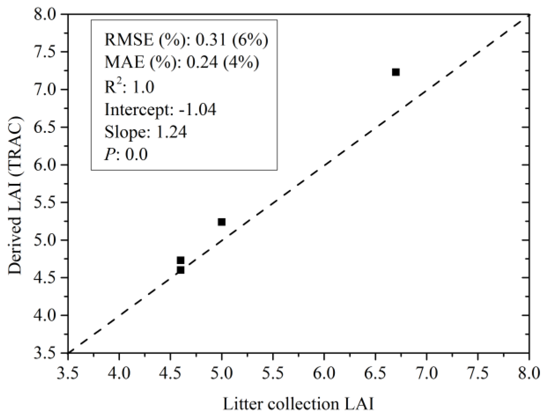
| Plot 1 | Plot 3 | Plot 5 | ||
|---|---|---|---|---|
| 54.1° | 64.85° | 55.25° | 44.9° | |
| LAI | 4.73 | 4.60 | 5.24 | 7.23 |
© 2019 by the authors. Licensee MDPI, Basel, Switzerland. This article is an open access article distributed under the terms and conditions of the Creative Commons Attribution (CC BY) license (http://creativecommons.org/licenses/by/4.0/).
Share and Cite
Zou, J.; Zuo, Y.; Zhong, P.; Hou, W.; Leng, P.; Chen, B. Performance of Four Optical Methods in Estimating Leaf Area Index at Elementary Sampling Unit of Larix principis-rupprechtii Forests. Forests 2020, 11, 30. https://doi.org/10.3390/f11010030
Zou J, Zuo Y, Zhong P, Hou W, Leng P, Chen B. Performance of Four Optical Methods in Estimating Leaf Area Index at Elementary Sampling Unit of Larix principis-rupprechtii Forests. Forests. 2020; 11(1):30. https://doi.org/10.3390/f11010030
Chicago/Turabian StyleZou, Jie, Yong Zuo, Peihong Zhong, Wei Hou, Peng Leng, and Bin Chen. 2020. "Performance of Four Optical Methods in Estimating Leaf Area Index at Elementary Sampling Unit of Larix principis-rupprechtii Forests" Forests 11, no. 1: 30. https://doi.org/10.3390/f11010030
APA StyleZou, J., Zuo, Y., Zhong, P., Hou, W., Leng, P., & Chen, B. (2020). Performance of Four Optical Methods in Estimating Leaf Area Index at Elementary Sampling Unit of Larix principis-rupprechtii Forests. Forests, 11(1), 30. https://doi.org/10.3390/f11010030