Abstract
Estimation of forestry aboveground biomass (AGB) by means of aerial Light Detection and Ranging (LiDAR) data uses high-density point sampling data obtained in dedicated flights, which are often too costly for available research budgets. In this paper we exploit already existing public low-density LiDAR data obtained for other purposes, such as cartography. The challenge is to show that such low-density data allows accurate biomass estimation. We demonstrate the approach on data available from plantations of Pinus radiata in the Arratia-Nervión region, located in Biscay province located in the North of Spain. We use public data gathered from the low-density (0.5 pulse/m2) LiDAR flight conducted by the Basque Government in 2012 for cartographic production. We propose a linear regression model based on explanatory variables obtained from the LiDAR point cloud data. We calibrate the model using field data from the Fourth National Forest Inventory (NFI4), including the selection of the optimal model variables. The results revealed that the best model depends on two variables extracted from LiDAR data: One directly related with tree height and a second parameter with the canopy density. The model explained 80% of its variability with a standard error of 0.25 ton/ha in logarithmic units. We validate the predictions against the biomass measurements provided by the government institutions, obtaining a difference of 8%. The proposed approach would allow the exploitation of the periodic available low-density LiDAR data, collected with territorial and cartographic purposes, for a more frequent and less expensive control of the forestry biomass.
1. Introduction
Assessing forest resources has gained increased attention by governments worldwide in the last few decades due to increased awareness about global climate change, and a greater appreciation of the ecosystem services provided by forests [1]. Forests play a dual role in the global carbon cycle: (i) As an important carbon sink removing carbon dioxide through photosynthesis and converting the photosynthate to forest biomass; and (ii) as a carbon source by releasing carbon dioxide through respiration, wildfires, and decomposition [2]. Thus, there is great uncertainty over whether forests will be a carbon sink or source in the future. If forests are well managed, and timber is used for long-term products such as buildings, then forest management will result in a net reduction of atmospheric carbon. On the contrary, burning wood for agriculture, residential, and commercial uses will increase carbon emission rates [2].
Pinus radiata (D. Don) is native to the Californian coastal environment. It is the most extensively planted coniferous species in the Southern Hemisphere covering a total area exceeding 4.3 million ha and still expanding. It is a major species cultivated for timber production in Australia, Chile, New Zealand, South Africa, and Spain [3]. The worldwide P. radiata forest resource provides substantial carbon storage through continued atmospheric carbon sequestration as plantations grow accumulating biomass. Estimated P. radiata carbon storage in some regions [4] serve as an indication of the magnitude of environmental services that P. radiata plantations can provide by terrestrial carbon sinks to offset carbon emissions.
The provinces of the Atlantic area in the north of Spain contain more than 90% of the P. radiata cover of the country (about 260,000 ha), almost half (47%) of it is located in the Basque Country. P. radiata is not native to the region. It was first introduced in the late 1800s. Two main repopulations were carried out since, one at the middle of the 1920s, and a second which was more intensive in the 1940s [5]. The primary reasons for its fast penetration in the region are: Its great growth in temperate humid climates; and the versatility of its wood, which is suitable for various industrial uses, and obtaining large harvest quantities. Additional benefits are (a) its adaptability to different environments without large production losses (plasticity); (b) the relative absence of pests or serious diseases that impede their development in large areas; and (c) its silvicultural flexibility, that is, the possibility of practicing different silvicultural processes without diminishing the production [5].
According to the latest Spanish National Forest Inventory (NFI4), carried out in 2011, 68% of the Basque Country land cover are forests. The Basque Country is the Spanish autonomous community with the highest density of timber stocks in Spain. The average density reported in the NFI4 is higher than 160 m3/ha. The importance of P. radiata in Spain is due to its high productivity: It is only 0.7% of the national forested area; however, the outcome of this species is approximately 7% of the total wood production made in Spain [6].
Forest ecosystem management needs a multi-faceted approach, combining forest mapping and inventory in order to provide comprehensive knowledge on the current state and future trends of forest resources, as well as on their interactions and interdependencies with other land uses [7]. Such approach needs a statistical framework integrating data from multiple sources, such as remotely-sensed and sample inventory data [8], using approximately unbiased model-assisted estimators. Allometric equations relate easily measurable forest variables (tree diameter and height) with the biomass obtained in the field by destructive sampling methods. They have been shown to be useful tools for forest management. In this paper, we use the allometric equation results reported by the HAZI foundation (HAZI is a research organization funded by the Basque Government devoted to the sustainable exploitation of natural resources https://www.hazi.eus/es/) for validation of our proposal.
Even if forest inventory and mapping meet different information needs, support for forest ecosystem management should therefore be framed according to a multi-faceted approach that combines forest mapping and inventory as a means of providing comprehensive knowledge on the state and trends of forest resources, as well as on their interactions and interdependencies with other land uses [7]. Such integration can be based on an effective statistical framework from multiple perspectives such as coupling remotely-sensed and sample inventory data for different purposes [8], using approximately unbiased model-assisted estimators.
Remotely acquired data (land, airborne, or satellite based) have been successfully used for the assessment of tree characteristics [9,10,11,12]. Light detection and ranging (LiDAR) stands out among the available remote sensing methods for several reasons. First, it allows the acquisition of data in large areas. Secondly, it provides measures of variables describing the structure of the forest canopy (average height, dominant height, or mean diameter) [13,14,15], even allowing the discrimination between tree species [16]. Forest biomass can be estimated on the basis of these variables by diverse approaches [17,18,19,20], which can be categorized depending on the footprint size and the object under study (plot size or individual tree). Early studies used small-footprint (discrete) LiDAR data to estimate biophysical properties of forest stands at plot size. They started in the 1980s using profiling lasers [21]. Later approaches measure the strength of the return of the laser pulse at each sample point, which depends on the surface reflectivity. The increase of the pulse frequency in modern LiDAR systems provides an increase of pulse density, allowing to detect treetops, gaps between the forest crowns, and individual tree analysis [22,23]. Full-waveform systems capturing the returned energy in an almost continuous fashion have been used highly accurate biomass estimation [24,25].
Specific LiDAR data capture campaigns for biomass measurement are very expensive, hindering the general application of the technology in forestry management. However, this obstacle can be overcome. Some institutions carry out periodic LiDAR data capture campaigns to build digital terrain and surface models, mostly for cartographic purposes. These datasets are published by the administration institutions, such as the Basque Government, and can be exploited for other applications [26]. The main disadvantage of these datasets are their low sampling density (0.5 pulse/m2).
The purpose of this paper is to show that these low-density datasets can be useful for forest biomass estimation; therefore, allowing for their systematic use in forest management. We develop a linear regression model to estimate aboveground biomass (AGB) after optimal selection of LiDAR data features using the HAZI’s allometric equations for P. radiata applied over the NFI4 data for validation purposes. The specific dataset used to demonstrate our approach is a low sampling density LiDAR dataset covering the whole area of Spain collected in the National Plan of Aerial Orthophotography (PNOA) carried out in 2011.
2. Materials and Methods
2.1. Study Area
The study area is the Arratia-Nervión region, located in the province of Biscay (Basque Country), in the northern part of Spain (Figure 1). This region encompasses 14 municipalities, covering a total area of 400 km2. The average altitude of the region is 465 m, with an average slope of 18.6°. High slope (30–45°) areas are frequent across the entire region.
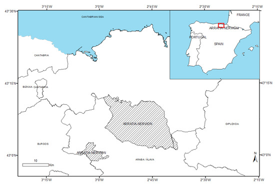
Figure 1.
Inset: Localization in the Spain country. Picture: Arratia-Nervión region (dashed) in Basque Country, Spain.
Pine forests of P. radiata are the most important land cover in the Basque Country, 125,000 ha, accounting for 32% of the forested area in the Basque Country, equivalent to 49% of the area covered by this species in Spain. These pine forests provide 23% of the volume of large trees in the Basque Country, and 44% of the volume including bark. Forests of P. radiata are cultivated at altitudes below 600 m.
According to the NFI4, in Arratia-Nervión 16,260 ha out of 28,065 ha of forest areas belong to the P. radiata D. Don. tree species, representing over 60% of the tree specimens of the area (Figure 2). Coniferous plantations have progressively replaced the native tree species. The only invading species is the Robinia pseudoacacia with a minor presence of 17 ha in the entire region. Native species, such as Quercus ilex or Fagus sylvatica, represent only 12.5% (3511 ha) of the total forested areas in the region.
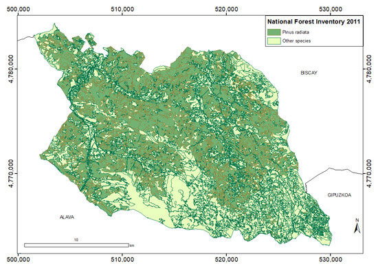
Figure 2.
P. radiata distribution (in green) in the Arratia-Nervión region (ETRS89 UTM zone 30 North reference system).
2.2. Field Data Collection
The dendrometric data used in this study were collected for the NFI4 in the Basque Country between 17 January and 15 June 2011. The circular plots were placed at the vertices of the UTM cartographic system (European Datum 1950) kilometric grid in areas classified as forest, locating a plot for every square kilometer (Figure 3). The trees in the plots were measured using the methodology defined by the Nature Conservation Institute [27] based on nested plots, where each plot is subdivided into four circular plots of variable radius 5, 10, 15, and 25 m, representing a maximum area of approximately 0.2 ha for the biggest radius. The nested plot method is suitable when variability in the tree diameter exists [28]. The trees were measured depending on their Diameter at Breast Height (DBH). Minimum diameter for inclusion in the measurement was 7.5 cm. When tree DBH was between 7.5 and 12.5 cm it was included in the 5 m radius subplot, between 12.5 and 22.5 cm in the 10 m radius subplot; and between 22 and 42.5 cm in the 15 m radius subplot. Finally, the largest trees with DBH higher than 42.5 cm were included in a 25 m radius plot (Figure 3). To obtain the values per ha depending on the plot radius, an expansion factor was applied (Equation (1)):
where f is the expansion factor and R is the plot radius.
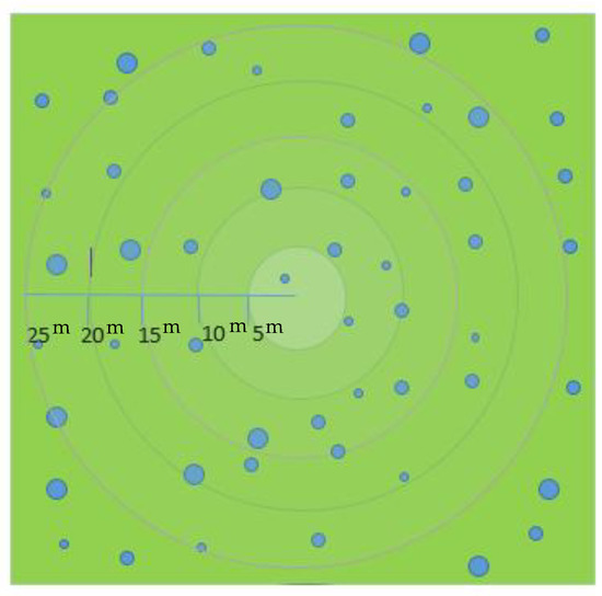
Figure 3.
Nested plot method.
We selected plots from the 118 plots in the study region where the dominant species was P. radiata (i.e., the percentage of P. radiata specimens was above 80%). Point clouds corresponding to the selected plots were compared with their corresponding orthophotos in order to detect differences that could interfere in the final result. We discarded plots where silvicultural treatments had decreased the population of P. radiata significantly, and plots with obvious mistakes in the point cloud classification. After this data cleansing, 55 plots remained (Figure 4).
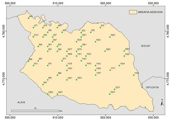
Figure 4.
Sample plots distribution of the National Forest Inventory 4 (NFI4) in Arratia-Nervión (ETRS89 UTM zone 30 North reference system).
The tree diameter at breast height (DBH mm) of the tree (1.3 m) was measured using a caliper in two perpendicular directions. The tree height (m) was determined by a hypsometer. These two measures are the independent variables of the allometric equations. In our data sample, the minimum, mean, and maximum values for the tree diameter and height are 10.5, 33.94, and 78.30 cm; and 4.30, 22.91, and 42.20 m, respectively (Figure 5).
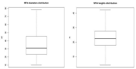
Figure 5.
Distribution of the diameter and height, respectively, of all the trees measured in the National Forest Inventory 4 (NFI4) that were taken into account for the estimation.
2.3. Field Plot Positioning
The positioning of the plots was carried out, according to the NFI4 specifications, with a GPS navigator obtaining autonomous observations without any differential correction. In order to study the effect of the plot positioning error, we have shifted the plot position by 10 m in each of the compass rose directions, obtaining eight new plots around the original one as shown in Figure 6. We assume that the plots are embedded in a homogeneous forest area, so that these shifts will have no effect.
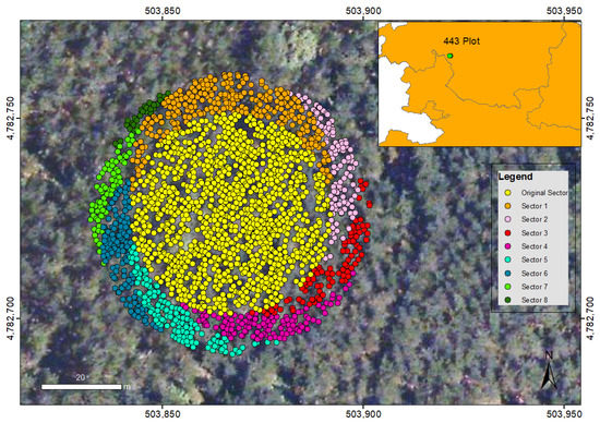
Figure 6.
Representation of the simulated translation of the plot 443. Each color represents the gathered LiDAR data for the mentioned nine plots (ETRS89 UTM zone 30 North reference system).
We apply the Cohen’s kappa concordance test measuring the agreement between two observers [29] to evaluate the similarity between the nine samples. In this case, we have nine “observers” corresponding to the 95% percentile of the height obtained from the shifted nine samples. These agreement values range from 0 to 1, where 1 implies that the compared metrics are identical, and 0 that there is no agreement.
2.4. LiDAR Data
The LiDAR data were acquired during the summer of 2012 between 12 July and 28 August. The entire Basque Autonomous Community area was flown over using a Lite Mapper 6800 Airborne Laser Scanner at an average altitude aboveground level and average speed of 1100 m and 67 m/s, respectively. The pulse repetition frequency was 100 kHz and the scan frequency was 70 kHz. The maximum scan angle was 60° with a beam divergence <0.5 mrad. The average point density was 0.5 points/m2. The spatial localization of the points was obtained with a precision <10 cm. The reference system is the European Terrestrial Reference System 89 (ETRS89) and the coordinate system is UTM for the thirtieth time zone. The dataset was divided into sheets of 2 × 2 km of extension, classified into eight classes: Unclassified, Ground, Low Vegetation, Medium Vegetation, High Vegetation, Building, Low Points, and Reserved. The data are publicly available at: ftp://ftp.geo.euskadi.eus/lidar/LIDAR_2012_ETRS89/LAS/.
2.5. Orthophotos
The flight campaign carried out by the Basque Government from 23 July to 28 August 2012 produced orthophotos with a spatial resolution of 25 cm/pixel, which were used to detect possible defects in the NFI4 data, and contradictions between NFI4 and LiDAR data. These orthophotos were downloaded from the Spatial Data Infrastructure (SDI) of the Basque Country Government from the following site: ftp://ftp.geo.euskadi.eus/cartografia/Cartografia_Basica/Ortofotos/ORTO_2012/Hojas_JPG/5000/.
2.6. Methods
2.6.1. Biomass Field Calculation
Volume per tree was calculated using an allometric model developed by the HAZI Foundation [30] based on the destructive sample of 732 P. radiata specimens extracted from locations distributed across the Basque region. The sample was carried out between the years 1990 and 2001. HAZI’s model uses the diameter at breast height (d mm) and total tree height (h m) as input variables (Equation (2)):
The resulting biomass value was corrected adding 4.04% of the obtained volume, in order to account for the tree branches and upper part of the trunk discarded for wood production reasons. This fixed correction quantity is specified per species, independent of the characteristics of the forest stand. The biomass of each sample plot was computed applying the allometric equation (Equation (2)) to the measured trees in the plot, adding them and computing the extrapolation to the size of control plot (25 m radius) using the expansion factor defined in Equation (1). Stand volume is obtained as the addition of the expanded values of the tree volumes of each plot.
2.6.2. LiDAR Data Processing and Overall Process
The complete LiDAR processing workflow is displayed in Figure 7a. In the initial step, the original LiDAR data (stored in LAS format files) were cleaned to identify and filter out suspected erroneous points. This is an important step, as these points can introduce errors in ensuing calculations. For this task, the altimetry value range of the point cloud was divided into equal size (15 m) intervals, counting the number of returns falling in each interval. Automatic detection of erroneous returns is based on the detection of empty layers between non-empty layers. We filtered out 0.06% of the total number of echoes. In the following steps we use the FUSION/LDV (LiDAR Data Viewer) (http://forsys.cfr.washington.edu/fusion/fusionlatest.html) free software. The next step was the selection of the points corresponding to the circular plots of 25 m radius considered in the NFI4, maintaining the dimensions of the control plots.
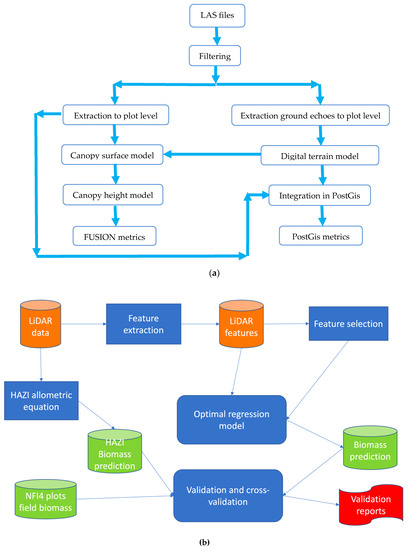
Figure 7.
(a) Flow chart of the Light Detection and Ranging LiDAR data. (b) Overall process carried out in the study.
The returns classified as ground were used to create a digital terrain model (DTM) with a spatial resolution of 1 m2/pixel. A digital surface model (DSM) was created with the highest returns of the point cloud over the sample plots, assigning the elevation of the highest return within each grid cell to the grid cell center. A canopy height model (CHM) was obtained by subtracting the DTM from the DSM. The CHM characterizes the tree canopy and it is able to give the canopy height directly. For each plot a large collection of metrics, that can be used as regressors for biomass prediction, was computed over all returns above a 2 m threshold [31,32], including height distributions, canopy density metrics, and descriptive statistics (these metrics are enumerated in Appendix A).
Canopy density metrics have demonstrated their usefulness as predictors of forest parameters such as mean height, dominant height, mean diameter, basal area, or timber volume [15]. We used the PostGis environment to obtain new metrics related to the canopy point density for each sample plot. The point cloud and the DTM were transformed into tables using routines developed with the PostGis spatial database extender for the PostgreSQL Database Management System. We divided the point cloud into 10 vertical layers of equal height. We set the lower limit at 2 m from the ground, to avoid shrubs, and the upper limit as the 95% percentile of the distribution of heights. This last metric was chosen instead of the maximum height, due to the stability demonstrated in previous studies [33,34]. Then, the routine counts the fraction of points falling inside each layer. That way, 10 canopy densities were computed (denoted as tr_1,..., tr_10).
Figure 7b provides a diagram describing the overall process carried out in the study. From the LiDAR data, we extract the LiDAR features that are the regressors of the regression model, we carry out a feature selection on the basis of the predictive performance and posthoc statistical tests of the regression model, selecting an optimal subset of LiDAR features. The NFI4 field data is used as the ground truth for model training and validation, which includes a cross-validation experiment as well as direct comparison of the predicted biomass with the NFI4 data for a site not included in the training data. Finally, we make additional comparison with the estimations provided by HAZI institute, which are produced by an allometric equation whose input variables are extracted from the LiDAR data.
2.6.3. Regression Analysis
This method computes a prediction of the variable under study as a linear combination of a set of regressor variables, often called features or input factors (Equation (3)):
Although it can be argued that the constant offset b0 does introduce a bias in the model, because setting all coefficients to zero would lead to a non-zero result, we are pretty sure that the specific context of the modeling in this paper does not include such degenerate case. We have extracted a large number of metrics from LiDAR data which can be used as regressors for biomass prediction. Some of them can be redundant or irrelevant. In order to select the most informative metrics to be used as regressors, firstly the Pearson correlation coefficient (r) was calculated between the biomass values and our LiDAR metrics. Secondly, the same operation was carried out between the logarithm of biomass values and our LiDAR metrics in order to check the linear relation. Dispersion graphics were used to ascertain the linear relation between the biomass and each of the candidate regressors.
Subsequently, we explored the quality of the prediction using all possible combinations of feature selections over the LiDAR metrics up to three variables per model. The adjusted coefficient of determination (R2adj) was used to assess the quality of the adjustment. R2adj represents the proportion of the variability explained by the adjusted model [35] after application of the correction factor described below. Additionally, standard error of the estimations (SEEs) were calculated in order to compare with other studies results. Akaike information criterion (AIC) is an index based on in-sample fit that can be used as an estimate of the likelihood of a model to predict the future values [36]. Our optimal feature selection corresponds to the model that has minimum AIC.
To check the hypothesis of the linear regression technique, several tests were applied to the trained models: Shapiro–Wilk test to verify the normality of the residuals, Breusch–Pagan test to analyze the homoscedasticity of the residuals, Durbin–Watson test to detect possible dependencies between the data, Variance Inflation Factor (VIF) to detect collinearity problems in the model [37], Ramsey´s RESET linearity test to verify lineal relations, and, finally, Bonferroni´s test to find statistically significant atypical values. All tests, except VIF, were calculated at the 95% level of significance.
When using the log model, it is necessary to compute the inverse of the logarithmic transformation, which may introduce some bias in the distribution of the estimated biomass values leading to under-estimation of the biomass [38]. To minimize the bias introduced in the model, a correction factor was applied, which depended on the standard error of the estimate (SEE). Once the SEE is calculated, the correction factor is computed as follows:
We carried out a sensitivity analysis of the model using an extended FAST (Fourier amplitude sensitivity test), because it is able to capture the influence of each regressor over its full range of variation. The objective of the sensitivity analysis (SA) of a regression model output is to ascertain how its output depends on its regressors [39]. This test allows the computation of the total contribution of each regressor to the variance of the output, as well as all the contribution of the interaction terms involving that regressor.
Let the fitted regression model be denoted as:
where Xi is a regressor model. The, Si is the contribution of regressor Xi to the variance of the output Y as specified in the following:
where E(Y|Xi) is the expectation of the output Y conditioned to input factor Xi and V(Y) the unconditional variance of the model output, which can be decomposed into the conditional regressor variances Vi.. as follows:
Dividing both sides of the equation above by V(Y) we obtain:
where Si is the first-order sensitivity index for regressor Xi, and Sij is the second-order sensitivity index for the interaction between regressors Xi and Xj with j≠i. The total contribution of regressor Xi to output Y variability is computed as follows:
STi is the total effect on the output variation due to factor Xi, adding its first-order effect and all higher-order effects due to interactions with other regressors. When the sum of the first-order index and total-effect index of a variable is not equal to one, interactions among factors in the model may occur. Additionally, we compute the fraction of the output variance arising from the uncertainty of each regressor Xi, and the complementary set of regressors, denoted D1 and Dt, respectively.
The biomass and the LiDAR data of one of the municipalities included in the study region, Orozko (Figure 8), was used to fit the LiDAR regression model. This municipality encompasses almost the 24% of the total population of P. radiata in the study area. More than 4260 ha of P. radiata were used for the model parameter estimation, taking into account all the polygons of the species located in the study area according to the NFI4 for the Basque Country and their occupation percentage. The biomass estimations provided by HAZI foundation for this municipality were used as the ground truth biomass. For its estimation, HAZI used NFI4 data and LiDAR data from the flight of 2012. They build a linear regression model of the wood volume using the mean height of the LiDAR points above 4 m aboveground as the single regressor of the model. Then, the biomass was calculated by adding, to the volume, 4% of the obtained volume, because when calculating the volume, the tree’s branches and a part of the trunk is not taken into account because of wood production reasons. This fixed quantity is stipulated per species, independent of the characteristics of the forest stand.
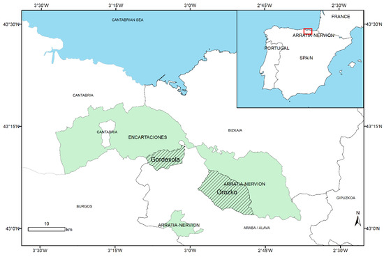
Figure 8.
Inset: Localization of the experiment area in Spain. Picture: Model application area shaded is Orozoko in Arratia-Nervión and model validation area is Gordexola in Encartaciones.
2.6.4. Validation
The validation process consists in the comparison between the biomass predictions and the observations over a set of measures that are different to the ones used in the model adjustment [40]. For this purpose, we used the data from Encartaciones region (Biscay) because of its large amount of P. radiata forests. This region is composed of eighteen municipalities, with a total area of 55,300 ha. Specifically, we use the data from the Gordexola municipality to validate the model because it includes almost 20% of the entire population of P. radiata of the region (Figure 15). More than 2600 ha of P. radiata were used to validate the model, according to the NFI4 polygons (Figure 8).
Besides, a k-fold cross-validation technique was applied with the same data that was used for the regressor selection, whereby the entire number of sample plots was divided into k = 10 subsamples composed of similar number of plots. The parameter estimation and validation was repeated k times, taking, each time, a different fold as the test and the remaining k-1 folds as the data for model training. The mean square error (MSE), was calculated as follows (Equation (10)):
where, lnYi is the natural logarithm of the values of the dependent variable, is the natural logarithm of the model estimations, N the number of cases of the sample. In fact, we will use the root of the MSE (RMSE) [41].
3. Results
3.1. Results
Firstly, we study positioning error effect, reporting the results of the Cohen concordance test. Table 1 shows the agreement between the original plot and the eight translated plots for plot 443 (the same procedure was applied to the remaining 54 plots). The agreement level among plots shown in the upper triangle of the matrix is close to 1, with a minimum value of 0.9. Hence, the eight plots created around the original one are similar enough to assure the low influence of the positioning error.

Table 1.
Cohen concordance test for plot 443. The concordance between the original plot (0) and the eight displaced plots according to the compass rose.
We computed the correlation matrix between the LiDAR data based regressors (specified in detail in Table A1) and the field biomass values and their logarithm. The highest correlated regressors were the height percentiles reaching maximal correlations of r = 0.80 and r = 0.86 with the biomass and the log-biomass, respectively. Although the regressors induced from canopy density measures were not highly correlated with the biomass, their relation to the biomass was statistically significant for all of them, reaching a maximum r = 0.62.
The linear relation can be assessed using dispersion diagrams in Figure 9 [42]. The shaded band is a pointwise 95% confidence interval on the fitted values (the blue line).
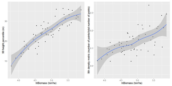
Figure 9.
Dispersion diagrams between the logarithm of the biomass and the most correlated height percentile and canopy density metric.
After the identification of the highest log-biomass correlated variables, and assessing their relationship, we fitted the best models using only one variable, two variables, or the combination of three variables.
The inclusion of three variables improved the adjusted coefficient of determination (R2adj = 0.81) in some cases, but introducing the third variable was not statistically significant in the models, hence, we discarded using more than two variables. Since the models presented in the table have very similar R2 values, further statistical analysis was undertaken to decide which model better fulfilled the assumptions of the linear regression analysis.
As can be seen in Table 2, the ten best fitting MLR models obtained very similar results in the inference tests. The models show identical numerical values for the R2adj value (0.79) and standard error (0.25 ton/ha in logarithmic units), the remaining columns reporting tests results had similar values too, including the detection of outliers according to Bonferroni´s test in all the models, where no outliers were detected. Regarding the normality of the residuals, it is not possible to reject this hypothesis in any model. The results are slightly better in the models using the 99% percentile of the height. In the case of the Breusch–Pagan test, the p-values values do not vary too much among regressor subsets, so it will be acceptable for all the models in the table, corresponding the best results (in the sense of non-rejection of null hypothesis) to the eighth model. The values obtained for the Durbin–Watson test and the variance inflation factor are very similar for all the models, concluding that no autocorrelation or collinearity problems were detected. The RESET linearity test results confirm the null hypothesis of a linear functional dependence of the biomass on the regressors for all tested models.
Table 2.
Accuracy values and test p-values obtained for the ten best models; p-values are shown for all the tests except VIF. p99, p95, and p90 are the 99%, 95%, and 90% percentiles of the laser canopy heights, respectively; tr_2, tr_3, and tr_4 are the canopy densities corresponding to the second, third, and fourth layers, respectively; allabovemean = (all returns above mean height)/(total returns). R2adj = adjusted coefficient of determination; SE = Standard Error; AIC = Akaike information criterion; SW = Shapiro-Wilk residuals normality test; BP = Breustch–Pagan residuals homoscedasticity test; DW = residuals autocorrelationi test; VIF = Variance Inflation Factor; reset = Ramsey´s RESET linearity test; B = Bonferroni outlier test.
For the optimal selection of variables, we focus on the Breusch–Pagan test as heteroscedasticity is to be avoided in regression models, thus the selected model is {p95, tr_3} (i.e., the one composed of the 95% percentile of the LiDAR measurement of canopy heights (p95), and the percentage of points above the third layer from the total number of returns (tr_3)). The equation corresponding to this model is the following (Equation (11)):
As it has been commented in Section 2.6.3, the logarithmic values of the estimated biomass must be transformed to arithmetic values. In this case the value obtained for the correction factor was 1.032, hence, the biomass equation reads:
Extensive diagnostic graphics, shown in Figure 10, Figure 11 and Figure 12, were carried out on the best model. It does not show heteroscedasticity behavior, as it can be checked upon inspection of the “residual vs. fitted” values plot, and the “Scale Location” plot, where no tendency of the residuals can be identified. The Quantile-Quantile (Q-Q) plot confirms the normality assumption of the residuals, previously checked by a Shapiro–Wilks test. There are “light tails” in the Q-Q plot, more pronounced in the right side of the plot, so it is detecting that there were more extreme values than would be expected for a truly normal distribution. The results of the Bonferroni test already removed doubts over the existence of outliers or atypical values. The dispersion plots in Figure 11 and Figure 12 confirm the linear dependency hypothesis, and the normality of the residuals of the model predictions.
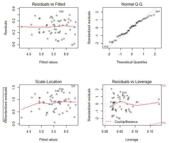
Figure 10.
Extensive diagnostics graphics for the chosen model, being Normal Q-Q the Quantile-Quantile plot.
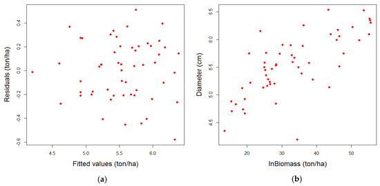
Figure 11.
(a) Dispersion diagram between residuals and the fitted values of the logarithm of the biomass; and (b) dispersion diagram between the diameter and the logarithm of the biomass in field.
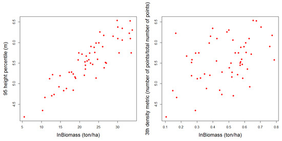
Figure 12.
Dispersion diagrams between the two regressors of the chosen model and the logarithm of the biomass.
The minimum, mean, and the maximum estimated biomass per plot was 69.06, 294.77, and 611.21 ton/ha, respectively. As can be shown in Figure 13, the distribution of the biomass estimations does not appear to be normal. We visualize in Figure 14 the spatial location of the sample plots and the magnitude of the biomass estimated at each plot.
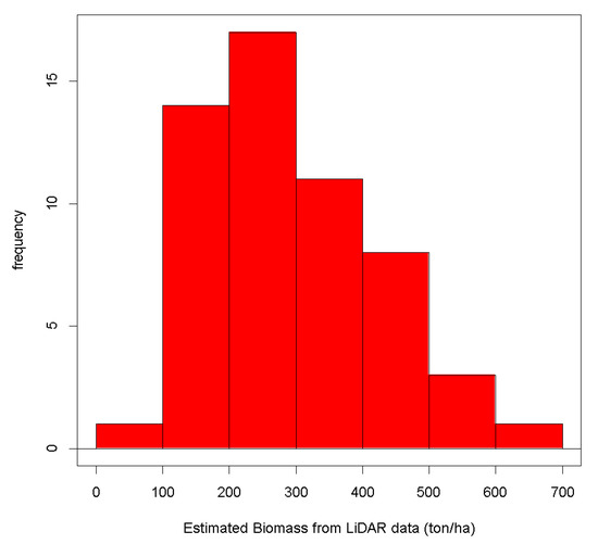
Figure 13.
Distribution of the biomass estimations computed by the LiDAR regression model.
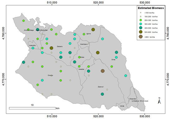
Figure 14.
Visualization of the biomass estimation at each of the 55 sample plots.
We carry out statistical inference over the linear regression model with optimal regressor selection obtaining the upper and lower bounds shown in Table 3. The average biomass estimate over the 55 sample plots is 294.77 ton/ha. Its lower and upper bounds of the 95% confidence interval are 189.79 and 460.37 ton/ha, respectively.
Table 3.
The 95% confidence level inference over the model coefficient values.
The average inference over the biomass estimated in the 55 plots is 294.77 ton/ha, establishing as low and upper limit at a 95% confidence interval, 189.79 and 459.05 ton/ha, respectively.
In addition to these values, simulations in each of the 55 plots were performed, doing 10,000,000 iterations in each plot, at a 95% confidence interval applying Monte Carlo simulation. Monte Carlo uses random samples to simulate data for a certain mathematical model. The results were very similar to the ones previously obtained, in this case, the average value of the biomass is exactly the same and the low and upper limit are 190.35 and 460.37 ton/ha respectively.
Sensitivity analysis with the extended FAST test [43] was carried out, using M = 4 as interference factor and n = 17 as sample size. The results of the analysis are displayed in Table 4. The model appeared to be non-additive because the sum of the first-order index and the total-effect index is not equal to one for both regressors. Hence, there must be interactions among them. The existence of interactions may imply, for instance, that extreme values of the output Y are uniquely associated with particular combinations of model inputs, in a way that is not described by the first-order effects (Si). The total-effect indices (STi) show that only p95 is taking part in the interactions, because STi > Si. D1 represents the portion of the output variance arising from the uncertainty of factor i, while DT is the variance for the complementary set D(-i) [44]. First-order effect (Si) is bigger for the density metric than for the percentile of the height, which implies that this variable is more sensible in the model. D1 and DT corroborates this tendency, pointing that the density metric contributes more than the height percentile to the output variance, because D1 is bigger for the density metric than for the height percentile.
Table 4.
Sensitivity analysis results. Si = first-order effects; STi = total-effect index; D1 = the portion of the output variance arising from the uncertainty of factor i; DT = variance for the complementary set D(-i).
3.2. Application of the Selected Model
The fitted optimal regression model was applied to LiDAR data extracted from the Orozko municipality, in Arratia-Nervión, comparing its biomass estimation with the biomass estimation given by the HAZI foundation using allometric equations applied to field measurements, finding a difference of 8%, 992,747.53 vs. 915,851.29 ton. The spatial distribution of the estimation of our regression model is visualized in Figure 15.
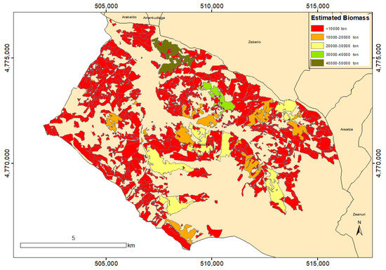
Figure 15.
Biomass estimations for Orozko municipality (Arratia-Nervión) by the application of the developed model.
3.3. Validation of the Selected Model
As detailed in Section 2.6.4, the first validation step applied the developed model in the Gordexola municipality (an independent area). A difference of 121,734.65 ton was obtained between the biomass given by the HAZI foundation (561,868.93 ton) and the one estimated in this study (683,603.58 ton), representing approximately 21% of the total biomass of the Gordexola municipality.
In a second step, a k-fold cross-validation was also applied, in which the initial sample, composed of the same 55 plots used to estimate the model, was subdivided in five equal folds and the algorithm fitted to the model using the k-1 remaining folds. Eleven elements were used per fold, with the mean value of the addition of the square of the residuals oscillating between 0.0674 and 0.0682 logarithmic units, more or less 0.7% of the mean value of the field biomass, suggesting that the prediction values made were quite accurate.
4. Discussion
We proposed and tested a linear regression model of the logarithm of the biomass using regressors extracted from low point density LiDAR data. A ground truth biomass estimate was constructed by the application of an allometric model with dasometric values from the NFI4. Our optimal model has only two independent variables: a height percentile and a canopy density metric, both obtained from the LiDAR data. The model explains 80% of the variance of the sample with an RMSE of 0.5 in logarithmic units. Our results presented here are within the range of those reported by similar studies using LiDAR technology to characterize AGB in coniferous forest, profiting from higher density sampling LiDAR data [32,45,46,47]. Similar results to ours (R2 = 0.74; SE = 0.2) were reported by Hall et al. [48] in an area in Colorado, USA, for Pinus ponderosa and Pseudotsuga menziesii species. The density points in the American study were higher than the one used in our study (1.23 points/m2), but in their study the only variable introduced in the exponential model was a density metric, no metrics derived for the tree height were included.
Næsset and Gobakken [32] obtained higher R2 values (0.88) than us with a very similar value for RMSE (0.25 in logarithmic units) in a Norwegian area composed primarily of Pinus sylvestris and Picea abies using a point density up to 1.2 points/m2. Their chosen regressors were a high percentile of the LiDAR measured tree height (90% percentile) and a low-density metric. The density metric was more statistically significant in the Norwegian model than in our study: They found that the partial value of R2 for each variable was 0.61 and 0.21, respectively, while in our study the values were 0.74 and 0.15, respectively. The mean value of the estimated biomass was similar in both studies (150 ton/ha). Hence, differences in the model determination coefficient can be due to the geographical location, altitude, species composition, or site quality. Another relevant study [49] was carried out over the Taita Hills (55,000 ha), in southeast Kenya, with a pulse density of 3.1 points/m2. They used a boosted regression trees (BRT) technique for identifying regressors that better explain biomass distribution. Multilinear regression was used to predict aboveground biomass using LiDAR metrics (R2 = 0.88 and RMSE = 52.9 Mg/ha) and the mean AGB was 123 ton/ha. In this case, the point density was significantly higher than in our study. It has been shown that pulse density below 1 pulse/m2 has a negative influence on the quality of the prediction [50].
The results obtained by González-Ferrreiro et al. [46] for P. radiata in Galicia (Spain) were very similar to ours (R2 = 0.74, RMSE = 40.469 ton/ha). The study area was situated in the north of the peninsula too, with similar conditions to those found in the Arratia-Nervión (mean biomass = 150 ton/ha in both cases), but their point density was very high (8 points/m2). In the province of Zaragoza (Spain), the work reported in [26] estimated the biomass with good results (R2 = 0.89, RMSE = 7326.12 kg/ha), but the mean and the maximum biomass measured in the field were much lower, along with the variability of the samples.
The Q-Q plot in Figure 10 corroborates the normality of the residuals, but moderate tails can be appreciated, which are slightly heavier in the right side of the figure. This shows that the normality of the residuals decreases when their values increase, which translates into biomass underestimation in relation with the field measurements. The plots with higher errors (>40%) correspond to the same timber stage, with tree diameters higher than 20 cm. Even the residuals do not show a clear tendency, indicating an overestimation between LiDAR heights and those measured in the field (max. 10 m), when the opposite was expected due to the difficulty of the LiDAR to detect the top of the trees [42]. These differences might be related with errors during the field data acquisition, the time mismatch between both data sets, and, finally, errors in the height determination from the LiDAR data. Apart from these circumstances, the usage of the circular nested-plots methodology applied in the NFI4 and the extrapolation of the data to the 25 m plot may be another source of error. No observation has exceeded the Cook distance in the “residual vs. leverage” plot, so they might not be influential observations, but it is true that some observations had high residuals.
No homoscedasticity issues were detected in the model, when the adjusted values of biomass were compared graphically with the residuals (Figure 11a), hence, it can be concluded that the variance of the residual is independent of the regressors. Furthermore, the linear adjustment seems to be the most suitable, as the linearity test confirmed. A clear relationship exists between the diameter measured in field and the estimated biomass (Figure 11b), as the values of the biomass increase, the values of the diameter are more disperse. This condition is well known in the use of statistics models for biological phenomena where high variability can appear: Equal dimensions of the trunk does not imply equal quantity of biomass, because it depends on the growing conditions of the trees [14]. As can be seen in Figure 12, the linear relationship between the logarithm of the biomass and the 95% height percentile is more evident than the relation between the explicated variable and the canopy density metric included in the model. As the regression proves, the p-value obtained was <0.001 for the percentile, and 0.039 for the density metric regressor, with a significance level of 0.05. But no other tendencies were deduced from the plots.
The main motivation of our study is to show that LiDAR data with lower point density than the densities reported in LiDAR data capture missions dedicated to biomass measurement can be used for AGB estimation. In this regard, some studies have estimated biomass using data with low point densities obtained by subsampling LiDAR data from flights especially designed for biomass estimation studies, with the aim of analyzing the influence of point densities in the final estimations. Authors report different conclusions. One study calculated the biomass in a forested area of central Spain, using LiDAR data with a final average point density of 11.4 points/m2, due to the acquisition of several overlapped scans [51]. They report results from nine different point density values: 0.25, 0.5, 1, 1.5, 2, 3, 4, 5, and 6 points/m2, obtaining increasing values for R2 ranging from 0.69 to 0.92 as the point density increased. Another work [52] analyzed the importance of the point density for biomass estimation in three different sites across Ontario, Canada. They concluded that even with a very low point density of 1/100, automated LiDAR scan (ALS) is a feasible option for assessing AGB in vast areas of flat, lowland peat swamp forest. Additionally it has been found [50] that the accuracy of predicted forest structure metrics decreases as the pulse density decreases, remaining relatively high until low densities (e.g., 1 pulse/m2). Due to the influence of all these factors, replication effects can be detected in the final AGB estimations. Magnussen et al. [53] found that a minimum point density of 1 point/m2 was needed to reduce the replication variance in LiDAR-derived predictions. Known factors affecting extracted ALS-based predictors of forest inventory attributes are instrument errors, positional errors, and posts-capture data-processing errors. We must take into account that these factors limit the ability to replicate results of AGB estimation. However, the major conclusion of the reviewed studies is that useful AGB estimations can be obtained from low-density LiDAR data, as done in our study.
The difference obtained between the biomass estimation data provided by the HAZI foundation and our predictions may be due to the combination of various uncontrollable sources of variability along the data extraction and computational processes. Firstly, HAZI calculated the wood volume using the allometric equation applied to tree measures extracted from LiDAR data, while we estimated the biomass directly from the LiDAR data, avoiding the accumulation of errors due to the concatenation of various mathematical processes. HAZI subsequently added, to the estimated volume, a constant percentage of the obtained volume, which is species specific. Corona et al. [54] have derived a ratio estimator of the total volume of a forest, constituting an approximately unbiased estimator of the total volume of its sampling variance and the corresponding confidence interval. This method needs a very accurate georeference and co-registration of both LiDAR measurements and plot locations. In addition, in large areas, including forest stands with different characteristics (species, silvicultural treatments, age structures, etc.), stratification will be required.
Even if the developed biomass estimation model is local, the designed automatic and straightforward process to obtain the biomass estimations can be applied in different regions and for different species. The main limitation of the application of the explained methodology is the availability of public LiDAR and National Forest Inventory (NFI4) data. The LiDAR data used in this study are publicly available, continuous in time, and are collected in cycles of four/five years, more frequently than the data gathered in the NFI4. This study found that height percentiles were the most relevant height-related regressors for biomass prediction. As other authors have found [55], canopy density metrics have statistical significance in the model and, hence, were included. There are some major sources of unexplained variance of the AGB regression model [56,57,58]). The first is mis-registration of the ground plot locations to the LiDAR point cloud. As has been shown above, position errors are not influential in the results. The second is the application of allometric equations for biomass predictions over the ground measurements. In the NFI4 not all of the trees were measured, as we have explained, only some individuals were measured and then the values were extrapolated. The third error source would be related with the plot size, because of the disagreement between LIDAR and field plot measurements, over which trees or parts of trees are inside calibration plots. The biomass estimations presented in this study may be influenced by the exclusion in the ground data of overhanging tree crowns captured by LiDAR, which may lead to underestimation of the final result [8]. Finally, classification errors of the LiDAR data into levels could interfere with the results. Carrying out information fusion with other sensors [59,60] may alleviate these problems
According to the quality curves 1, 2, and 3 for P. radiata species for the Basque Country developed in 1974, the estimated average growth per year is approximately 1 m. In the adjusted regression models, our regressors are the LiDAR heights from the flight of 2012, while our ground truth is the biomass measured in 2011, thus we have only one year of growth to account for. In the ground truth volume measurements, a correction of 4% was added to account for biomass discarded by the field researchers. We believe that the one-year growth missed can be accounted for by this operation.
5. Conclusions
This study has shown the application of an automatic and straightforward process to develop a local model to estimate biomass of P. radiata using LiDAR data from a low point density flight (0.5 points/m2). The approach could be transferred to other areas, if LiDAR and forest inventory datasets are available, and could become a powerful tool for complimenting other traditional methods (e.g., NFI4), reducing significantly the high investment of time and money required by such methodologies.
Based on the encouraging results obtained in this study, we will propose machine learning techniques to improve results in future studies. Similarly, the incorporation of data from additional sensors (e.g., hyperspectral images or synthetic aperture radar) could help improve the model-based results. For future research, exploiting open data from the European Copernicus program could be a good avenue to obtain improved predictive models comprising satellite-borne Earth observation and in-situ data. A service component that combines these information sources will provide essential information for monitoring the terrestrial environment.
Author Contributions
Conceptualization L.T.T. and J.M.S.E.; methodology L.T.T. and J.M.S.E. All Authors contributed to the interpretation of the results and to the discussion, to the original draft preparation and to the review process.
Funding
The work reported in this paper was partially supported by FEDER funds for the MINECO project TIN2017-85827-P, and project KK-2018/00071 of the Elkartek 2018 funding program of the Basque Government. Additional support comes from grant IT1284-19 of the Basque Country.
Acknowledgments
The authors are grateful to the University of the Basque Country and the University of Cantabria for providing technical and personal resources for this research. We would like to thank the Spanish National Forest Inventory for collecting the field data, the Basque Government for the acquisition, processing, and publication of the LiDAR data, and staff of the HAZI foundation for their availability and excellent response.
Conflicts of Interest
The authors declare no conflict of interest.
Appendix A
Table A1.
Metrics collection obtained with FUSION.
Table A1.
Metrics collection obtained with FUSION.
| Variable | Description | Variable | Description |
|---|---|---|---|
| count | number of returns above the minimum height | ccr | canopy relief ratio:((mean - min)/(max – min) |
| densitytotal | total returns used for calculating cover | eqm | elevation quadratic mean |
| densityabove | returns above height break | ecm | elevation cubic mean |
| densitycell | density of returns used for calculating cover | r1count,…,r9count | count of return 1,…,9 points above the minimum height |
| min | minimum value for cell | rothercount | count of other returns above the minimum height |
| max | maximum value for cell | allcover | (all returns above cover height (h))/(total returns) |
| mean | mean value for cell | afcover | (all returns above cover h)/(total first returns) |
| mode | modal value for cell | allcount | number of returns above cover h |
| stddev | standard deviation of cell values | allabovemean | (all returns above mean h)/(total returns) |
| variance | variance of cell values | allabovemode | (all returns above h mode)/(total returns) |
| cv | coefficient of variation for cell | afabovemean | (all returns above mean h)/(total first returns) |
| cover | cover estimate for cell | afabovemode | (all returns above h mode)/(total first returns) |
| abovemean | proportion of first (or all) returns above the mean | fcountmean | number of first returns above mean h |
| abovemode | proportion of first (or all) returns above the mode | fcountmode | number of first returns above h mode |
| skewness | skewness computed for cell | allcountmean | number of returns above mean h |
| kurtosis | kurtosis computed for cell | allcountmode | number of returns above h mode |
| AAD | average absolute deviation from mean for the cell | totalfirst | total number of first returns |
| p01,…,p99 | 1st,…,99th percentile value for cell | totalall | total number of returns |
| iq | 75th percentile minus 25th percentile for cell |
References
- IPCC. Climate Change 2014: Synthesis Report. Contribution of Working Groups I, II and III to the Fifth Assessment Report of the Intergovernmental Panel on Climate Change; Core Writing Team, Pachauri, R.K., Meyer, L.A., Eds.; IPCC: Geneva, Switzerland, 2014; 151p. [Google Scholar]
- Poudel, K.P.; Temesgen, H. Methods for estimating aboveground biomass and its components for Douglas-fir and lodgepole pine trees. Can. J. For. Res. 2016, 46, 77–87. [Google Scholar] [CrossRef]
- Bi, H.; Long, Y.; Turner, J.; Lei, Y.; Snowdon, P.; Li, Y.; Harper, R.; Zerihun, A.; Ximenes, F. Additive prediction of aboveground biomass for Pinus radiata (D. Don) plantations. For. Ecol. Manag. 2010, 259, 2301–2314. [Google Scholar] [CrossRef]
- Espinosa, M.; Acuña, E.; Cancino, J.; Perry, D.A. Carbon Sink Potential of Radiata Pine Plantations in Chile. Forestry 2005, 78, 11–19. [Google Scholar] [CrossRef]
- Aragonés, A.; Espinel, S.; Ritter, E. Caracterización mediante el uso de RADP de la población de Pinus radiata del País Vasco. Invest. Agr. Sist. Rec. For. 1994, 3, 135–146. [Google Scholar]
- Cuarto Inventario Forestal Nacional COMUNIDAD AUTÓNOMA DEL PAÍS VASCO/EUSKADI.
- Corona, P. Consolidating new paradigms in large-scale monitoring and assessment of forest ecosystems. Environ. Res. 2016, 144, 8–14. [Google Scholar] [CrossRef] [PubMed]
- Corona, P. Integration of forest mapping and inventory to support forest management. iForest 2010, 3, 59–64. [Google Scholar] [CrossRef]
- Guo, Z.; Chi, H.; Sun, G. Estimating Forest Aboveground Biomass using HJ-1 Satellite CCD and ICESat GLAS Waveform Data. Sci. China-Earth Sci. 2010, 53, 16–25. [Google Scholar] [CrossRef]
- Næsset, E.; Gobakken, T.; Solberg, S.; Gregoire, T.G.; Nelson, R.; Ståhl, G.; Weydahl, D. Model-Assisted Regional Forest Biomass Estimation using LiDAR and InSAR as Auxiliary Data: A Case Study from a Boreal Forest Area. Remote Sens. Environ. 2011, 115, 3599–3614. [Google Scholar] [CrossRef]
- Nelson, R.; Margolis, H.; Montesano, P.; Sun, G.; Cook, B.; Corp, L.; Andersen, H.; deJong, B.; Pellat, F.P.; Fickel, T.; et al. Lidar-Based Estimates of Aboveground Biomass in the Continental US and Mexico using Ground, Airborne, and Satellite Observations. Remote Sens. Environ. 2017, 188, 127–140. [Google Scholar] [CrossRef]
- García, M.; Saatchi, S.; Ustin, S.; Balzter, H. Modelling Forest Canopy Height by Integrating Airborne LiDAR Samples with Satellite Radar and Multispectral Imagery. Int. J. Appl. Earth Observ. Geoinf. 2018, 66, 159–173. [Google Scholar] [CrossRef]
- Nelson, R.; Oderwald, R.; Gregoire, T.G. Separating the ground and airborne laser sampling phases to estimate tropical forest basal area, volume, and biomass. Remote Sens. Environ. 1997, 60, 311–326. [Google Scholar] [CrossRef]
- Nilsson, M. Estimation of tree heights and stand volume using an airborne lidar system. Remote Sens. Environ. 1996, 56, 1–7. [Google Scholar] [CrossRef]
- Næsset, E. Predicting forest stand characteristics with airborne scanning laser using a practical two-stage procedure and field data. Remote Sens. Environ. 2002, 80, 88–99. [Google Scholar] [CrossRef]
- Shi, Y.; Wang, T.; Skidmore, A.K.; Heurich, M. Important LiDAR Metrics for Discriminating Forest Tree Species in Central Europe. ISPRS J. Photogramm. Remote Sens. 2018, 137, 163–174. [Google Scholar] [CrossRef]
- Vaglio Laurin, G.; Puletti, N.; Chen, Q.; Corona, P.; Papale, D.; Valentini, R. Above Ground Biomass and Tree Species Richness Estimation with Airborne Lidar in Tropical Ghana Forests. Int. J. Appl. Earth Observ. Geoinf. 2016, 52, 371–379. [Google Scholar] [CrossRef]
- Magnussen, S.; Nord-Larsen, T.; Riis-Nielsen, T. Lidar Supported Estimators of Wood Volume and Aboveground Biomass from the Danish National Forest Inventory (2012–2016). Remote Sens. Environ. 2018, 211, 146–153. [Google Scholar] [CrossRef]
- Ene, L.T.; Gobakken, T.; Andersen, H.; Næsset, E.; Cook, B.D.; Morton, D.C.; Babcock, C.; Nelson, R. Large-Area Hybrid Estimation of Aboveground Biomass in Interior Alaska using Airborne Laser Scanning Data. Remote Sens. Environ. 2018, 204, 741–755. [Google Scholar] [CrossRef]
- Shao, G.; Shao, G.; Gallion, J.; Saunders, M.R.; Frankenberger, J.R.; Songlin, F. Improving Lidar-based aboveground biomass estimation of temperate hardwood forests with varying site productivity. Remote Sens. Environ. 2018, 204, 872–882. [Google Scholar] [CrossRef]
- Nelson, R.; Krabill, W.; MacLean, G. Determining Forest Canopy Characteristics using Airborne Laser Data. Remote Sens. Environ. 1984, 15, 201–212. [Google Scholar] [CrossRef]
- Popescu, S.C. Estimating Biomass of Individual Pine Trees using Airborne Lidar. Biomass Bioenergy 2007, 31, 646–655. [Google Scholar] [CrossRef]
- Goldbergs, G.; Levick, S.R.; Lawes, M.; Edwards, A. Hierarchical Integration of Individual Tree and Area-Based Approaches for Savanna Biomass Uncertainty Estimation from Airborne LiDAR. Remote Sens. Environ. 2018, 205, 141–150. [Google Scholar] [CrossRef]
- Yavaşlı, D.D. Estimation of Above Ground Forest Biomass at Muğla using ICESat/GLAS and Landsat Data. Remote Sens. Appl. Soc. Environ. 2016, 4, 211–218. [Google Scholar] [CrossRef]
- Nie, S.; Wang, C.; Zeng, H.; Xi, X.; Li, G. Above-Ground Biomass Estimation using Airborne Discrete-Return and Full-Waveform LiDAR Data in a Coniferous Forest. Ecol. Indic. 2017, 78, 221–228. [Google Scholar] [CrossRef]
- Montealegre, A.L.; Lamelas, M.T.; de la Riva, J.; García-Martín, A.; Escribano, F. Cartografía De La Biomasa Aérea Total En Masas De Pinus Halepensis Mill. En El Entorno De Zaragoza Mediante Datos LiDAR-PNOA y Trabajo De Campo. Análisis espacial y representación geográfica: Innovación y aplicación; Universidad de Zaragoza: Zaragoza, Spain, 2015; pp. 769–776. [Google Scholar]
- I.C.O.N.A. Segundo Inventario Forestal Nacional. Explicaciones y Métodos, Spain, 1986–1995, 1990.
- Pearson, T.R.H.; Walker, S.; Brown, S. Sourcebook for Land Use, Land-Use Change and Forestry Projects; World Bank: Washington, DC, USA, 2005. [Google Scholar]
- Cohen, J. A Coefficient of Agreement for Nominal scales. Educ. Psychol. Measur. 1960, 20, 37–46. [Google Scholar] [CrossRef]
- Ecuaciones de cubicación para el pino radiata en el País Vasco – IKT/HAZI – Arkaute, Spain. 2004.
- Gobakken, T.; Næsset, E.; Nelson, R.; Bollandsås, O.M.; Gregoire, T.G.; Ståhl, G.; Holm, S.; Ørka, H.O.; Astrup, R. Estimating biomass in Hedmark County, Norway using national forest inventory field plots and airborne laser scanning. Remote Sens. Environ. 2012, 123, 443–456. [Google Scholar] [CrossRef]
- Næsset, E.; Gobakken, T. Estimation of Above- and Below-Ground Biomass across Regions of the Boreal Forest Zone using Airborne Laser. Remote Sens. Environ. 2008, 112, 3079–3090. [Google Scholar] [CrossRef]
- Næsset, E. Effects of Different Flying Altitudes on Biophysical Stand Properties Estimated from Canopy Height and Density Measured with a Small-Footprint Airborne Scanning Laser. Remote Sens. Environ. 2004, 91, 243–255. [Google Scholar] [CrossRef]
- Næsset, E.; Gobakken, T. Estimating Forest Growth using Canopy Metrics Derived from Airborne Laser Scanner Data. Remote Sens. Environ. 2005, 96, 453–465. [Google Scholar] [CrossRef]
- Walpole, R.E.; Myers, R.H.; Myers, S.L.; Ye, K. Probabilidad y Estadística Para Ingeniería y Ciencias; Novena, Ed.; Pearson Educational: Mexico D.F., Mexico, 2012. [Google Scholar]
- Akaike, H. A new look at the statistical model identification. IEEE Trans. Automat. Control 1974, 19, 716–723. [Google Scholar] [CrossRef]
- Kleinbaum, D.; Kupper, L.; Nizam, A.; Rosenberg, E. Applied Regression Analysis and Other Multivariable Methods, 5th ed.; Cengage Learning: Boston, MA, USA, 2014. [Google Scholar]
- Baskerville, G. Use of Logarithmic Regression in the Estimation of Plant Biomass. Can. J. Forest. Res. 1972, 2, 49–53. [Google Scholar] [CrossRef]
- Saltelli, A.; Ratto, M.; Campolongo, F.; Cariboni, J.; Gatelli, D.; Saisana, M.; Tarantola, S. Global Sensitivity Analysis; The Primer: West Sussex, UK, 2008. [Google Scholar]
- Rykiel, E.J., Jr. Testing Ecological Models: The Meaning of Validation. Ecol. Model. 1996, 90, 229–244. [Google Scholar] [CrossRef]
- Steel, R.G.D.; Torrie, J.H. Principles and Procedures of Statistics, with Special Reference to Biological Sciences; McGraw-Hill: New York, NY, USA, 1960. [Google Scholar]
- Picard, N.; Saint-André, L.; Henry, M. Manual for Building Tree Volume and Biomass Allometric Equations:Fromfiled Measurement to Prediction; Food and Agricultural Organization of the United Nations; Rome and Centre Coopération Internationale en Food and Agricultural Organization of the United Nations: Montpellier, France, 2012; 215p. [Google Scholar]
- Saltelli, A.; Tarantola, S.; Chan, K. A Quantitative, Model Independent Method for Global Sensitivity Analysis of Model Output. Technometrics 1999, 41, 39–56. [Google Scholar] [CrossRef]
- Homma, T.; Saltelli, A. Importance Measures in Global Sensitivity Analysis of Nonlinear Models. Reliabil. Eng. Syst. Saf. 1996, 52, 1–17. [Google Scholar] [CrossRef]
- Næsset, E. Estimating Above-Ground Biomass in Young Forests with Airborne Laser Scanning. Int. J. Remote Sens. 2011, 32, 473. [Google Scholar] [CrossRef]
- González-Ferreiro, E.; Aranda, U.; Miranda, D. Estimation of Stand Variables in Pinus Radiata D. Don Plantations using Different LiDAR Pulse Densities. Forestry 2012, 85. [Google Scholar] [CrossRef]
- He, Q.; Chen, E.; An, R.; Li, Y. Above-Ground Biomass and Biomass Components Estimation using LiDAR Data in a Coniferous Forest. Forests 2013, 4, 984–1002. [Google Scholar] [CrossRef]
- Hall, S.A.; Burke, I.C.; Box, D.O.; Kaufmann, M.R.; Stoker, J.M. Estimating Stand Structure using Discrete-Return Lidar: An Example from Low Density, Fire Prone Ponderosa Pine Forests. For. Ecol. Manag. 2005, 208, 189–209. [Google Scholar] [CrossRef]
- Adhikari, H.; Heiskanen, J.; Siljander, M.; Maeda, E.; Heikinheimo, V.; Pellikka, P.K.E. Determinants of Aboveground Biomass Across an Afromontane Landscape Mosaic in Kenya. Remote Sens. 2017, 9, 1–19. [Google Scholar] [CrossRef]
- Jakubowski, M.K.; Guo, Q.; Kelly, M. Tradeoffs between lidar pulse density and forest measurement accuracy. Remote Sens. 2013, 130, 245–253. [Google Scholar] [CrossRef]
- Ruiz, L.A.; Hermosilla, T.; Mauro, F.; Godino, M. Analysis of the Influence of Plot Size and LiDAR Density on Forest Structure Attribute Estimates. Forests 2014, 5, 936–951. [Google Scholar] [CrossRef]
- Treitz, P.; Lim, K.; Woods, M.; Pitt, D.; Nesbitt, D.; Etheridge, D. LiDAR Sampling Density for Forest Resource Inventories in Ontario, Canada. Remote Sens. 2012, 4, 830–848. [Google Scholar] [CrossRef]
- Magnussen, S.; Næsset, E.; Gobakken, T. Reliability of LiDAR Derived Predictors of Forest Inventory Attributes: A Case Study with Norway Spruce. Remote Sens. Environ. 2010, 114, 700–712. [Google Scholar] [CrossRef]
- Corona, P.; Fattorini, L. Area-based lidar-assisted estimation of forest standing volume. Can. J. For. Res. 2008, 38, 2911–2916. [Google Scholar] [CrossRef]
- Næsset, E.; Gobakken, T.; Bollandsås, O.M.; Gregoire, T.G.; Nelson, R.; Ståhl, G. Comparison of Precision of Biomass Estimates in Regional Field Sample Surveys and Airborne LiDAR-Assisted Surveys in Hedmark County, Norway. Remote Sens. Environ. 2013, 130, 108–120. [Google Scholar] [CrossRef]
- D'Oliveira, M.V.N.; Reutebuch, S.E.; McGaughey, R.J.; Andersen, H. Estimating Forest Biomass and Identifying Low-Intensity Logging Areas using Airborne Scanning Lidar in Antimary State Forest, Acre State, Western Brazilian Amazon. Remote Sens. Environ. 2012, 124, 479–491. [Google Scholar] [CrossRef]
- Mascaro, J.; Detto, M.; Asner, G.P.; Muller-Landau, H.C. Evaluating Uncertainty in Mapping Forest Carbon with Airborne LiDAR. Remote Sens. Environ. 2011, 115, 3770–3774. [Google Scholar] [CrossRef]
- García-Gutiérrez, J.; Martínez-Álvarez, F.; Troncoso, A.; Riquelme, J.C. A Comparison of Machine Learning Regression Techniques for LiDAR-Derived Estimation of Forest Variables. Neurocomputing 2015, 167, 24–33. [Google Scholar] [CrossRef]
- Vaglio Laurin, G.; Chen, Q.; Lindsell, J.A.; Coomes, D.A.; Frate, F.D.; Guerriero, L.; Pirotti, F.; Valentini, R. Above Ground Biomass Estimation in an African Tropical Forest with Lidar and Hyperspectral Data. ISPRS J. Photogramm. 2014, 89, 49–58. [Google Scholar] [CrossRef]
- Treuhaft, R.N.; Anser, G.P.; Law, B.E. Structure-Based Forest Biomass from Fusion of Radar and Hyperspectral Observations. Geophys. Res. Lett. 2003, 30, 1472–1487. [Google Scholar] [CrossRef]
© 2019 by the authors. Licensee MDPI, Basel, Switzerland. This article is an open access article distributed under the terms and conditions of the Creative Commons Attribution (CC BY) license (http://creativecommons.org/licenses/by/4.0/).