Article

Temporal Evolution of Carbon Stocks, Fluxes and Carbon Balance in Pedunculate Oak Chronosequence under Close-To-Nature Forest Management

by
Maša Zorana Ostrogović Sever
1,
Giorgio Alberti
2,3,
Gemini Delle Vedove
2 and
Hrvoje Marjanović
1,*
1
Department of Forest Management and Forestry Economics, Croatian Forest Research Institute, Cvjetno naselje 41, 10450 Jastrebarsko, Croatia
2
Department of Agricultural, Food, Environmental and Animal Sciences, University of Udine, Via delle Scienze 206, 33100 Udine, Italy
3
CNR-Ibimet, via Caproni 8, 50145 Firenze, Italy
*
Author to whom correspondence should be addressed.
Forests 2019, 10(9), 814; https://doi.org/10.3390/f10090814
Submission received: 23 July 2019 / Revised: 12 September 2019 / Accepted: 13 September 2019 / Published: 18 September 2019
(This article belongs to the Collection Forests Carbon Fluxes and Sequestration)

Abstract

:
Under current environmental changes, forest management is challenged to foster contrasting benefits from forests, such as continuous wood supply while preserving biomass production, biodiversity conservation, and contribution to climate change mitigation through atmospheric carbon sequestration. Although being found as globally important, estimates of long-term forest C balance are still highly uncertain. In this context, the chronosequence experiments (space-for-time substitution) might fill this gap in even-aged forests, as they represent an approach that enables the assessment of forest net C balance in the long term. In this research, we explored the dynamics of C stocks and fluxes in different forest pools throughout the rotation period (140 years) of a Pedunculate oak (Quercus robur L.) forest in Croatia. For this purpose, we selected a chronosequence that was made up of seven forest stands with different age (5, 13, 38, 53, 68, 108, and 138 years). To address the issues of uncertainty in C balance estimates, we compared net ecosystem carbon balance (NECB) estimated while using two different approaches, which we name pool-change (from C stocks) approach and component-flux (from C fluxes) approach. Overall, the pool-change approach showed higher NECB estimate, with the greatest difference being observed in younger stands (<50 years). Component-flux approach showed significantly higher uncertainty. Throughout the rotation period, managed pedunculate oak stands become a C sink early in their development phase, between the age of 13 and 35 years according to pool-change and component-flux approach, respectively. During the 140 years, oak forest provided 187.2 Mg C ha−1 (604 m3 ha−1) through thinnings and 147.9 Mg C ha−1 (477 m3 ha−1) in the final cut, while preserving, on average, 88.9 Mg C ha−1 in mineral soil down to 40 cm, 18.2 Mg C ha−1 in dead wood, and 6.0 Mg C ha−1 in the forest floor. Soil C stocks in our chronosequence did not show any age-related trend, indicating that current management practice has no negative effect on soil C stocks. Finally, under current close-to-nature forest management, Pedunculate oak forest showed to be sustainable in providing both economic and ecological ecosystem services.

1. Introduction

Forests provide many direct and indirect benefits for human well-being. They represent the most important terrestrial carbon (C) pool [1], which plays a crucial role in global C cycle and climate regulation [2], and they facilitate human demands for wood supply through biomass production, while providing a variety of other ecosystem services [3]. The future of this terrestrial sink, especially in temperate forests, is highly uncertain due to the strong forecasted anthropogenic and environmental pressures [4]. Therefore, investigating long-term forest C dynamics, especially in the temperate region and under various management practices, has been gaining great attention in the last decades [5,6,7,8,9,10,11,12,13,14].
Forest C dynamic is commonly investigated by assessing C stocks (i.e., C stored in various forest pools; in Mg C ha−1) and/or C fluxes (i.e., C stock change within different pools; in Mg C ha−1 y−1). During time, both C stocks and fluxes change [7,15] due to stand age, environmental conditions [16,17,18], and/or disturbances [19,20], and they may result in either C accumulation or loss.
Net ecosystem productivity (NEP; Mg C ha−1 y−1) is considered as a common measure of yearly ecosystem carbon balance and it is calculated either from component-flux measurements or from Eddy covariance Net Ecosystem Exchange (NEE) flux [21]. However, in managed forest ecosystems, where harvests play a crucial role in regulating C dynamics [7,22,23], it is necessary to account for cumulative harvest C losses when calculating long-term net ecosystem carbon balance (NECB) [24,25].
Long-term NECB can be estimated while using two different approaches: (1) pool-change approach, where C balance is calculated as the cumulative difference between C stocks at different stand ages, or (2) component-flux approach, where the C balance is calculated as the difference between the cumulative sum of fluxes in different ecosystem components and cumulative harvest C losses. It should be highlighted that, for short-term (e.g., one year) estimates of NECB, special attention must be given to the changes in the carbon stocks of non-structural carbohydrates (NSC) of trees [26]. However, over a longer period (e.g., decades), the contribution from changes in NSC becomes less important, as annual NSC changes tend to cancel each other out, and the estimates on the NECB from the above two approaches should converge [26]. NECB calculated from pool-change approach reflects long-term dynamics that are mainly related to the past environmental conditions and forest management, while NECB that was calculated from the component-flux approach is related to the current environmental conditions (i.e., meteorology) and management. Under stable environmental conditions and unchanged management, both approaches should yield similar results. However, there are numerous evidences that growing conditions have been changing in the last few decades [4,27] and there are many environmental drivers that can affect forest C fluxes, both in positive (e.g., CO2 fertilization, nitrogen deposition, extension of the growing season) and negative manner (drought, increased respiration due to higher temperatures, new pests, and diseases) [28]. Consequently, C balance estimates from stocks and fluxes can differ and observed differences can be variable across different stand ages.
The chronosequence method (space-for-time substitution) is widely used for studying age-related processes in forest ecosystems, e.g., forest growth [16], development of C stocks [6,7,11,29], and modelling ecosystem productivity [12]. This method applies a false time series of individual forest stands with similar structural, soil, and climate characteristics, with a basic assumption that the only difference among the stands is due to their age [30]. Even though there are many shortcomings that are related to this method [30,31], if appropriately applied, the chronosequence approach offers invaluable insights into the temporal dynamics of forest ecosystem processes.
In temperate region, oak forests are widely recognized as very productive ecosystems, which are valuable in both the economic and ecological sense, but at the same time are very vulnerable due to the great pressure in terms of timber exploitation [32] and serious oak dieback [33]. The first aim of our study is to describe the temporal evolution of carbon stocks by pools and carbon fluxes in the pedunculate oak forest, managed with the close-to-nature forest management, during a 140 years long rotation. The second aim is to investigate the uncertainty of estimates of long-term NECB by adopting two different estimate approaches, named here, pool-change approach, and component-flux approach. For that purpose, C stocks and fluxes are measured in pedunculate oak stands of different age, net ecosystem productivity is modelled as a function of age, and, taking into account cumulative carbon losses due to harvest removals, the estimates of NECB from two approaches are compared.

2. Materials and Methods

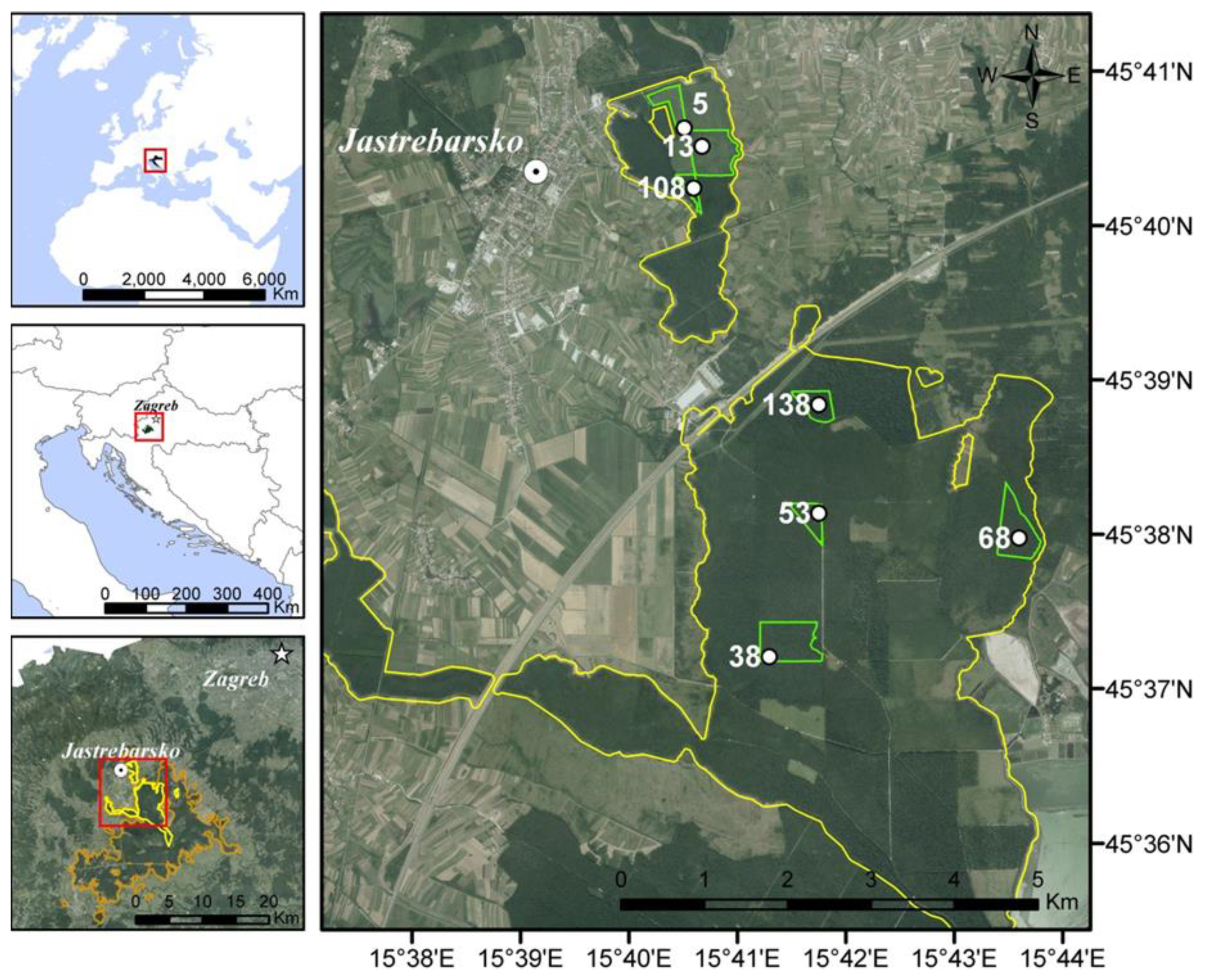
2.1. Study Area and Forest Management Practice

The study area is located in the continental part of Croatia, 35 km southwest from Zagreb, within the managed forests of river Kupa basin (Figure 1). The climate in the area is warm temperate with a mean annual temperature of 10.6 °C and precipitation of 962 mm y−1 for the period 1981–2010 (Appendix A, Figure A1 and Figure A2). Relief is mostly flat with an altitude that ranges from 107 to 130 m a.s.l. Soil texture is loam and clay loam to clay. Soils are hydromorphic, hypogley, eugley, and pseudogley, on clay parent material. Groundwater table level during vegetation period typically varies from −60 to −200 cm [34]. The study site is an even-aged managed forest dominated by Pedunculate Oak (Quercus robur L.), with a significant share of Common hornbeam (Carpinus betulus L.), Black alder (Alnus glutinosa (L.) Geartn.), and Narrow-leaved ash (Fraxinus angustifolia Vahl.) in the tree layer. The understory layer is dominated by hazel (Corylus avellana L.) and common hawthorn (Crataegus monogyna Jacq.) [35].
In Croatia, Pedunculate oak forests cover 225 kha (9% of the total forest area) and they have a growing stock of 66.5 Mm3 (16% of the total growing stock) [36]. They are managed according to the 140 year-long rotations that may be extended if a stand is in a good condition and rotation extension would contribute at attaining uniform distribution of areas with respect to age-classes. Thinnings are conducted every ten years, ending with two or three regeneration cuts in a shelterwood-system during the last 10 years of the rotation. The first cut, termed Stand preparation cut, is aimed at enhancing acorn production of the standing oak trees. In the year of good acorn mast follows the Establishment cut, which aimed at promoting germination of acorns and establishment of young seedlings under the shelter of remaining mother-trees. Finally, 2–3 years after the establishment cut, the Final cut is made and remaining old trees are harvested, which resulted in a regenerated pedunculate oak stand. Furthermore, in the case of poor acorn mast, the acorns from designated seed areas are introduced into the stand before the final cut. On areas of the stand where seedling density remained too low after the final cut, planting of pedunculate oak seedlings of known origin (stand in-filling) must be made within three years after the final cut [37]. Furthermore, a given number of old trees (typically 1 per ha) must be left unharvested for biodiversity. In this way, a natural regeneration under continuous tree crown cover is ensured. After harvest, only coarse wood with a diameter equal to or greater than 7 cm is typically exploited, while all other woody debris and leaf/fruit litter are left at the site. Recently, however, due to demand for wood for energy, the thicker branches are also removed at some sites, while the thinnest one (<2 cm), as well as stumps and litter, are still left in the forest. This approach has been considered sustainable in terms of yield, biodiversity, and ecosystem stability [38], and in Croatia it dates back, more-or-less unchanged, to 1769, when the first forest management plan was made [39]. Regarding present forest management definitions [40], such an approach is classified as close-to-nature forest management.

2.2. Experimental Design and Field Measurements

The experiment was set up at the beginning of 2010. The chronosequence consisted of seven forest stands with different age (5, 13, 38, 53, 68, 108, and 138 years). In each stand, four permanent circular plots with a variable radius (Appendix A, Table A1) were set up within a one-hectare area according to Terrestrial Carbon Observing (TCO) Protocols [41], with the exception of the youngest stand (five years), where five 3 × 3 m plots were set up. Permanent plots represent the base of chronosequence experiment, but they also facilitate other field experiments that are beyond of the scope of this study. In the 38 years old stand, a permanent eddy-covariance system was present [42]. Furthermore, to account for the overall spatial variability of the stand, again with the exception of the youngest stand, additional six to 10 temporary circular plots, with variable radii, were set in a 100 × 100 m grid around each set of permanent plots. The number of additional plots was limited by the size of the corresponding forest compartment (Figure 1). Table 1 gives the main characteristics of each forest stand.

2.2.1. Aboveground Live Biomass Stocks

On each permanent and temporary plot, diameter at breast height (DBH) and tree height were measured for all live trees with DBH > 2 cm. In the youngest stand (five years old), all of the saplings per plot were counted, and on a subsample of 30 saplings per plot, a root collar diameter and a total sapling height were measured. The measurements were taken once a year, at the end of 2010 and 2011.

2.2.2. Dead Wood, Litterfall and Soil

Dead wood includes snags, stumps, and lying dead wood. Snags and stumps diameters and heights were measured, together with live trees. At the centre of each temporary plot, two 10 m crossed intersects were placed and all lying dead wood with a diameter greater than 1 cm was recorded according to the line intersect method [43]. For all dead wood, the decomposition class was estimated according to Hunter (1990) [44]. In the five years old stand, all lying dead wood was piled up after harvesting and deposited on the top of the stumps, therefore the line intersect method could not have been applied, as it assumes a random distribution of lying dead wood. Thus, we measured all stumps, counted all piles within a 50 × 50 m area, and based on the weight of one average pile, estimated that the average biomass of one pile was 20 kg. Dead wood measurements were taken once in 2011.
One litter trap was placed in the centre of each permanent plot and litterfall was collected several times a year both in 2010 and 2011. The samples from litter traps were transported to the laboratory for further processing on the day of collection.
Soil was sampled at four positions within each permanent plot, 5 m away from the plot centre in the directions N, E, S, and W. The forest organic soil layer (forest floor) was sampled with metal collar (d = 16 cm) and separated into two fractions: litter layer (OL) and fragmented and humus layer (OFH), according to the The International Co-operative Programme on Assessment and Monitoring of Air Pollution Effects on Forests (ICP Forests) manual [45]. Mineral soil was sampled with split tube sampler (Eijkelkamp, Giesbeek, The Netherlands) and each soil core was cut into four samples according to a predefined depths (0–5, 5–10, 10–20, and 20–40 cm). The soil was sampled once in 2011. In total, 16 soil core and 16 forest floor samples were taken per stand, representing one age class. Samples of forest organic and mineral soil layers were further processed in the laboratory.

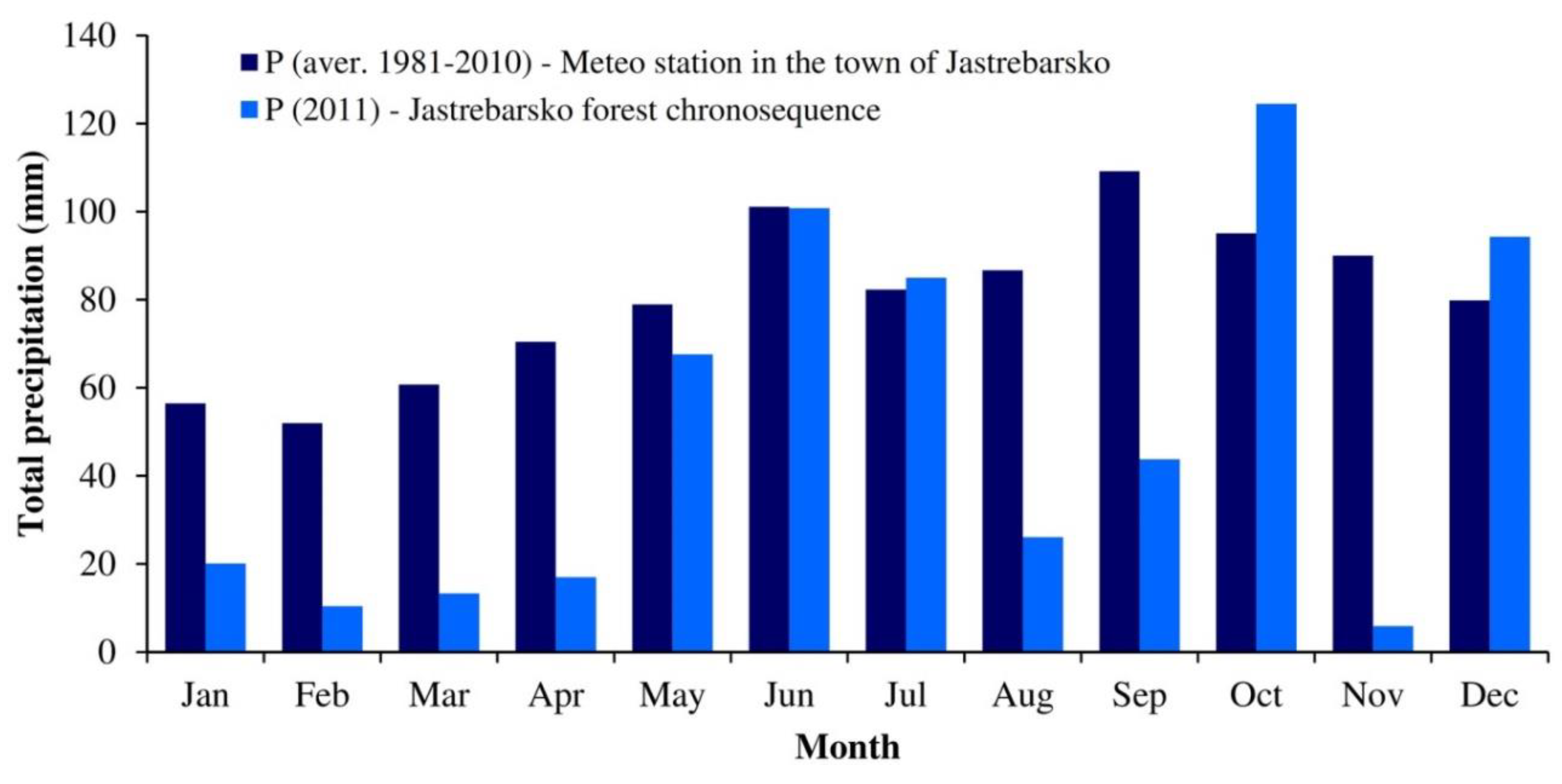
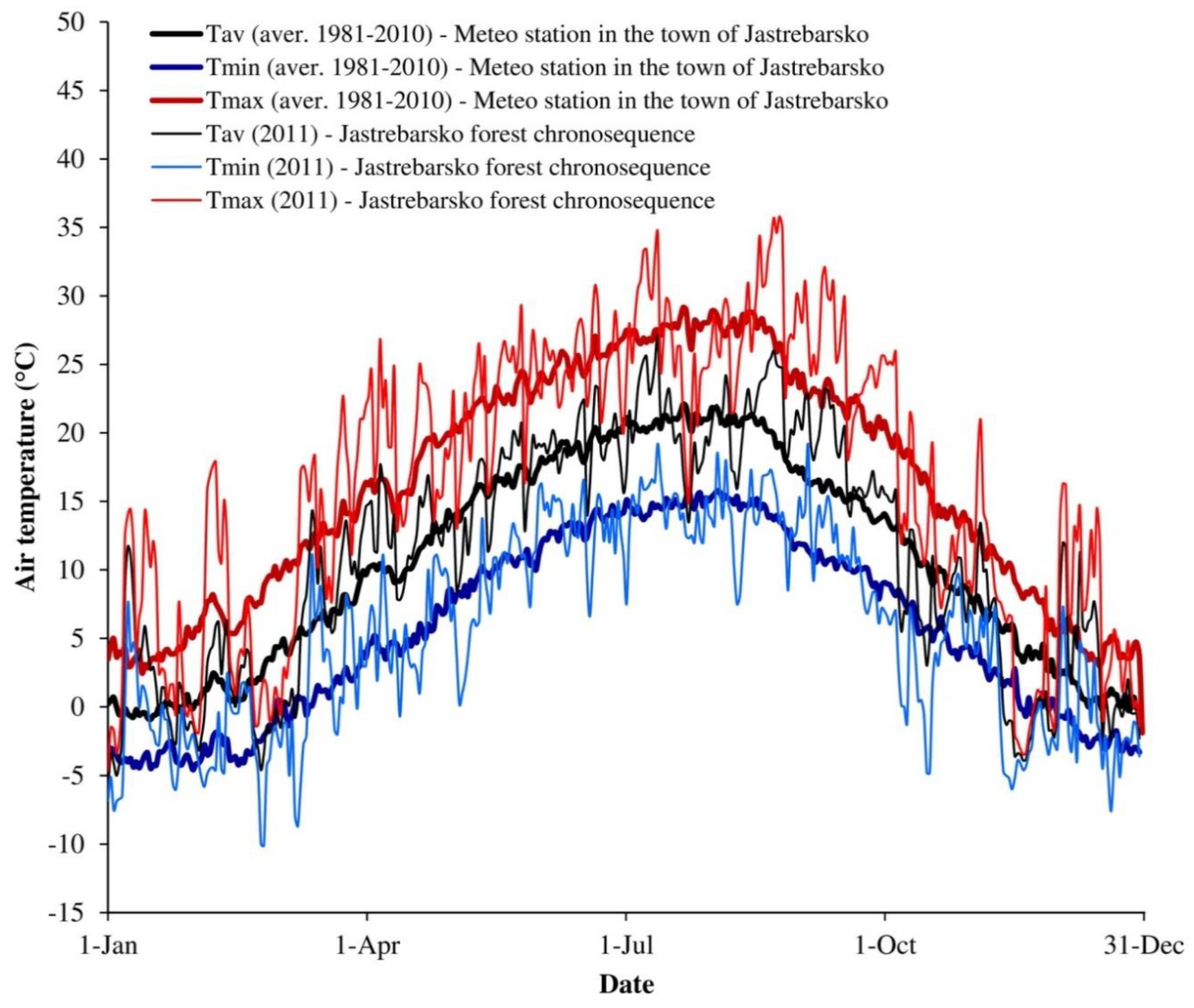
2.2.3. Meteorological Measurements, Soil Respiration and Dead Wood Decomposition Flux

Meteorological and soil respiration measurements were performed in six out of the seven stands (5, 13, 38, 53, 108, and 138 years). A small, custom made, meteorological station was set up inside 2 × 3 m fenced area within each stand. Since December 2010, stations recorded the temperature of air (Tair) and soil (Tsoil) at 5, 10, and 20 cm depths with thermometer sensors DS18B20+ (Maxim Integrated, San Jose, CA, USA) and volumetric soil water content (SWC) at 0–10 cm depth with ECH2O Soil Moisture Sensor 10HS (Decagon Devices, Pullman, WA, USA). At the eddy covariance site (38 years old stand), meteorological conditions were measured by the tower’s weather station [35,42,46]. The period between two successive measurements at all weather stations was 30 min.
Soil CO2 efflux was measured while using an automatic chamber system previously described by Delle Vedove et al. (2007) [47]. In 2011, the soil respiration system (with two to three chambers) was continuously moved among the selected stands every 3–4 days. The measurements were always conducted at the same location within each stand. Inside the previously mentioned fenced area, metal collars, on top of which the flux chamber is fitted, were placed in autumn of 2010 and were left in the ground permanently in order to minimize soil disturbance during 2011 measurement season. When at the location, the system measured the soil CO2 efflux every hour. At eddy covariance site soil respiration system consisted of three to five chambers that were permanently placed into the ground and measurements were performed cyclically, every four hours throughout the year. Data on soil temperature at 5 cm depth (Tsoil5) and soil water content (SWC) were used for soil respiration gap-filling (see chapter 2.5). SWC at field capacity (FC) was estimated to be equal to daily average SWC recorded in spring, before the bud-burst, three days after the SWC started dropping from saturation, similar to FC that was mentioned in the work of Reichstein et al. [48]. The fact that the soil is saturated was observed at the sites (footprints filled-in with water after walking) and corroborated with SWC records (SWC does not increase after the rain events).
In three stands (5, 38, and 108 years), a decomposition experiment was set up with the purpose of estimating decomposition rates for different tree species and dead wood size classes. A detailed description of the decomposition experiment is given in Ostrogović et al. (2015) [49].

2.3. Laboratory Analysis

All the laboratory analyses were performed at the Croatian Forest Research Institute in Jastrebarsko, Croatia. Carbon content in samples from different C pools was measured while using CNS 2000 elemental analyser. Litterfall was separated in leaves and fruits, dried at 105 °C, weighted, and leaves were analysed for C content. The soil was sieved and fine roots (d ≤ 2 mm) separated, washed, dried at 105 °C and weighted. Forest floor samples were pooled to one sample per plot for each fraction (i.e., OL and OFH separately), oven-dried, weighed, and analysed for C content. Mineral soil samples were sieved, oven-dried, weighed, analysed for C content, and soil bulk density was estimated for each soil sample and depth while using a known volume of the sample.

2.4. Carbon Stocks Calculations

Carbon stocks were estimated for live biomass (CLB), dead wood (CDW), forest floor (CFF), and mineral soil layer down to a depth of 40 cm (CM40) and were expressed in Mg C ha−1. CLB was calculated, as described in details below, for aboveground wood, leaf and fruit biomass, belowground fine root biomass, and coarse root biomass while using data on tree diameter and height and applying local allometric equations [50,51,52], basic wood densities [53], biomass equations for twigs and branches [54], measured leaf and fruit biomass, age-dependent coarse root-to-shoot ratios [55,56], measured live fine root biomass, and C content in wood [6], and leaves and fruits [56]. CLB was equal to:
C L B = ( W A G W + W C R + W F R ) · C F W + W L · C F L + W F T · C F F T
where WAGW is aboveground wood biomass, WCR is coarse root biomass, WFR is fine root biomass, WL is leaf biomass, WFT is fruit biomass, CFW is C fraction in wood, CFL is C fraction in leaf, and CFFT is C fraction in fruit.
Aboveground wood biomass was calculated, as follows:
W A G W = V D   >   3 · ρ + W D     3
where VD > 3 is the volume of stems and branches (d > 3 cm on thinner end), ρ is species-specific basic wood density, WD ≤ 3 is biomass of twigs, and branches with d ≤ 3 cm estimated while using a biomass equation factor [54].
Coarse root biomass was calculated, as follows:
W C R = W A G · R S
where WAG is total aboveground biomass (wood, leaf, and fruit), RS is literature age-dependent root-to-shoot ratio [55,56].
CDW was calculated for above and belowground dead wood biomass. Aboveground biomass of snags, stumps, and lying dead wood (i.e., coarse and fine woody debris) was estimated from the volume, while using wood density for different stages of decomposition [6]. The volume of snags and stumps was estimated in the same way as for living trees, and the volume of lying dead wood was estimated while using the transect method [43]. The belowground biomass of snags was calculated in the same way as coarse roots in live biomass. For calculating the belowground biomass of stumps, first the removed aboveground biomass was estimated while using quadratic polynomial function between diameter at 0.3 m (d0.3 m) and aboveground biomass, i.e., W s t u m p = 0.0004 d 0.3   m 2 0.0047 d 0.3   m (p < 0.01, R2 = 0.9829), calibrated on the subsample of 94 trees. Finally, CDW was calculated with the equation:
C D W = ( V D W ρ D E C + V s n a g · ρ D E C   · R S + W s t u m p · R S ) · C F W
where VDW is the total volume of dead wood (snags, stumps, and lying dead wood), ρ D E C is wood density for different stages of decomposition, Vsnag is the volume of snags, and Wstump is the aboveground biomass of stumps, RS is literature age-dependent root-to-shoot ratio [55,56], and CFW is C fraction in wood.
CFF was estimated from the forest floor samples, i.e., OL and OFH fractions, and it was calculated, as follows:
C F F = W O L · C F L + W O F H · C F O F H
where WOL is the dry weight of litter layer, WOFH is the dry weight of fragmented to humified layer, while CFL and CFOFH are carbon fraction in leaves and in fragmented to humified layer, respectively.
CM40 was estimated from mineral soil cores. Each soil core consisted of four samples for different depths, and carbon stock in mineral soil down to 40 cm was calculated while using the following equation:
C M 40 = i = 1 4 ( C F i · ρ B i · h i )
where CFi is carbon fraction in the ith soil layer, ρ B i is the bulk density of the ith soil layer, and hi is the height of the ith soil layer.

2.5. Carbon Fluxes Calculations and Modelling

Main C fluxes estimated in this research were net primary production (NPP), total soil respiration (SR), heterotrophic soil respiration (SRH) from dead coarse roots (SRHCR), and from soil organic matter (SRHSOM) and decomposition (respiration) of dead wood (RDW).
Annual NPP was estimated as the sum of the annual production of wood (NPPW), leaves (NPPL), fruits (NPPFT), and fine roots (NPPFR). NPPW was estimated as the difference between C stocks in wood biomass (aboveground and belowground) between two measurement points in time at each plot, i.e., winter 2010 and 2011. NPPL and NPPFT correspond to annual C stocks in leaves and fruits, respectively, assessed while using litter traps. NPPFR was estimated starting from C stocks in fine roots and assuming that the live fine root fraction on total (live and dead) fine root was 50% [57,58] and that turnover rate for Pedunculate oak fine root was one year−1 [59].
Total NPP was then modelled using gamma function as proposed in Tang et al. (2014) [60].
N P P = k 0 · A G E k 1 · e k 2 · A G E
where k0, k1, and k2 are fitting parameters, and AGE is a stand age.
Starting from measured fluxes, total annual soil respiration at each plot was calculated while using a modified soil respiration model [48,61]:
S R = ( a A G E + b A G E · A G E ) · e ( a R E W + b R E W · R S W C ) · · ( 1 T r e f T 0 1 T s o i l 5 T 0 ) · R S W C R S W C 1 / 2 + R S W C
where AGE is a stand age, RSWC is a relative soil water content (ratio of actual SWC and SWC at field capacity), Tref is a reference temperature (i.e., average temperature for research area in the study period, 11 °C), T0 is the lower temperature limit for the soil respiration (−46 °C), Tsoil5 is soil temperature at 5 cm depth, aAGE, bAGE, aREW, bREW, and RSWC1/2 are model parameters (for more details see Appendix A, Table A2 and Table A3).
Annual SRH was estimated from total soil respiration measurements and from the decomposition of belowground dead wood biomass (i.e., coarse roots of snags and stumps). Following Bond-Lamberty and Thomson (2012) [62] and Subke et al. (2006) [63], we estimated the mean heterotrophic to total soil respiration ratio (SRH:SR) of 0.514 for temperate deciduous managed forests with mean annual precipitation range of 600–1200 mm, mean annual temperature range of 10–15 °C, and with total soil respiration in range of 3–13 t C ha−1 y−1. However, by using solely a constant ratio, we would have not been able to account for the increased share of SRH after management disturbance (i.e., final cut). Therefore, we divided SRH into heterotrophic respiration from coarse roots of stumps and snags (SRHCR) and heterotrophic respiration from other soil organic matter (SRHSOM). We assumed that the decomposition of coarse roots has a decreasing trend during the lifetime of the stand, as proposed in Harmon et al. (2011) [64], while the share of decomposition of soil organic matter in total soil respiration can be considered as constant during the time, as observed by Liu et al. (2015) [65]. SRHCR was estimated as the decomposition of coarse roots biomass of stumps and snags, thus the equation proposed by Olson (1963) [66] was used:
S R H C R = C D W B G ( 1 e k t )
where CDWBG is carbon in belowground dead wood biomass (i.e., coarse roots of stumps and snags), k is decomposition rate of 0.182, i.e., an average for fine woody debris (2 mm–7 cm) of naturally occurring tree species in pedunculate oak forest [49], and t is time of decomposition (i.e., 1 year).
SRHSOM was estimated from remaining total annual soil respiration (i.e., the difference between SR and SRHCR) using a share of heterotrophic to total soil respiration. The following equation was used:
S R H S O M = ( S R S R H C R ) · ( S R H : S R )
where SR is total soil respiration and SRH:SR is heterotrophic to total soil respiration ratio of 0.514 (calculated as described above).
Annual RDW was estimated based on aboveground dead wood biomass and decomposition rates (k) estimated from decomposition experiment [49] and previously published data [67] for fine and coarse woody debris, respectively. The following equation was used:
R D W = W A G D W ( 1 e k t )
where WAGDW is aboveground dead wood biomass, k is decomposition rate, and t is time of decomposition (i.e., 1 year).
Total heterotrophic respiration (RH) was calculated as the sum of SRHCR, SRHSOM, and RDW. The RH was modelled while using a logarithmic function, as follows:
R H = a · ln ( A G E ) + b
where a and b are parameters, and AGE is a stand age. Finally, net ecosystem productivity (NEP) was estimated as the difference between NPP and RH.

2.6. Harvest Carbon Losses and Net Ecosystem Carbon Balance

The estimation of past harvests, particularly for old stands, is challenging not only because data on harvest might be missing (oldest stand is 138 years old, while management records are available only for the last 40 years), but also because the area of given forest compartment might have changed. Therefore, we used measured growing stock data to determine the site yield class of our selected stands in the chronosequence, and we then applied prescribed thinnings for specific site class from local species-specific yield tables [68]. Such an approach carries large uncertainty, but, on the other hand, it reflects the usual management practice. The volume of the final cut was estimated from the amount of C that was assumed to be removed from the oldest stands after the final cut by applying basic wood density for oak and C fraction of wood. Finally, harvest loss (VHL) was obtained as the sum of thinnings and final cut. Cumulative harvest C loss was estimated, as follows:
C H L = A G E 1 A G E 2 V H L ( A G E ) · ρ · C F W
where VHL(AGE) is the prescribed harvested wood volume at a given stand age, ρ is basic wood density for oak, and CFW is the carbon fraction in wood. Typically, dying or standing dead trees are removed during thinnings or final cut. Therefore, C loss from tree mortality can be considered, at least to a great extent, accounted for under harvest C losses.
NECB throughout the rotation was estimated while using two different approaches: the pool-change approach and the component-flux approach. With the pool-change approach, NECB was calculated as the cumulative difference between C stocks in two different stand ages. C stocks in the first year were assumed to be equal to the stocks that remain in the forest after the final cut of the previous stand. For the five years old stand (the youngest stand in our chronosequence), we back-calculated stocks in aboveground live wood biomass, as it would be before the final cut, i.e., at age 0 (so-called “previous stand”), as follows:
C L B A G W = ( V H · ρ · ( 1 + 0.044 ) · C F )
where CLBAGW is aboveground live wood biomass at age 0, VH is harvested volume of five years old stand obtained from previous management plan, ρ is species-specific basic wood density, and 0.044 is an average share of biomass of small branches and twigs (WD ≤ 3) in the total aboveground wood biomass (WAGW) of all trees in 138 years old stand (the oldest stand in our chronosequence).
Applying the relative shares of C stocks, as obtained from 138 years old stand, to CLBAGW at age 0 we estimated C stocks by all forest ecosystem pools. With the final cut, we assumed the following C stocks allocations: all CLB to 0; 4.4% of CLBAGW to CDWAG (representing the biomass of small branches and twigs that were left at the site after harvest); CLBAGW of new stumps (calculated as CDWAG in five years old stand while using an average ρ for all occurring tree species instead of wood density for different stages of decomposition, i.e., 3.9 Mg C ha−1) to CDWAG; CLBFR; and, CLBCR to CDWBG; CLBL; and, CLBFT to CFFOL.
When considering that the final cut did not occur during our experiment, we had to estimate C stocks of a 140 years old stand after the final harvest. To do this, we used data from the 138 years and the 0 years old stands. In short, we estimated the two-year increment of the 138 years old stand, added it to the stock, and then performed a hypothetical final cut and wood removal. Distribution of the remaining carbon stocks by pools in such, 140 years old stand that had been harvested, was modelled based on the shares of carbon in pools of the 0 years old stand. The only difference was that in 140 years CLBAGW of new stumps was estimated as C stocks of a bole with a diameter at the root collar (d0.3 m) calculated from relation DBH = 0.6571 × d0.3 m (p < 0.01, R2 = 0.9953), calibrated on the subsample of 94 trees, with average stump height of 0.24 m (observed at the site) and species-specific basic wood densities.
With the component-flux approach, NECB was calculated as the difference between the cumulative sum of NEP and cumulative harvest C losses.
Finally, NECB from a pool-change approach, i.e., from C stocks (NECB_s), and NECB from component-flux approach, i.e., from C fluxes (NECB_f), were compared.

2.7. Statistical Analysis

Processing of meteorological data and raw data on soil CO2 efflux measurements and modelling of soil respiration, net primary productivity (NPP), and heterotrophic respiration (RH) were performed with STATA 14 software (StataCorp, College Station, TX, USA) [69]. C stocks and fluxes were expressed, unless differently stated, as average values for each stand with standard errors. One-way ANOVA, followed by Tukey post-hoc test, was performed for C stocks and fluxes across the chronosequence.

3. Results

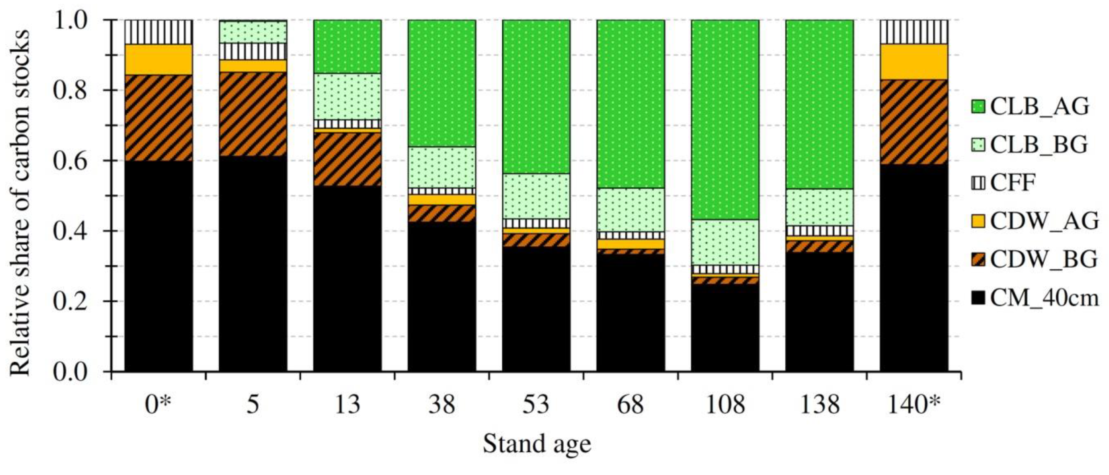
3.1. Carbon Stocks and Their Temporal Evolution

Table 2 reports the C stocks in the different pools. C stocks in live biomass increased with stand age and reached its maximum of 204.9 ± 18.1 Mg C ha−1 at the age of 108 years. The C stocks in dead wood were higher in the younger stands (5, 13, and 38 years) than in the mature stand (108 years). C stocks in forest floor showed a linear increase with stand age (R2 = 0.90, p < 0.004), while C stocks in the top 40 cm of soil mineral layer, although some significant differences were detected among age classes (Table 2), did not show any significant correlation with stand age (R2 = 0.14, p > 0.40). In stands that were older than 50 years, C stocks in forest soil (forest floor and mineral layer) represented 34% of the total.
Most of the C was, on average, stored in live biomass (53%), even though the C distribution among the different pools changed with stand development (Figure 2). In fact, while in the youngest stand (five years), 61% of C was stored in mineral soil layer and the rest of C was mostly stored in dead wood, during stand development, the distribution of C stocks went in favour of live biomass, with the maximum share of 70% reached in the 108 years old stand.

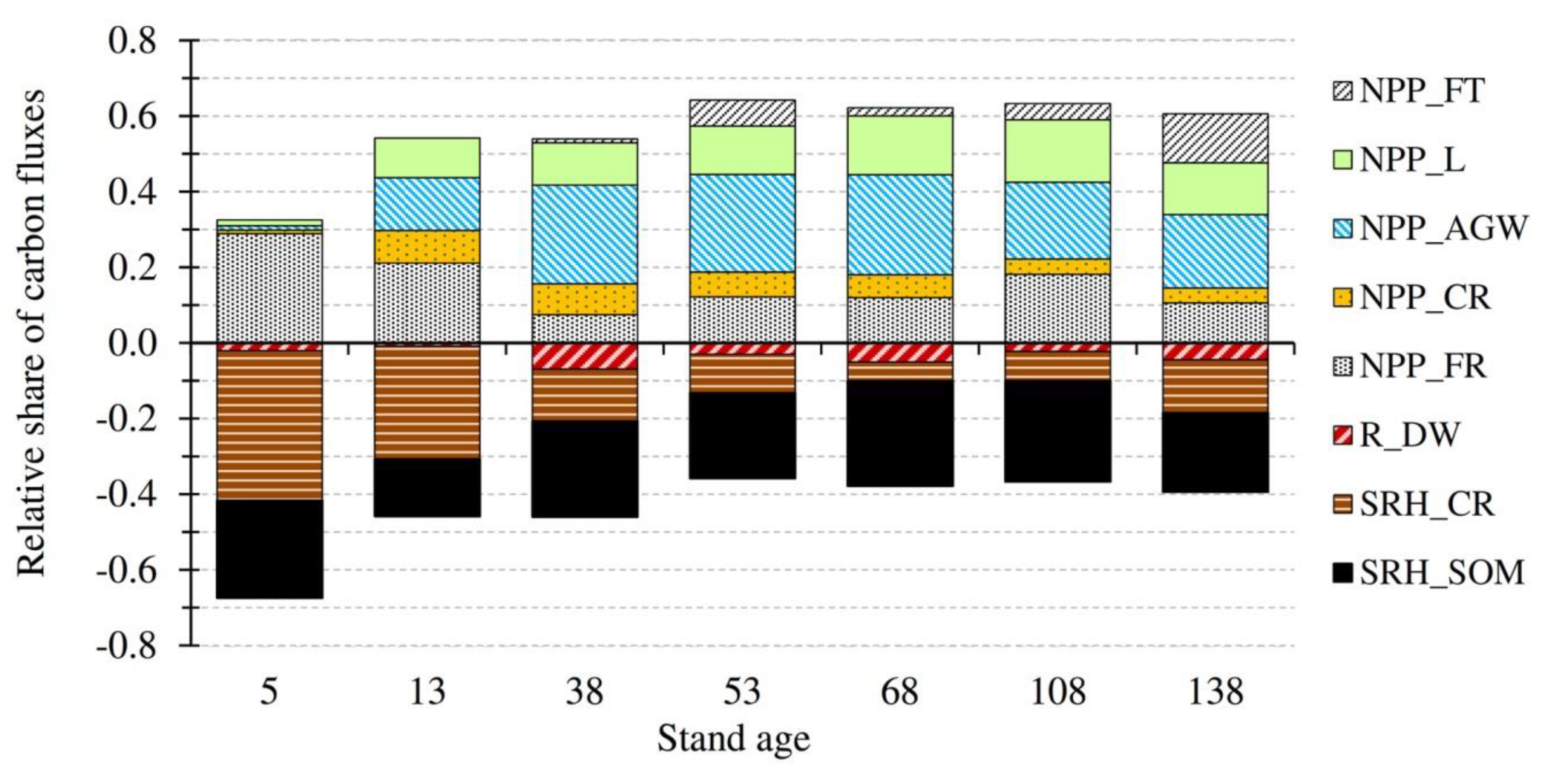
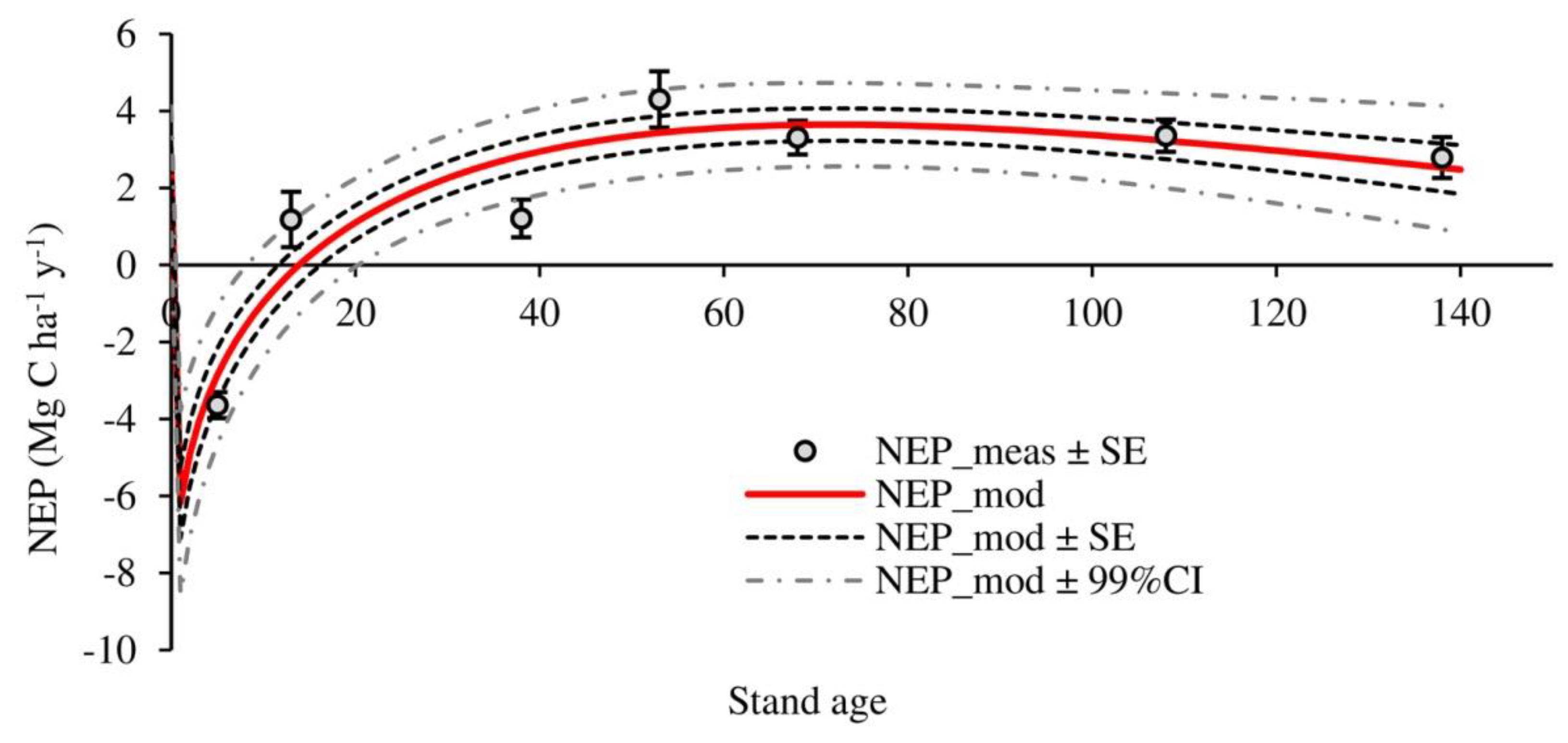
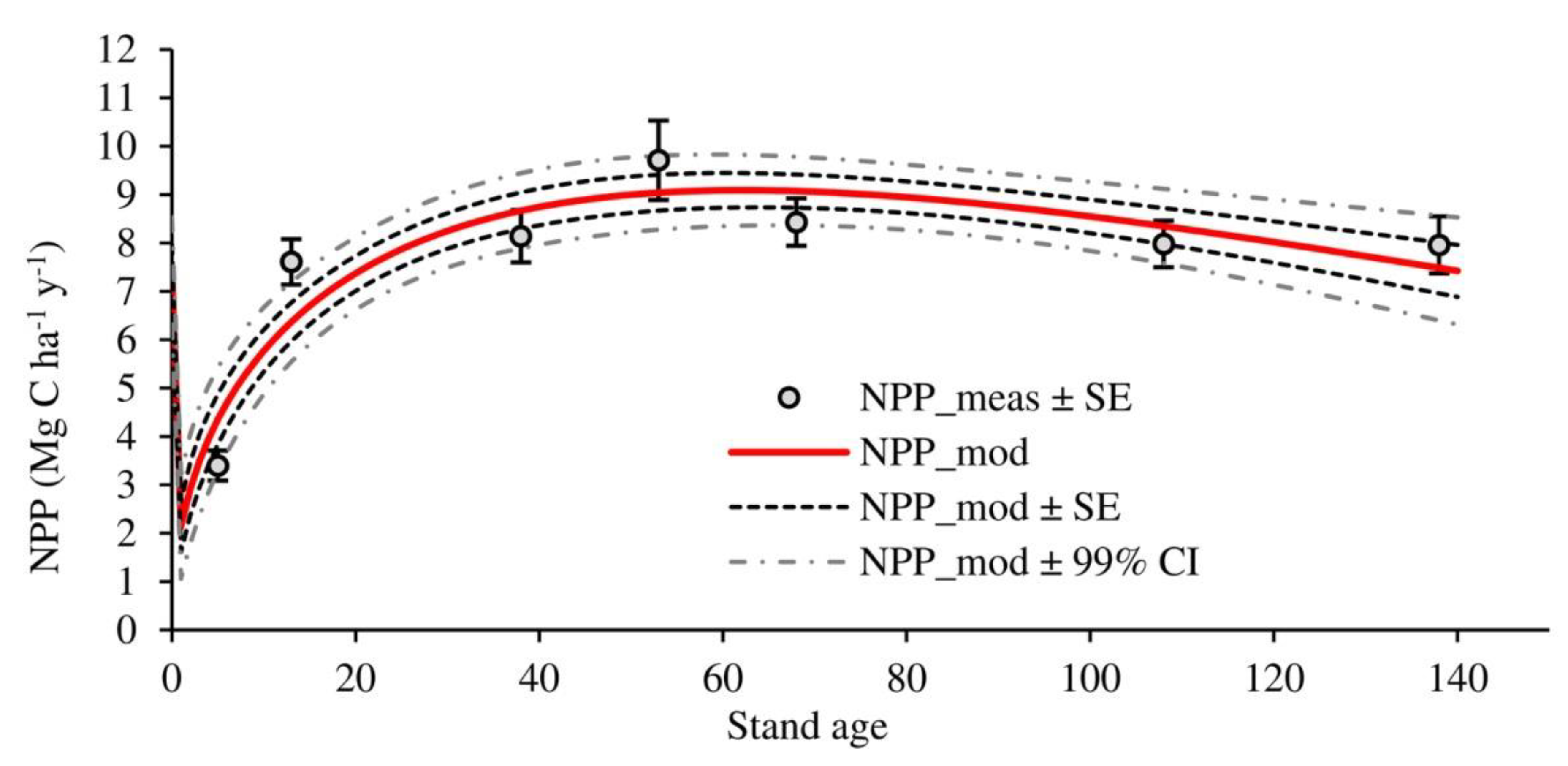
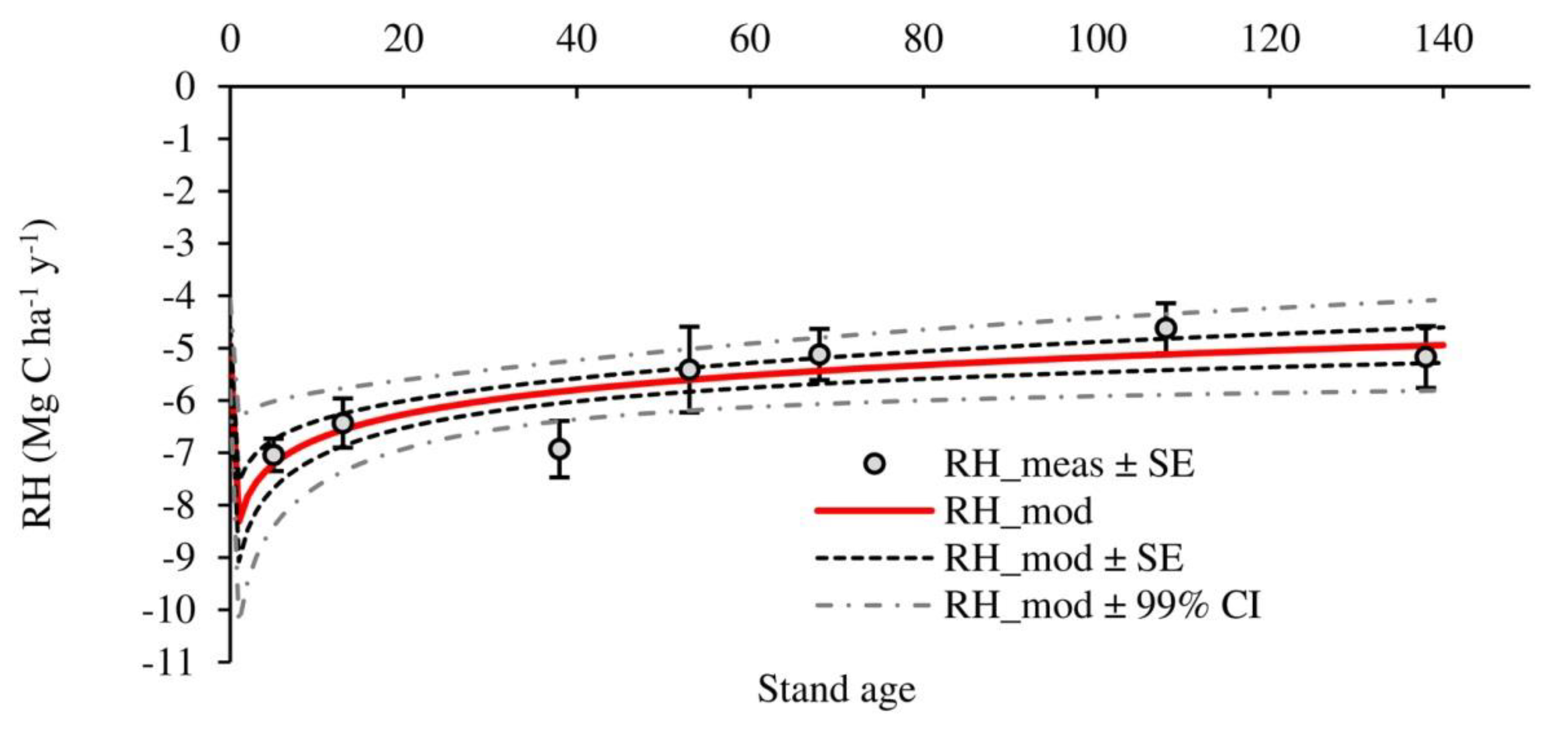
3.2. Temporal Evolution of Carbon Fluxes and Net Ecosystem Productivity

Table 3 reports the main ecosystem C fluxes. Forest ecosystem in-coming carbon fluxes are considered to be positive (NPP), while out-going fluxes are considered as negative (SR and RDW). Mean total NPP along the chronosequence was 7.60 ± 0.75 Mg C ha−1 y−1, with a maximum in the 53 years old stand. A significant difference was only observed for the youngest stand, which showed the lowest value. Leaf biomass production (NPPL) was relatively uniform throughout the chronosequence, with the exception of the youngest stand, where the canopy was not completely closed. Fruit production showed significant differences among the stands, with the highest production in the oldest stand. Fine root production showed high variability, but no age-related trend was observed. SR showed a linear decrease with stand age (R2 = 0.70, p < 0.05), although with low variability (i.e., 11%) among stands. On the contrary, RDW showed significantly higher spatial variability (66%), but no age trend was observed. In the youngest stand, negative fluxes (i.e., SRH and RDW) exceed positive NPP flux, which results with a net carbon loss from the ecosystem (i.e., negative NEP values). By the age of 13 years, NEP became positive and with small fluctuation remained positive throughout the chronosequence. The highest carbon sink was observed in 53 years old stand. Although sink seemingly declined with increasing stand age, the observed NEPs in stands of 53 years and older were not significantly (p < 0.05) different (Table 3).
Share of positive and negative carbon fluxes, as well as the share of below- and aboveground carbon fluxes differed between stands of different age (Figure 3). In the youngest stand, SRHCR accounted for 40% of all fluxes and represented the greatest flux. Second flux in magnitude was fine root productivity that made almost 90% of NPP of the five years old stand. At the age of 13 years, SRH decreased and the share of positive and negative fluxes reached equilibrium at 60:40. By the age of 38 years, the share of above- and belowground NPP fluxes stabilized at 71:29. Share of RDW was on average 3.6% of all fluxes.
The temporal evolution of the main C fluxes was modelled through time (Figure 4). NPP showed age-related trend and was modelled while using eq. 7 (R2 = 0.98, RMSE = 1.2872, n = 28). Table 4 gives the model parameters. Total heterotrophic respiration (RH) also showed an age trend (Figure 5) and was modelled using Equation (10) (R2 = 0.69, RMSE = 0.6259, n = 6). Parameters of the RH model are given in Table 5. Finally, NEP was estimated from NPP and RH and Figure 6 shows its temporal evolution.

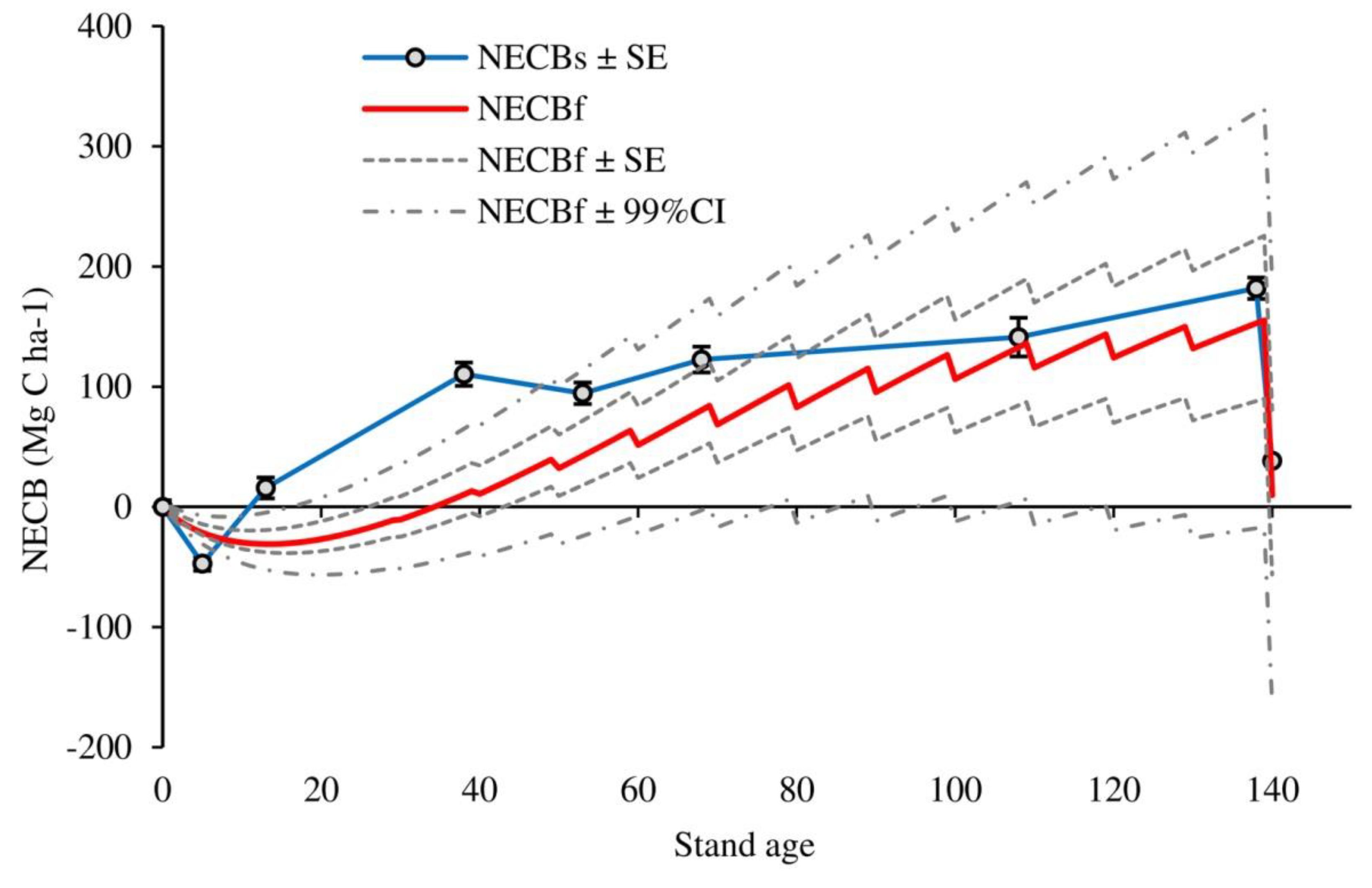
3.3. Harvest Carbon Losses and Net Ecosystem Carbon Balance throughout the Rotation

The cumulative harvest carbon losses (CHL) amounted to 335.18 Mg C ha−1, out of which 187.24 was through thinnings and 147.94 in the final cut. The distribution of CHL among age classes is given in Appendix A (Table A4). NECB calculated from stocks (i.e., pool-change approach) and from fluxes (i.e., component-flux approach) is given in Table 6, while Figure 7 shows its long-term dynamic. The two different approaches showed a clear difference in NECB estimates. Overall, NECB from the pool-change approach (NECBs) was higher than the component-flux approach (NECBf), with a significant difference observed in younger stands (< 50 years). Component-flux gave lower NECB estimates, but with higher uncertainty. NECBs reached greater C loss in the first five years, i.e., −47.1 Mg C ha−1 compared to NECBf C loss of −31 Mg C ha−1 reached at the age of 13 years. According to pool-change approach, the forest became C sink before the age of 13 years, while NECBf remains negative until 35 years. In older stands, the two approaches showed similar NECB values.

4. Discussion

4.1. Carbon Stocks in Different Ecosystem Pools and Their Temporal Evolution

The maximum value of C stocks in live biomass (CLB) observed in our study (204.9 Mg C ha−1) is within the range of published data on deciduous tree species in Europe, e.g., 102 Mg C ha−1 in an oak chronosequence in Austria [11], 172 Mg C ha−1 in a beech chronosequence in Italy [12], 181 Mg C ha−1 in an old-growth mixed forest in UK [13], and 231–233 Mg C ha−1 in an even-aged beech forest in Germany [6]. Understandably, the observed differences in CLB can be linked to differences in stand basal area (BA), where greater BA implies greater CLB and vice versa. Furthermore, stand volume and mean tree height are both very important stand structure elements to be considered in the comparison of this kind. Higher values of CLB observed in Mund (2004) [6] can be attributed to 20% higher stand volume than in our research, while the lower values of CLB in Bruckman et al. (2011) [11] can be explained with lower mean tree height (15–20 %) than in our research. Soil nutrient availability and management differences are other key variables that likely contribute to the observed variability in CLB.
In temperate forest ecosystems, C stocks in dead wood (CDW) are extremely variable [15], and the main controlling factors are stand density, site quality, and forest management frequency and intensity. Average CDW estimated in our research (18 Mg C ha−1) is significantly lower than CDW observed in a managed beech forests in Slovenia (28.4 Mg C ha−1) [70]. Apart from management differences, the stand structure seems to be the likely reason for this. Namely, a significantly higher average number of stumps was observed in beech forest (app. 217 stumps ha−1) compared to our oak chronosequence (average 127 stumps ha−1) [61]. Research dealing with the estimation of CDW sometimes do not account for belowground carbon stocks, i.e., root biomass of stumps and snags [6]. When just aboveground CDW estimated in our research (4.7 Mg C ha−1) are considered, our values are more in line with previous literature data, i.e., 5 Mg C ha−1 in Mund (2004) [6] and 4.2 Mg C ha−1 in Čavlović (2010) [71].
Average C stock in forest floor (CFF) estimated in our study (6 Mg C ha−1) is significantly higher than data published for old black alder (Alnus glutionsa Gaertn.) stand near river Drava in Croatia (2.2 Mg C ha−1) [72], but much lower than value published for 60-year old oak stand in the Netherlands (26.1 Mg C ha−1) [73]. In alder stand, faster decomposition of dead organic matter in forest floor might be attributed to more favourable litter chemical composition (less tannin), higher nitrogen content and higher soil moisture. On the other hand, according to Schulp et al. (2008) [73], forests management activities in the Netherland are less intensive than in many other countries and this might influence CFF accumulation. At our study site, the average thickness of the forest floor was 1.5 cm [61], which is more than 4 times lower than 6.6 cm published in Schulp et al. (2008) [73].
Carbon stocks in mineral soil (CM) depend, among others, on the depth of the soil sampling, which varies among different studies. In this work, we have presented results according to four distinct layers (Table 2) to facilitate comparison with the results from similar works. For example, C stock in the top 15 cm of soil mineral layer (CM_0_15) observed in even-aged beech forests in Germany were 39 and 42 Mg C ha−1 [6] as compared to the average of 45.6 Mg C ha−1 in first 15 cm of soil at our study site. Values for the CM_0_20 (top 20 cm of soil) reported for the beech forest in Italy were disproportionally higher (105 Mg C ha−1) [12] when compared to 58.3 Mg C ha-1 in top 20 cm of soil in our research. A comparison of the average CM_0_20 in our research with the results from other oak forests showed, instead, good agreement. For example, for the sessile oak forest in Austria, Bruckman et al. (2011) [11] reported 38 Mg C ha−1 for CM_0_20, while Hale (2015) [13] for mixed forests in the UK reported 43 and 41 Mg C ha−1 (for old and young growth, respectively). Contrastingly, Schulp et al. (2008) [73] for the CM_0_20 in the 60-year old oak stand in the Netherlands reported 82 Mg C ha−1, which is significantly higher value compared to the averages above, but closer to the value of 59.8 Mg C ha−1 for the 68 years old stand in our chronosequence (Table 2).
The temporal evolution of C stocks distribution by pools was investigated in many studies [5,6,11,12,15,74,75]. The common result in all these studies is that younger stands, up to approx. 30 years of age, have the highest share of C stored in the soil. With time, in managed forests distribution of carbon stocks changes in favour of live biomass, while the C stocks in dead wood biomass show opposite behaviour with the highest values occurring in young stands and then gradually decline. In the case of the pedunculate oak forest (i.e., our chronosequence), most of the C was stored in soil up to approx. 20 years of age. After stand establishment, the share of CLB increases fast, reaching a peak at around 100 years, after when its share starts to decline. CDW has the highest values after the final cut, and then rapidly declines. Such behaviour is the result of management, where most of the dead or dying trees are harvested and extracted during the thinning. A slight increase in the share of CDW that was observed in the oldest stand is mostly the result of an increased number of larger oak stumps remaining after thinning, which can have a very long turnover time.

4.2. Carbon Fluxes and Net Ecosystem Productivity

Net primary productivity (NPP) is one of the main C fluxes in forest ecosystems, and it mostly depends on tree species [76], stand age [10,15,29], and climate [10,15]. The average NPP estimated in our study (7.6 ± 0.75 Mg C ha−1 y−1) is close to the global estimate for temperate deciduous forests published in Luyssaert et al. 2007 (7.38 ± 0.55 Mg C ha−1 y−1) [19] and Pregitzer and Euskirchen 2004 (7 Mg C ha−1 y−1) [15]. The parametrization of the NPP model, as proposed by Tang et al. (2014) [60], which was used in our study, yielded parameter estimates that were highly significant (p < 0.001). Therefore, the parameterized model may be considered reliable for estimating NPP of Pedunculate oak stands growing in similar conditions and managed with a similar management system.
Soil respiration (SR) is the second most important ecosystem C flux. It accounts for the respiration of live roots and microorganisms, and decomposition of forest floor, dead roots, and other soil organic matter. It is influenced by environmental conditions, with high temporal and spatial variability [77]. The temporal dynamic of SR is highly influenced by the dynamic of meteorological conditions, while spatial variability is largely due to soil properties, the activity of microorganism and of the soil fauna, and growth and turnover of fine root biomass [77,78]. In our study, the spatial variability of SR was around 11% across the chronosequence, which is relatively low value when compared to the broad range (10 to 100%) published in Campbell and Law (2005) [78] and Hanson et al. (1993) [79]. The average SR estimated in our research (8.35 ± 0.38 Mg C ha−1 y−1) is similar to soil respiration of oak stand in Belgium, 8.8 ± 0.5 Mg C ha−1 y−1 [80], and SR of oak chronosequence in China, 6.23–8.31 Mg C ha−1 y−1 [81].
Heterotrophic SR (SRH) is recognized as an important component of SR flux [62] with high likelihood for being affected by the climate change, therefore there is a growing interest for the improvement of SRH modelling [82]. Nevertheless, when estimating SRH under uniform environmental conditions, a simple empirical approach, as we used in this research, could provide satisfactory results. SRH estimated in our research (i.e., the sum of SRHCR and SRHSOM) is 5.34 ± 0.38 Mg C ha−1 y−1 and it is close to values that were published in Luan et al. (2011) [81], i.e., 4.31–6.78 Mg C ha−1 y−1. Moreover, the average share of SRH:SR estimated in the present study (65.5%) is within the range 63.2–68.6% published in Liu et al. (2015) [65].
The decomposition of dead wood depends on the debris’ size, soil temperature, and moisture, but also on substrate quality [49,77,83,84]. Substrate quality implies specific chemical composition of the dead wood sample (i.e., share of sugars, proteins, cellulose, lignin, and mineral compounds), which directly depends on tree species and sample size. Higher shares of sugars and proteins in dead wood characterise dead wood of higher substrate quality, which typically exhibits higher rates of decomposition. Decomposition flux also depends on the amount of dead wood C stocks, except for decomposition rates. We were interested in the decomposition flux of aboveground dead wood, as we already included belowground dead wood decomposition in the soil respiration estimates. Decomposition flux RDW in our study ranged from 0.12 to 1.04 Mg C ha−1 y−1, with a mean of 0.48 Mg C ha−1 y−1 across the whole chronosequence. For comparison, the magnitude of RDW corresponds to approx. 11% of SRH. The highest RDW was observed in the 38 years old stand, although the highest C stock in the aboveground dead wood was observed in the oldest stand, where decomposition flux was half of what we estimated in the 38 years old stand. This can be explained with different decomposition rates. According to Ostrogović et al. (2015) [49], one of the main variables explaining the decomposition rates of woody debris is sample size: the smallest samples have the highest decomposition rate, and vice-versa. The higher decomposition flux in the 38 years old stand can be explained with a higher amount of fine woody debris and snags with smaller DBH, than in the other stands (data not shown).
Range of net ecosystem productivity (NEP) in our research spanned from −3.6 to 4.3 Mg C ha−1 y−1, which is close to the values of −2.5 to 5 Mg C ha−1 y−1 that were published for temperate forest ecosystems [7]. In the Pedunculate Oak chronosequence, NEP becomes positive quite early in the development phase, between the stand age of five and 13 years, which is a result of higher NPP fluxes than the total heterotrophic respiration (i.e., the sum of SRH and RDW). Maximum NEP reached at 53 years, which corresponds to the age of highest NPP. At this age, stands still intensively grow in both diameter and height, but also they start with acorn production that accounts, on average, for 10% of total NPP. Later, with age, NEP slowly decreases as the ratio of positive and negative fluxes goes in favour of negative ones. Nevertheless, until the final cut (140 years), Pedunculate oak stands, managed with a close-to-nature management system, retain positive NEP. A similar trend of NEP was observed in Campbell et al. (2004) [7] and De Simon et al. (2012) [12].

4.3. Net Ecosystem Carbon Balance throughout the Rotation Estimated by Different Approaches

The long-term net ecosystem carbon balance (NECB) that was calculated while using the two different approaches showed relevant differences. The pool-change approach yielded in higher NECB estimates with a higher level of precision, although strongly driven with the first and the last data points (Figure 7). Maximum C loss observed for NECBs in the first five years relies on the accuracy of the C stocks estimated for age 0, while the C accumulation observed at the end of the rotation period, before the final cut, is based on C stocks in the oldest chronosequence stand. On the contrary, the component-flux approach showed lower NECB values, but with significantly higher uncertainty, which usually accompanies all modelling and predicting methods [28]. Nevertheless, if chronosequence method is appropriately applied (i.e., if the basic assumptions are met) and if reliable information on forest management activities is available, it might be an indicator that the observed differences between the two C balance estimates, i.e., NECBs and NECBf, could be due to changes in environmental conditions that have occurred over the last century.
Changes in environmental conditions are linked with an increase in both productivity as well as respiration [4,85,86,87]; therefore, their effect on forest C balance is specific to each forest ecosystem. While NECBs is an integrated measure of the long-term C accumulation under both recent (younger stands) and past (older stands) environmental conditions, NECBf revels C accumulation under current meteorology (in this study, 2011). Having that in mind, higher NECBs that were observed in younger stands might be linked with the recent environmental change (i.e., increased temperature, nitrogen deposition, and CO2), favouring an increase in stand productivity rather than in heterotrophic respiration. On the contrary, meteorological conditions in 2011 might have had a stronger effect on respiration (i.e., extremely dry year) [88,89], which results results in lower NEP, and finally NECB. Although NECBf carries high uncertainty, it provides valuable information regarding the possible effects that future droughts could have on long-term forest C balances.

5. Conclusions

When carefully set up, chronosequence is a useful method for estimating the temporal evolution of C stocks and/or carbon fluxes. Nevertheless, when using this method for interpreting the net ecosystem carbon balance over the rotation period, one should be aware of the possible differences in estimates that originate from either the pool-change approach or the component-flux approach. When considering all of the shortcomings of the two approaches, in order to obtain a more reliable estimate of long-term C balance, if possible, a comparison of both approaches is recommended.
Under current close-to-nature forest management, Pedunculate oak forest showed to be sustainable in providing both economic and ecological ecosystem services. While assuming successful regeneration, this forest ecosystem becomes C sink very early in a development phase, between the age of 13 and 35, according to the pool-change and component-flux approach, respectively. During 140 years, this forest provides 604 m3 ha−1 (i.e., 187.2 Mg C ha−1) through thinnings and 477 m3 ha−1 (i.e., 147.9 Mg C ha−1) in the final cut, while preserving, on average, 88.9 Mg C ha−1 in the mineral soil down to 40 cm, 18.2 Mg C ha−1 in dead wood, and 6.0 Mg C ha−1 in the forest floor. Finally, soil C stocks in our chronosequence did not show any age-related trend, which indicated that current management practice has no negative effect on soil carbon stocks.

Author Contributions

M.Z.O.S. and H.M. wrote the paper with equal contributions, prepared all data and made all tables and figures; M.Z.O.S., H.M. and G.A. conceptualized the experiment; G.D.V. designed and G.D.V. and G.A. constructed an automated chamber system; All Authors contributed to the interpretation of the results and to the discussion.

Funding

This research was funded by projects: Carbon balance and carbon cycling in young Pedunculate oak (Quercus robur L.) stands, funded by the Croatian Forest Ltd. (OKFŠ 2009–2010); Sustainability of carbon storage in managed forest of pedunculate oak, funded by the Croatian Forest Ltd. (OKFŠ 2011–2013); Estimating and forecasting forest ecosystems productivity by integrating field measurements, remote sensing and modelling—EFFEctivity, funded by the Croatian Science Foundation (HRZZ-UIP-11-2013-2492).

Acknowledgments

We would like to express our gratitude to the technicians of the Croatian Forest Research Institute who helped in setting-up, maintenance and measurements of sampling plots. Special thanks go to Alessandro Peressotti and Diego Chiabà for their help in setting up the soil respiration systems. We are grateful to three anonymous Reviewers and to the Academic Editor for their valuable comments that helped improve the manuscript.

Conflicts of Interest

The authors declare no conflict of interest. The founding sponsors had no role in the design of the study; in the collection, analyses, or interpretation of data; in the writing of the manuscript, and in the decision to publish the results.

Appendix A

Figure A1. Minimum, maximum and mean daily air temperature at the meteorological station in the town of Jastrebarsko (1981–2010 average; thick lines) and at the 38 years old stand in Jastrebarsko forest during the year 2011 (thin lines).
Forests 10 00814 g0a1
Figure A2. Monthly precipitation at the meteorological station in the town of Jastrebarsko (1981–2010 average; dark blue bars) and at the 38 years old stand in Jastrebarsko forest during 2011 (pale blue bars).
Forests 10 00814 g0a2
Table A1. Plot radius (m), dependent on the stand age and diameter at breast height of the sampled tree.
DBH (cm)Age Class *
I. (1–20 y)II. (21–40 y)III. (41–60 y)IV. (61–80 y)VI. (101–120)VII. (121–140)
2–5222222
6–103.53.53.53.53.53.5
11–307810121617
31–507813131617
51–807813131617
>8056.4 (1 ha)56.456.456.456.456.4
* There was no stand in the V. age class (80–100 y) within the Jastrebarsko forest that would meet the criteria required to be included in the chronosequence. (Note on the reading the table: e.g., for the III age class, all trees with DBH of 2–5 cm were measured within 2 m radius from the plot centre, and within 3.5 m radius all trees with DBH 6–10 cm, and within 10 m radius all trees with DBH of 11–30 cm were measured, etc.).
Table A2. Parameter estimates of soil respiration model (Equation (8)) parameterized for stands older than 5 years (i.e., without complete crown cover).
ParameterValueStandard Errort Valuep ValueLower Conf. LimitUpper Conf. Limit
R = 0.9069; R2 = 0.8225; n = 1313
aAGE2.76520.092229.98<0.00012.58432.9461
bAGE−0.00470.0004−11.16<0.0001−0.0055−0.0039
aREW157.000521.38137.34<0.0001115.0550198.9459
bREW376.035630.003712.53<0.0001317.1749434.8963
RSWC1/20.09850.02274.34<0.00010.05400.1430
Table A3. Parameter estimates of soil respiration model * parameterized for youngest 5 years old stand (i.e., without complete crown cover).
ParameterValueStandard Errort Valuep ValueLower Conf. LimitUpper Conf. Limit
R = 0.9096; R2 = 0.8274; n = 192
Rref4.82740.78136.18<0.00013.28636.3685
E0507.843725.156620.19<0.0001458.2199557.4675
RSWC1/21.03420.28863.580.00040.46501.6035
*SR model used for the 5-year-old stand is S R = R ref × e E 0 × ( 1 T ref T 0 1 T S 5 T 0 ) × RSWC RSWC 1 / 2 + RSWC .
Table A4. Cumulative harvest carbon losses throughout the rotation.
Age ClassHarvest
(m3 ha−1)
Cum. Harvest
(m3 ha−1)
Harvest C Loss
(Mg C ha−1)
Cum. Harvest C Loss
(Mg C ha−1)
Source
20000.000.00Local species-specific yield tables (Špiranec 1975)
Pedunculate Oak
II site class
30551.551.55
4017225.276.82
50345610.5417.36
605010615.5032.86
706216819.2252.08
807123922.0174.09
907531423.2597.34
1007639023.56120.90
1107546523.25144.15
1207253722.32166.47
1306760420.77187.24
1404771081147.94335.18Estimated *
* Based on the yield tables (thinnings) and the volume in the oldest, 138 years old, stand in the chronosequence (final harvest).

References

  1. Pan, Y.D.; Birdsey, R.A.; Fang, J.Y.; Houghton, R.; Kauppi, P.E.; Kurz, W.A.; Phillips, O.L.; Shvidenko, A.; Lewis, S.L.; Canadell, J.G.; et al. A Large and Persistent Carbon Sink in the World’s Forests. Science 2011, 333, 988–993. [Google Scholar] [CrossRef] [PubMed]
  2. FAO. State of the World’s Forests; Food and Agriculture Organization of the United Nations: Rome, Italy, 2009. [Google Scholar]
  3. Fisher, B.; Turner, R.K. Ecosystem services: Classification for valuation. Biol. Conserv. 2008, 141, 1167–1169. [Google Scholar] [CrossRef]
  4. Ciais, P.; Schelhaas, M.J.; Zaehle, S.; Piao, S.L.; Cescatti, A.; Liski, J.; Luyssaert, S.; Le-Maire, G.; Schulze, E.D.; Bouriaud, O.; et al. Carbon accumulation in European forests. Nat. Geosci. 2008, 1, 425–429. [Google Scholar] [CrossRef]
  5. Law, B.E.; Sun, O.J.; Campbell, J.; Van Tuyl, S.; Thornton, P.E. Changes in carbon storage and fluxes in a chronosequence of ponderosa pine. Glob. Chang. Biol. 2003, 9, 510–524. [Google Scholar] [CrossRef]
  6. Mund, M. Carbon Pools of European Beech Forests (Fagus sylvatica) Under Different Silvicultural Management. Doctoral Dissertation, University of Göttingen, Göttingen, Germany, 2004. [Google Scholar]
  7. Campbell, J.L.; Sun, O.J.; Law, B.E. Disturbance and net ecosystem production across three climatically distinct forest landscapes. Glob. Biogeochem. Cycles 2004, 18. [Google Scholar] [CrossRef] [Green Version]
  8. Hedde, M.; Aubert, M.; Decaens, T.; Bureau, F. Dynamics of soil carbon in a beechwood chronosequence forest. For. Ecol. Manag. 2008, 255, 193–202. [Google Scholar] [CrossRef]
  9. Marjanović, H.; Alberti, G.; Balogh, J.; Czóbel, S.; Horváth, L.; Jagodics, A.; Nagy, Z.; Ostrogović, M.Z.; Peressotti, A.; Führer, E. Measurements and estimations of biosphere-atmosphere exchange of greenhouse gases—Forests. In Atmospheric Greenhouse Gases: The Hungarian Perspective; Haszpra, L., Ed.; Springer: New York, NY, USA, 2010; pp. 121–156. [Google Scholar]
  10. Tupek, B.; Zanchi, G.; Verkerk, P.J.; Churkina, G.; Viovy, N.; Hughes, J.K.; Lindner, M. A comparison of alternative modelling approaches to evaluate the European forest carbon fluxes. For. Ecol. Manag. 2010, 260, 241–251. [Google Scholar] [CrossRef]
  11. Bruckman, V.J.; Yan, S.; Hochbichler, E.; Glatzel, G. Carbon pools and temporal dynamics along a rotation period in Quercus dominated high forest and coppice with standards stands. For. Ecol. Manag. 2011, 262, 1853–1862. [Google Scholar] [CrossRef]
  12. De Simon, G.; Alberti, G.; Delle Vedove, G.; Zerbi, G.; Peressotti, A. Carbon stocks and net ecosystem production changes with time in two Italian forest chronosequences. Eur. J. For. Res. 2012, 131, 1297–1311. [Google Scholar] [CrossRef]
  13. Hale, K. Long-Term Carbon Storage in a Semi-Natural British Woodland. Doctoral Dissertation, University of Liverpool, Liverpool, UK, 2015. [Google Scholar]
  14. Lundmark, T.; Bergh, J.; Nordin, A.; Fahlvik, N.; Poudel, B.C. Comparison of carbon balances between continuous-cover and clear-cut forestry in Sweden. Ambio 2016, 45, S203–S213. [Google Scholar] [CrossRef]
  15. Pregitzer, K.S.; Euskirchen, E.S. Carbon cycling and storage in world forests: Biome patterns related to forest age. Glob. Chang. Biol 2004, 10, 2052–2077. [Google Scholar] [CrossRef]
  16. Hlasny, T.; Barcza, Z.; Fabrika, M.; Balazs, B.; Churkina, G.; Pajtik, J.; Sedmak, R.; Turcani, M. Climate change impacts on growth and carbon balance of forests in Central Europe. Clim. Res. 2011, 47, 219–236. [Google Scholar] [CrossRef]
  17. Vicca, S.; Luyssaert, S.; Penuelas, J.; Campioli, M.; Chapin, F.S.; Ciais, P.; Heinemeyer, A.; Hogberg, P.; Kutsch, W.L.; Law, B.E.; et al. Fertile forests produce biomass more efficiently. Ecol. Lett. 2012, 15, 520–526. [Google Scholar] [CrossRef] [PubMed]
  18. Alberti, G.; Vicca, S.; Inglima, I.; Belelli-Marchesini, L.; Genesio, L.; Miglietta, F.; Marjanović, H.; Martinez, C.; Matteucci, G.; D’Andrea, E.; et al. Soil C: N stoichiometry controls carbon sink partitioning between above-ground tree biomass and soil organic matter in high fertility forests. Iforest 2015, 8, 195–206. [Google Scholar] [CrossRef]
  19. Luyssaert, S.; Inglima, I.; Jung, M.; Richardson, A.D.; Reichstein, M.; Papale, D.; Piao, S.L.; Schulzes, E.D.; Wingate, L.; Matteucci, G.; et al. CO2 balance of boreal, temperate, and tropical forests derived from a global database. Glob. Chang. Biol. 2007, 13, 2509–2537. [Google Scholar] [CrossRef]
  20. Campioli, M.; Vicca, S.; Luyssaert, S.; Bilcke, J.; Ceschia, E.; Chapin, F.S.; Ciais, P.; Fernandez-Martinez, M.; Malhi, Y.; Obersteiner, M.; et al. Biomass production effciency controlled by management in temperate and boreal ecosystems. Nat. Geosci. 2015, 8, 843–846. [Google Scholar] [CrossRef]
  21. Verlinden, M.S.; Broeckx, L.S.; Zona, D.; Berhongaray, G.; De Groote, T.; Serrano, M.C.; Janssens, I.A.; Ceulemans, R. Net ecosystem production and carbon balance of an SRC poplar plantation during its first rotation. Biomass Bioenerg. 2013, 56, 412–422. [Google Scholar] [CrossRef] [Green Version]
  22. Price, D.T.; Halliwell, D.H.; Apps, M.J.; Kurz, W.A.; Curry, S.R. Comprehensive assessment of carbon stocks and fluxes in a Boreal-Cordilleran forest management unit. Can. J. For. Res. 1997, 27, 2005–2016. [Google Scholar] [CrossRef]
  23. Scott, N.A.; Rodrigues, C.A.; Hughes, H.; Lee, J.T.; Davidson, E.A.; Dail, D.B.; Malerba, P. Changes in carbon storage and net carbon exchange one year after an initial shelterwood harvest at Howland Forest, ME. Environ. Manag. 2004, 33, S9–S22. [Google Scholar] [CrossRef]
  24. Chapin, F.S.; Woodwell, G.M.; Randerson, J.T.; Rastetter, E.B.; Lovett, G.M.; Baldocchi, D.D.; Clark, D.A.; Harmon, M.E.; Schimel, D.S.; Valentini, R.; et al. Reconciling carbon-cycle concepts, terminology, and methods. Ecosystems 2006, 9, 1041–1050. [Google Scholar] [CrossRef]
  25. Schulze, E.D. Biological control of the terrestrial carbon sink. Biogeosciences 2006, 3, 147–166. [Google Scholar] [CrossRef] [Green Version]
  26. Teets, A.; Fraver, S.; Hollinger, D.Y.; Weiskittel, A.R.; Seymour, R.S.; Richardson, A.D. Linking annual tree growth with eddy-flux measures of net ecosystem productivity across twenty years of observation in a mixed conifer forest. Agric. For. Meteorol. 2018, 249, 479–487. [Google Scholar] [CrossRef]
  27. Pretzsch, H.; Biber, P.; Schutze, G.; Uhl, E.; Rotzer, T. Forest stand growth dynamics in Central Europe have accelerated since 1870. Nat. Commun 2014, 5. [Google Scholar] [CrossRef] [PubMed]
  28. Lindner, M.; Maroschek, M.; Netherer, S.; Kremer, A.; Barbati, A.; Garcia-Gonzalo, J.; Seidl, R.; Delzon, S.; Corona, P.; Kolstrom, M.; et al. Climate change impacts, adaptive capacity, and vulnerability of European forest ecosystems. For. Ecol. Manag. 2010, 259, 698–709. [Google Scholar] [CrossRef]
  29. Mund, M.; Kummetz, E.; Hein, M.; Bauer, G.A.; Schulze, E.D. Growth and carbon stocks of a spruce forest chronosequence in central Europe. For. Ecol. Manag. 2002, 171, 275–296. [Google Scholar] [CrossRef]
  30. Johnson, E.A.; Miyanishi, K. Testing the assumptions of chronosequences in succession. Ecol. Lett. 2008, 11, 419–431. [Google Scholar] [CrossRef]
  31. Walker, L.R.; Wardle, D.A.; Bardgett, R.D.; Clarkson, B.D. The use of chronosequences in studies of ecological succession and soil development. J. Ecol. 2010, 98, 725–736. [Google Scholar] [CrossRef]
  32. Löf, M.; Brunet, J.; Filyushkina, A.; Lindbladh, M.; Skovsgaard, J.P.; Felton, A. Management of oak forests: Striking a balance between timber production, biodiversity and cultural services. Int. J. Biodivers. Sci. Ecosyst. Serv. Manag. 2016, 12, 59–73. [Google Scholar] [CrossRef]
  33. Haavik, L.J.; Billings, S.A.; Guldin, J.M.; Stephen, F.M. Emergent insects, pathogens and drought shape changing patterns in oak decline in North America and Europe. For. Ecol. Manag. 2015, 354, 190–205. [Google Scholar] [CrossRef]
  34. Mayer, B. Hidropedološki odnosi na području nizinskih šuma Pokupskog bazena. Radovi Šumar. Inst. Jastrebar. 1996, 31, 37–89. (In Croatian) [Google Scholar]
  35. Marjanović, H.; Ostrogović, M.Z.; Alberti, G.; Balenović, I.; Paladinić, E.; Indir, K.; Peressotti, A.; Vuletić, D. Carbon Dynamics in Younger Stands of Pedunculate Oak during Two Vegetation Periods. Sumar. List 2011, 135, 59–73. [Google Scholar]
  36. Croatian Forests Ltd. Forest Management Area Plan for the Republic of Croatia for the Period 2016–2025; Croatian Forests Ltd: Zagreb, Croatia, 2016. Available online: https://poljoprivreda.gov.hr/istaknute-teme/sume-112/sumarstvo/sumskogospodarska-osnova-2016-2025/250 (accessed on 17 July 2019). (In Croatian)
  37. Ordinance on Forest Management; Official Gazette 97; Narodne novine: Zagreb, Croatia, 2018; Available online: https://narodne-novine.nn.hr/clanci/sluzbeni/2018_11_97_1875.html (accessed on 17 July 2019).
  38. Klepac, D.; Fabijanić, G. Management of Pedunculate oak forest. In Monography: Pedunculate Oak in Croatia; Klepac, D., Ed.; Croatian Academy of Science and Art and Croatian Forests Ltd.: Zagreb, Croatia, 1996; pp. 257–272. (In Croatian) [Google Scholar]
  39. Meštrović, Š. Pravilnik o izradi šumskoprivrednih osnova, osnova gospodarenja i programa za unapređenja šuma u svjetlu šumarske znanosti. Šumar. List. 1978, 102, 352–364. (In Croatian) [Google Scholar]
  40. Duncker, P.S.; Barreiro, S.M.; Hengeveld, G.M.; Lind, T.; Mason, W.L.; Ambrozy, S.; Spiecker, H. Classification of Forest Management Approaches: A New Conceptual Framework and Its Applicability to European Forestry. Ecol. Soc. 2012, 17. [Google Scholar] [CrossRef]
  41. Law, B.E.; Arkebauer, T.; Campbell, J.L.; Chen, J.; Sun, O.; Schwartz, M.; van Ingen, C.; Verma, S. Terrestrial Carbon Observing Protocols for Vegetation Sampling and Data Submission; Food and Agriculture Organization of the United Nations: Rome, Italy, 2008. [Google Scholar]
  42. Anić, M.; Sever, M.Z.O.; Alberti, G.; Balenović, I.; Paladinić, E.; Peressotti, A.; Tijan, G.; Večenaj, Z.; Vuletić, D.; Marjanović, H. Eddy Covariance vs. Biometric Based Estimates of Net Primary Productivity of Pedunculate Oak (Quercus robur L.) Forest in Croatia during Ten Years. Forests 2018, 9. [Google Scholar] [CrossRef]
  43. Van Wagner, C.E. The Line Intersect Method in Forest Fuel Sampling. For. Sci. 1968, 14, 20–26. [Google Scholar]
  44. Hunter, M.L. Wildlife, Forest, and Forestry: Principles of Managing Forests for Biological Diversity; Prentice-Hall: Englewood Cliffs, NJ, USA, 1990. [Google Scholar]
  45. Cools, N.; De Vos, B. Part X: Sampling and Analysis of Soil. In Manual on Methods and Criteria for Harmonized Sampling, Assessment, Monitoring and Analysis of the Effects of Air Pollution on Forests, 1st ed.; UNECE ICP Forests Programme Co-Ordinating Centre, Ed.; Thünen Institute of Forest Ecosystems: Eberswalde, Germany, 2016; p. 115. [Google Scholar]
  46. Matić, S.; Anić, I. One year since the establishment of a research station for intensive monitoring of carbon cycling in a Pedunculate oak stand—What have we learned? In Proceedings of the Scientific Symposium Forests of Pedunculate Oak in Changed Site and Management Conditions; Croatian Academy of Science and Art: Zagreb, Croatia, 2008; pp. 193–207. [Google Scholar]
  47. Delle Vedove, G.; Alberti, G.; Peressotti, A.; Inglima, I.; Zuliani, M.; Zerbi, G. Automated monitoring of soil respiration: An improved automatic chamber system. Italian J Agron. 2007, 2, 377–382. [Google Scholar] [CrossRef]
  48. Reichstein, M.; Rey, A.; Freibauer, A.; Tenhunen, J.; Valentini, R.; Banza, J.; Casals, P.; Cheng, Y.F.; Grunzweig, J.M.; Irvine, J.; et al. Modeling temporal and large-scale spatial variability of soil respiration from soil water availability, temperature and vegetation productivity indices. Glob. Biogeochem. Cycle 2003, 17. [Google Scholar] [CrossRef]
  49. Ostrogović, M.Z.; Marjanović, H.; Balenović, I.; Sever, K.; Jazbec, A. Decomposition of fine woody debris from main tree species in lowland oak forests. Pol. J. Ecol. 2015, 63, 247–259. [Google Scholar] [CrossRef]
  50. Špiranec, M. Allometric equations. Rad Šumar. Inst. Jastrebar. 1975, 22, 1–262. (In Croatian) [Google Scholar]
  51. Cestar, D.; Kovačić, D.J. Wood volume tables for Black Alder and Black Locust. Rad Šumar. Inst. Jastrebar. 1982, 49, 1–149, (In Croatian with English Summary). [Google Scholar]
  52. Cestar, D.; Kovačić, D.J. Wood volume tables for Narrow-leaved Ash (Fraxinus parvifolia Auct.). Rad Šumar. Inst. Jastrebar. 1984, 60, 1–178, (In Croatian with English Summary). [Google Scholar]
  53. Ugrenović, A. Forestry Encyclopaedia I; Miroslav Krleža Institute of Lexicography: Zagreb, Croatia, 1959. (In Croatian) [Google Scholar]
  54. Balboa-Murias, M.A.; Rojo, A.; Alvarez, J.G.; Merino, A. Carbon and nutrient stocks in mature Quercus robur L. stands in NW Spain. Ann. For. Sci. 2006, 63, 557–565. [Google Scholar] [CrossRef]
  55. Cairns, M.A.; Brown, S.; Helmer, E.H.; Baumgardner, G.A. Root biomass allocation in the world’s upland forests. Oecologia 1997, 111, 1–11. [Google Scholar] [CrossRef] [PubMed]
  56. Genet, H.; Breda, N.; Dufrene, E. Age-related variation in carbon allocation at tree and stand scales in beech (Fagus sylvatica L.) and sessile oak (Quercus petraea (Matt.) Liebl.) using a chronosequence approach. Tree Physiol. 2010, 30, 177–192. [Google Scholar] [CrossRef] [PubMed]
  57. Joslin, J.D.; Gaudinski, J.B.; Torn, M.S.; Riley, W.J.; Hanson, P.J. Fine-root turnover patterns and their relationship to root diameter and soil depth in a C-14-labeled hardwood forest. New Phytol. 2006, 172, 523–535. [Google Scholar] [CrossRef] [PubMed]
  58. Jackson, R.B.; Mooney, H.A.; Schulze, E.D. A global budget for fine root biomass, surface area, and nutrient contents. Proc. Natl. Acad. Sci. USA 1997, 94, 7362–7366. [Google Scholar] [CrossRef] [PubMed] [Green Version]
  59. Pietsch, S.A.; Hasenauer, H.; Thornton, P.E. BGC-model parameters for tree species growing in central European forests. For. Ecol. Manag. 2005, 211, 264–295. [Google Scholar] [CrossRef]
  60. Tang, J.W.; Luyssaert, S.; Richardson, A.D.; Kutsch, W.; Janssens, I.A. Steeper declines in forest photosynthesis than respiration explain age-driven decreases in forest growth. Proc. Natl. Acad. Sci. USA 2014, 111, 8856–8860. [Google Scholar] [CrossRef] [Green Version]
  61. Ostrogović, M.Z. Carbon Stocks and Carbon Balance of an Even Aged Pedunculate Oak (Quercus robur L.) Forest in Kupa River Basin. Doctoral Dissertation, Faculty of Forestry, University of Zagreb, Zagreb, Croatia, 2013. [Google Scholar]
  62. Bond-Lamberty, B.P.; Thomson, A.M. A Global Database of Soil Respiration Data; Version 2.0; Oak Ridge National Laboratory Distributed Active Archive Center: Oak Ridge, TN, USA. Available online: http://daac.ornl.gov (accessed on 12 March 2018).
  63. Subke, J.A.; Inglima, I.; Cotrufo, M.F. Trends and methodological impacts in soil CO2 efflux partitioning: A meta-analytical review. Glob. Chang. Biol. 2006, 12, 1813. [Google Scholar] [CrossRef]
  64. Harmon, M.E.; Bond-Lamberty, B.; Tang, J.W.; Vargas, R. Heterotrophic respiration in disturbed forests: A review with examples from North America. J. Geophys. Res. Biogeosci. 2011, 116. [Google Scholar] [CrossRef]
  65. Liu, Q.; Zhao, C.Z.; Cheng, X.Y.; Yin, H.J. Soil respiration and carbon pools across a range of spruce stand ages, Eastern Tibetan Plateau. Soil Sci. Plant. Nutr. 2015, 61, 440–449. [Google Scholar] [CrossRef]
  66. Olson, J.S. Energy-Storage and Balance of Producers and Decomposers in Ecological-Systems. Ecology 1963, 44, 322–331. [Google Scholar] [CrossRef]
  67. Mattson, K.G.; Swank, W.T.; Waide, J.B. Decomposition of Woody Debris in a Regenerating, Clear-Cut Forest in the Southern Appalachians. Can. J. For. Res. 1987, 17, 712–721. [Google Scholar] [CrossRef]
  68. Špiranec, M. Yield tables. Rad Šumar. Inst. Jastrebar. 1975, 25, 1–103. (In Croatian) [Google Scholar]
  69. StataCorp. Stata Statistical Software; Release 14; StataCorp LP: College Station, TX, USA, 2015. [Google Scholar]
  70. Debeljak, M. Coarse woody debris in virgin and managed forest. Ecol. Indic. 2006, 6, 733–742. [Google Scholar] [CrossRef]
  71. Čavlović, J. First National Forest Inventory in Republic of Croatia; Ministry of Regional Development; Forestry and Water Management: Zagreb, Croatia, 2010. (In Croatian) [Google Scholar]
  72. Pernar, N.; Klimo, E.; Baksić, D.; Perković, I.; Rybnicek, M.; Vavrcik, H.; Gryc, V.H. Carbon and Nitrogen Accumulation in Common Alder Forest (Alnus glutinosa Gaertn.) in Plain of Drava River. Sumar. List 2012, 136, 431–444. [Google Scholar]
  73. Schulp, C.J.E.; Nabulars, G.J.; Verburg, P.H.; de Waal, R.W. Effect of tree species on carbon stocks in forest floor and mineral soil and implications for soil carbon inventories. For. Ecol. Manag. 2008, 256, 482–490. [Google Scholar] [CrossRef]
  74. Justine, M.F.; Yang, W.Q.; Wu, F.Z.; Tan, B.; Khan, M.N.; Zhao, Y.Y. Biomass Stock and Carbon Sequestration in a Chronosequence of Pinus massoniana Plantations in the Upper Reaches of the Yangtze River. Forests 2015, 6, 3665–3682. [Google Scholar] [CrossRef]
  75. Uri, V.; Varik, M.; Aosaar, J.; Kanal, A.; Kukumagi, M.; Lohmus, K. Biomass production and carbon sequestration in a fertile silver birch (Betula pendula Roth) forest chronosequence. For. Ecol. Manag. 2012, 267, 117–126. [Google Scholar] [CrossRef]
  76. Yuste, J.C.; Konopka, B.; Janssens, I.A.; Coenen, K.; Xiao, C.W.; Ceulemans, R. Contrasting net primary productivity and carbon distribution between neighboring stands of Quercus robur and Pinus sylvestris. Tree Physiol. 2005, 25, 701–712. [Google Scholar] [CrossRef]
  77. Luo, Y.; Zhou, X. Soil Respiration and the Environment, 1st ed.; Elsevier: Amsterdam, The Netherlands, 2006. [Google Scholar]
  78. Campbell, J.L.; Law, B.E. Forest soil respiration across three climatically distinct chronosequences in Oregon. Biogeochemistry 2005, 73, 109–125. [Google Scholar] [CrossRef]
  79. Hanson, P.J.; Wullschleger, S.D.; Bohlman, S.A.; Todd, D.E. Seasonal and Topographic Patterns of Forest Floor Co2 Efflux from an Upland Oak Forest. Tree Physiol. 1993, 13, 1–15. [Google Scholar] [CrossRef] [PubMed]
  80. Yuste, J.C.; Nagy, M.; Janssens, I.A.; Carrara, A.; Ceulemans, R. Soil respiration in a mixed temperate forest and its contribution to total ecosystem respiration. Tree Physiol. 2005, 25, 609–619. [Google Scholar] [CrossRef] [PubMed] [Green Version]
  81. Luan, J.W.; Liu, S.R.; Wang, J.X.; Zhu, X.L.; Shi, Z.M. Rhizospheric and heterotrophic respiration of a warm-temperate oak chronosequence in China. Soil Biol. Biochem. 2011, 43, 503–512. [Google Scholar] [CrossRef]
  82. Sihi, D.; Davidson, E.A.; Chen, M.; Savage, K.E.; Richardson, A.D.; Keenan, T.F.; Hollinger, D.Y. Merging a mechanistic enzymatic model of soil heterotrophic respiration into an ecosystem model in two AmeriFlux sites of northeastern USA. Agric. For. Meteorol. 2018, 252, 155–166. [Google Scholar] [CrossRef] [Green Version]
  83. Ćirić, M. Soil Science (Pedologija); Svjetlost: Sarajevo, BIH, 1984. (In Croatian) [Google Scholar]
  84. Harmon, M.E.; Franklin, J.F.; Swanson, F.J.; Sollins, P.; Gregory, S.V.; Lattin, J.D.; Anderson, N.H.; Cline, S.P.; Aumen, N.G.; Sedell, J.R.; et al. Ecology of Coarse Woody Debris in Temperate Ecosystems. Adv. Ecol. Res. 1986, 15, 133–302. [Google Scholar] [CrossRef]
  85. Rustad, L.E.; Campbell, J.L.; Marion, G.M.; Norby, R.J.; Mitchell, M.J.; Hartley, A.E.; Cornelissen, J.H.C.; Gurevitch, J.; Gcte-News. A meta-analysis of the response of soil respiration, net nitrogen mineralization, and aboveground plant growth to experimental ecosystem warming. Oecologia 2001, 126, 543–562. [Google Scholar] [CrossRef]
  86. Boisvenue, C.; Running, S.W. Impacts of climate change on natural forest productivity–evidence since the middle of the 20th century. Glob. Chang. Biol. 2006, 12, 862–882. [Google Scholar] [CrossRef]
  87. McMahon, S.M.; Parker, G.G.; Miller, D.R. Evidence for a recent increase in forest growth. Proc. Natl. Acad. Sci. USA 2010, 107, 3611–3615. [Google Scholar] [CrossRef] [Green Version]
  88. Horak, R.; Borisev, M.; Pilipović, A.; Orlović, S.; Pajevio, S.; Nikolić, N. Drought Impact on Forest Trees in Four Nature Protected Areas in Serbia. Sumar. List 2014, 138, 301–308. [Google Scholar]
  89. Kern, A.; Marjanović, H.; Dobor, L.; Anić, M.; Hlásny, T.; Barcza, Z. Identification of Years with Extreme Vegetation State in Central Europe Based on Remote Sensing and Meteorological Data. South-East Eur. For. 2017, 8, 1–20. [Google Scholar] [CrossRef]
Figure 1. Geographical location of the study area showing the locations of plots (white circles; right panel) inside forest compartments of the chronosequence (5, 13, 38, 53, 68, 108, and 138 years old stands; delineated with green borders). Chronosequence is located within the Jastrebarsko forest (yellow borders), which is part of the river Kupa basin forest complex (orange borders; bottom-left panel). Ortophoto of the area is from 2011 aerial survey campaign of the country (souce: State Geodetic Administration of the Republic of Croatia).
Forests 10 00814 g001
Figure 2. Distribution of carbon stocks by pools in stands of different age. Ecosystem pools: CLB_AG—live aboveground biomass, CLB_BG—live belowground biomass, CFF—forest floor, CWD_AG—aboveground dead wood, CWD_BG, belowground dead wood, CM_40 cm—mineral soil down to 40 cm depth. (* Estimated, not measured; for calculation see chapter 2.6.)
Forests 10 00814 g002
Figure 3. Distribution of carbon fluxes by pools in stands of different age.
Forests 10 00814 g003
Figure 4. Temporal evolution of net primary productivity (NPP); measured means ± SE (points and whiskers), and modelled (lines) with 99% confidence interval.
Forests 10 00814 g004
Figure 5. Temporal evolution of total heterotrophic respiration (RH); measured means ± SE (points and whiskers), and modelled (lines) with 99% confidence interval.
Forests 10 00814 g005
Figure 6. Temporal evolution of net ecosystem productivity (NEP); measured means ± SE (points and whiskers), and modelled (lines) with 99% confidence interval.
Forests 10 00814 g006
Figure 7. Net ecosystem carbon balance (NECB) throughout the rotation of managed oak forest estimated from carbon stocks (NECBs) and carbon fluxes (NECBf); measured means ± SE (points and whiskers), and modelled (red and grey lines) with 99% confidence interval.
Forests 10 00814 g007
Table 1. The main characteristics of forest stands in the chronosequence in 2011 (Mean ± Std. error).
Stand Age (y)DBH
(cm) b
H
(m) b
N
(Tree ha−1)
BA
(m2 ha−1)
V
(m3 ha−1)
Clay
(%)
Silt
(%)
Ts
(°C)
SWC
(m3 m−3)
FC
(m3 m−3)
5 a[0.91][0.53][120,000 ± 12,217][7.96 ± 0.83][1.4 ± 0.1]0.220.4811.050.3920.52
134.7 ± 1.95.4 ± 0.88507 ± 102911.63 ± 1.4236.7 ± 4.70.280.4910.450.3790.58
3816.0 ± 5.417.6 ± 3.41684 ± 18827.03 ± 1.49267.0 ± 15.30.510.3710.620.4030.53
5323.1 ± 7.621.2 ± 3.9860 ± 21526.24 ± 1.5310.4 ± 130.330.4410.310.3940.54
6828.2 ± 10.623.5 ± 5.2406 ± 3926.62 ± 1.53376.5 ± 22.50.250.49n.a.n.a.n.a.
10837.5 ± 16.526.0 ± 6.3390 ± 14430.7 ± 2.79492.3 ± 43.80.250.4910.350.3830.49
13842.9 ± 23.224.3 ± 7.4169 ± 2228.57 ± 1.26466.5 ± 20.10.260.5010.630.4370.58
DBH—mean diameter at breast height, H—mean tree height, N—number of trees per ha, BA—stand basal area, V—stand volume, Ts—yearly average soil temperature at 5 cm depth, SWC—yearly average soil water content at 30 cm depth, FC—SWC at field capacity, a Square brackets indicate that the root collar diameter and not DBH was measured; all saplings were counted. b Mean ± Standard deviation.
Table 2. Carbon stocks in the different pools expressed in Mg C ha−1. Mean ± standard error. A number of replicates (No) is different for different pools and across chronosequence due to experimental design. Different letters indicate a significant difference among stand ages (p < 0.05).
C StocksStand Age (Years)Average (Share)
0 *513385368108138140 *
No #5121412121012
CLBAGW0.00.4 ± 0 a25.2 ± 3.2 a93.8 ± 6.6 b106.2 ± 5.1 b,c129.9 ± 7.3 c164.7 ± 14.6 d158.5 ± 5.8 d0.097.0 (40%)
CLBL0.00.2 ± 0.1 a1.5 ± 0.1 b1.7 ± 0.1 b1.9 ± 0.2 b2.1 ± 0.1 b2.1 ± 0.1 b1.8 ± 0.3 b0.01.6 (1%)
CLBFT0.0000.2 ± 0.1 a1.0 ± 0.2 a,b0.3 ± 0.1 a0.5 ± 0.2 a1.7 ± 0.4 b0.00.5 (0%)
CLBCR&0.00.5 ± 0.216.0 ± 1.828.2 ± 3.627.6 ± 3.230.5 ± 2.233.0 ± 3.031.8 ± 1.30.023.9 (10%)
CLBFR0.06.0 ± 0.5 a5.9 ± 0.3 a2.3 ± 0.3 c3.7 ± 0.5 b,c3.3 ± 0.3 b,c4.6 ± 0.3 a,b2.8 ± 0.2 c0.04.1 (2%)
CLB0.07.2 ± 0.6 a48.6 ± 4.8 b126.2 ± 16.7 c140.4 ± 15.8 c,d166.1 ± 11.7 d204.9 ± 18.1 e196.6 ± 7.8 e0.0127.1 (53%)
CDWAG13.33.72.1 ± 0.4 a8.0 ± 1.2 b3.9 ± 0.7 a,b7.8 ± 2.4 a,b3.0 ± 0.8 a,b4.6 ± 1.3 a,b19.54.7 (2%)
CDWBG37.124.925.2 ± 3.6 a12.5 ± 0.8 b9.3 ± 1.1 b,c4.1 ± 0.8 c5.9 ± 0.6 b,c11.1 ± 1.0 b,c45.713.3 (6%)
CDW50.428.627.3 ± 4.0 a20.5 ± 1.8 a,b13.2 ± 1.4 b11.9 ± 2.3 b8.9 ± 1.0 c15.7 ± 2.0 b65.218.0 (8%)
CFFOL5.83.0 ± 0.4 a,b3.1 ± 0.3 a,b2.9 ± 0.3 a,b3.5 ± 0.3 a,b2.2 ± 0.1 a4.2 ± 0.6 b3.6 ± 0.3 a,b7.13.2 (1%)
CFFOFH4.71.9 ± 0.7 a0.9 ± 0.2 a1.8 ± 0.1a2.8 ± 0.5 a,b3.4 ± 0.8 a,b2.7 ± 0.3 a,b5.8 ± 1.6 b5.82.8 (1%)
CFF10.54.9 ± 0.8 a4.0 ± 0.4 a4.7 ± 0.3 a6.3 ± 0.6 a,b5.6 ± 0.8 a,b6.9 ± 0.7 a,b9.4 ± 1.6 b12.96.0 (2%)
CM_0–518.114.9 ± 1.212.1 ± 0.419.4 ± 1.216.7 ± 0.516.8 ± 1.917.7 ± 1.022.3 ± 0.922.317.1 (7%)
CM_5–1015.712.3 ± 1.114.3 ± 1.320.9 ± 0.916.2 ± 0.215.4 ± 1.812.4 ± 0.719.4 ± 1.019.415.8 (7%)
CM_10–2027.216.6 ± 0.725.4 ± 1.231.4 ± 1.225.2 ± 1.427.6 ± 3.118.3 ± 1.333.6 ± 2.233.625.4 (10%)
CM_20–4029.620.0 ± 1.435.7 ± 3.838.9 ± 1.628.0 ± 3.330.7 ± 1.823.6 ± 1.336.4 ± 1.236.430.5 (13%)
CM4090.663.8 ± 2.2 a87.5 ± 4.2 c110.6 ± 2.5 d86.1 ± 3.6 b,c90.5 ± 4.4 c72.0 ± 2.2 a,b111.7 ± 2.8 d111.788.9 (37%)
ΣC151.5104.4 ± 2.4 a167.4 ± 6.7 a262.0 ± 8.0 b,c246.0 ± 7.1 b274.1 ± 9.2 b,c292.7 ± 6.0 c,d333.4 ± 7.0 e189.8240.0 (100%)
Ecosystem pools: CLB—live biomass, CDW—dead wood, CFF—forest floor, CM—mineral soil at different depth in cm. Ecosystem sub-pools: AG—aboveground, BG—belowground, W—wood, L—leaf, FT—fruit, FR—fine root, CR—coarse root, OL—organic litter soil layer, OFH—organic fragmented and humus soil layer. Letters (a–e) next to numbers indicate significant difference between stands of different age (p < 0.05, One-way ANOVA). * Estimated (i.e., not measured) carbon stocks at the beginning of the first year of the stand development, and at the end of rotation period after the final cut (for calculation see chapter 2.6.); those values are not used in the calculations of the averages. # Number of replicates for CLBAGW and CDW (variable due to different number of plots); No for CLBL, CLBFT, CFF and CM is 4, for CLBFR is 16, and for CDW in 5 years old stand is 1. & One-way ANOVA was not performed for carbon stocks in coarse roots (CLBCR) as this flux was not measured but estimated from aboveground carbon stocks.
Table 3. Forest carbon fluxes by main forest ecosystem pools and sub-pools, expressed in Mg C ha−1 y−1. Mean ± standard error.
C FluxesStand Age (Years)Average
513385368108138
NPPAGW0.12 ± 0.02 a1.96 ± 0.25 b3.94 ± 0.34 c3.90 ± 0.56c3.58 ± 0.29 c2.56 ± 0.30 b,c2.55 ± 0.16 b,c2.66 ± 0.51
NPPL0.16 ± 0.10 a1.47 ± 0.13 b1.68 ± 0.09 b1.94 ± 0.20 b2.11 ± 0.14 b2.08 ± 0.10 b1.80 ± 0.25 b1.61 ± 0.26
NPPFT000.16 ± 0.09 a1.03 ± 0.24 a,b0.29 ± 0.11 a0.54 ± 0.18 a1.70 ± 0.43 b0.53 ± 0.24
NPPCR0.10 ± 0.011.21 ± 0.121.23 ± 0.120.99 ± 0.140.82 ± 0.070.51 ± 0.060.52 ± 0.040.77 ± 0.16
NPPFR3.02 ± 0.23 a2.97 ± 0.15 a1.13 ± 0.16 c1.85 ± 0.26 b,c1.63 ± 0.16 bc2.29 ± 0.14 a,b1.39 ± 0.11 c2.04 ± 0.28
NPP3.40 ± 0.23 a7.61 ± 0.32 b8.14 ± 0.40 b9.71 ± 0.68 b8.43 ± 0.36 b7.98 ± 0.38 b7.96 ± 0.47 b7.60 ± 0.75
SR−9.37−8.32−9.49−8.18n.a.(−8.00) #−7.52−7.19−8.35 ± 0.38
SRHCR−4.14 ± 0.23 a−4.19 ± 0.64 a−2.08 ± 0.18 b−1.55 ± 0.20 b,c−0.68 ± 0.14 c−0.98 ± 0.11 b,c−1.85 ± 0.20 b,c−2.21 ± 0.54
SRHSOM−2.69 ± 0.11 a,b−2.12 ± 0.09 a-3.81 ± 0.15 d-3.41 ± 0.14 c,d-3.76 ± 0.15 c,d-3.36 ± 0.14 c,d-2.74 ± 0.11 a,b-3.13 ± 0.24
RDW−0.21−0.12 ± 0.03 a−1.04 ± 0.15 d−0.45 ± 0.08 a,b,c−0.68 ± 0.16 c,d−0.28 ± 0.05 a,b,c−0.58 ± 0.11 b,c−0.48 ± 0.12
RH7.04 ± 0.25 a6.43 ± 0.65 a,b6.93 ± 0.28 a5.41 ± 0.26 b5.12 ± 0.26 b4.62 ± 0.18 b,c5.17 ± 0.25 b5.82 ± 0.37
NEP3.64 ± 0.34 a1.18 ± 0.72 b1.21 ± 0.49 b4.30 ± 0.73 c3.31 ± 0.44 b,c3.36 ± 0.42 b,c2.79 ± 0.53 b,c1.79 ± 1.0
NPP—net primary productivity, SR—total soil respiration, SRH—heterotrophic soil respiration, RDW—respiration of dead wood in main forest ecosystem pools and sub-pools (AGW—aboveground wood, L—leaf, FT—fruit, CR—coarse root, FR—fine root, SOM—soil organic matter), RH—heterotrophic respiration, NEP—net ecosystem productivity. Different letters (a–d) next to the values indicate statistically significant (p < 0.05) difference between stands. # Value in brackets is linear interpolation of two neighbouring stands (i.e., 53 and 108 years old) and it has not been taken into account when calculating the average.
Table 4. Parameter values of the nonlinear model (Equation (7)) of net primary productivity (NPP).
ParameterValueSEt-Valuep-ValueCI Lower (95%)CI Upper (95%)
K02.15350.52464.10<0.0011.07303.2340
k10.46010.08705.29<0.0010.28090.6393
k2−0.00740.0018−4.12<0.001−0.0111−0.0037
Table 5. Parameter values of the logarithmic model (eq. 10) of RH.
ParameterValueSEt-Valuep-ValueCI Lower (95%)CI Upper (95%)
a0.65550.22002.980.0410.04471.2662
b−8.27020.8248−10.030.001−10.5603−5.9802
Table 6. Net ecosystem carbon balance calculated from stocks (NECBs) and from fluxes (NECBf). Mean ± standard error.
Stand AgeΣC
(Mg C ha−1)
NECBs
(Mg C ha−1)
Cum. Harvest C Loss
(Mg C ha−1)
Cum. NEP
(Mg C ha−1)
NECBf
(Mg C ha−1)
0151.5 ± 5.50 0.00.0
5104.4 ± 2.4−47.1 ± 6.00−21.4−21.4
13167.4 ± 6.715.8 ± 8.70−31.0−31.0
38262.0 ± 8.0110.4 ± 9.71.5511.810.3
53246.0 ± 7.194.5 ± 9.017.3659.842.4
68274.1 ± 9.2122.6 ± 10.732.86113.380.4
108292.7 ± 6.0141.2 ± 8.2120.9253.5132.6
138333.4 ± 7.0181.9 ± 8.9187.24340.0152.7
140189.8 ± 6.938.3 ± 8.9335.18345.09.8

