Article

Quantifying the Relationship among Impact Factors of Shrub Layer Diversity in Chinese Pine Plantation Forest Ecosystems

1
College of Forestry, Northwest A&F University, Yangling 712100, China
2
State Key Laboratory of Urban and Regional Ecology, Research Center for Eco-Environmental Science, China Academy of Science, Beijing 100085, China
3
Ministry of Education Key Laboratory for Earth System Modeling, Department of Earth System Science, Tsinghua University, Beijing 100084, China
*
Authors to whom correspondence should be addressed.
These co-first authors contributed equally to this work.
Forests 2019, 10(9), 781; https://doi.org/10.3390/f10090781
Submission received: 18 July 2019 / Revised: 3 September 2019 / Accepted: 6 September 2019 / Published: 9 September 2019

Abstract

:
Shrub layer diversity is an essential component of the forest ecosystem diversity, that contributes significantly to structuring the community and maintaining diversity, especially in plantation forests. In previous studies, researchers have reported the strong relationship among various factors (i.e., soil composition, mean annual temperature, etc.) and shrub diversity. However, how these factors jointly influence shrub diversity and which factors could be considered the key factors is still unknown. In this study, we attempted to quantify the effect among environmental factors, soil factors and forest stand factors on shrub diversity. Twenty-seven variables were selected from 57 Chinese pine plantation plots in Huanglong Mountain, Yanan City, Shaanxi Province, China. The path models showed that latent variable of soil properties is the main effective factor of latent variable of shrub diversity (directly effect, path coefficient = 0.344) and the latent variable of site conditions is another effective factor of latent variable of shrub diversity (indirectly effect, path coefficient = 0.177); Besides, the latent variable of site conditions and forest properties directly affect the latent variable of soil properties (path coefficient = 0.514 and 0.326, respectively). Among the latent variable of soil properties, soil water content (SWC) has the biggest weight of 0.666, which indicated the most significant contribution of SWC to latent variables of shrub diversity. Total nitrogen, weighted 0.375, and total phosphorus, weighted 0.308, are also important factors and make a similar contribution to latent variable of shrub diversity. Soil organic matter (SOM) has a minimal impact (lowest weight, 0.059); among the objective variables of site condition, altitude contributes the most and is followed by litter thickness, weighted at 0.722 and 0.448, respectively. Furthermore, among all the variables affecting the latent variable of forest properties, forest age is recognized as the maximum impactor of soil property change, which weighted −0.941; and is followed by forest stock volume and diameter at breast height (DBH), weighted 0.795 and 0.788, respectively. The crowding index (C) has the lowest weight (−0.235) and demonstrated that spatial distribution and crowding of trees have minimal impact on the latent variable of Soil properties. diversity Overall, our study provides new insights into quantifying the relationships among different driving factors that potentially play a significant role in determining shrub layer diversity within the plantation forest.

1. Introduction

Plantation forests make up a large and critical part of the world’s forested ecosystems. According to the Food and Agricultural Organization [1], plantation forests account for 7.3% of the global forest cover. Undisputedly, plantation forests contribute a substantial amount of production to merchantable wood [2]. Moreover, as the drive to decrease logging pressure on natural forests, sequester carbon, and restore degraded lands continues to develop, the ecological value of plantation forests is starting to be recognized [2]. Thus, diversity, an important parameter of natural forests, has started to receive more attention in plantation forests. In most regions of the world, shrub layer diversity plays a significant role in plantation forest diversity due to monoculture in the plantation forests’ arbor layer [3]. Furthermore, shrub communities also represent the most important indicator of forest diversity [4,5]. The development of shrub community diversity may cause physical and biological landscape alteration, which can significantly affect forest diversity by influencing microclimate [6].
Shrub diversity varies considerably due to potential impact factors like site quality, plant regeneration, and soil properties [7,8]. Numerous previous studies have expounded on different impact factors of shrub distribution, composition, and diversity. On the one hand, shrub layers depict strong spatial distribution patterns according to environmental factors and topography. For example, temperature, soil moisture, and altitude are correlated with shrub composition [8,9]. On the other hand, there is a complicated relationship between the tree layer and shrub layer [10]: the tree layer governs light and temperature, which are the most crucial plant environmental conditions [11]. Tree layer density and composition are recognized as the primary factors that determine the composition of other vegetation in a forest [12]. In addition, differences in tree layer spatial structure lead to varying shrub layer distributions, because light input, which is controlled by the canopy, is unevenly distributed over the shrub layer [10,13]. In these studies, researchers explain the correlation or causal relationships between impact factors of shrub diversity and shrub diversity itself. However, the shrub layer is influenced by a mix of these factors, which is a diverse and complex process. How these factors jointly influenced the shrub diversity and the interaction among these factors is still unknown. Thus, in our study, we jointly quantify the effects of multiple factors that impact shrub diversity to address this fundamental problem.
We characterized four different latent variables by using 27 different observed variables that were collected from 57 Chinese pine plantation forest plots. In this work, we use the Random Forest (RF) algorithm to screen out the critical index of shrub diversity and Structural Equation Modeling (SEM) to quantify the effect of different factors on the latent variable of Shrub diversity. The RF algorithm and SEM have both been extensively applied in ecological research [14,15]. The RF algorithm is a machine learning classification and regression method that has a demonstrated ability to interpret the interactions within complex systems accurately [16]. SEM is a type of causal modeling that combines constructs and data networks [17]. In this study, we employed the Partial Least Squares Structural Equation Modeling (PLS-SEM). Using the modeling methods described above, the primary objectives of this work was to: (a) select fitted diversity indexes to quantify the shrub diversity in plantation forest; (b) explore the interaction among environment factors, soil factors and tree layer factors, which influenced shrub diversity; and (c) evaluate the effect of environment factors, soil factors and tree layer factors on shrub diversity.

2. Materials and Methods

2.1. Study Area

The study area is located in Huanglong Mountain, Yanan City, Shaanxi Province, which is covered by Chinese pine (Pinus tabulaeformis) plantations. Huanglong Mountain is located in the Loess Plateau mesa region and belongs to the eight major protective forests in the Shaanxi Province. It is situated within the temperate zone and is characterized by a continental monsoon climate. Mean annual temperature ranges from 8 to 12°C, annual precipitation is between 350 and 600 mm, mean annual sunshine is 2370 h, and there are 175 frost-free days per year on average. Huanglong Mountain has abundant plant resources, and almost 90% of the area is covered by forest. The forest communities mainly consist of Chinese pine (Pinus tabulaeformis), Oriental Arborvitae (Platycladus orientalis), Liaodong Oak (Quercus liaotungensis), David Poplar (Populus davidiana), and White Birch (Betula platyphylla); while the shrub vegetation mainly consists of Ostryopsis davidiana, Spiraea pubescens, Sophora viciifolia, Ostryop sisdavidiana, Cotoneaster multiflorus, Rosa hugonis, and Syringa pekinensis. The herbaceous vegetation is primarily dominated by Carex lanceolata.
Chinese pine (Pinus tabulaeformis) dominates the study area vegetation and always represents > 90% of the forest composition. Our research plots were established 1114 to 1519 m above sea level, with an inclination ranging from 3° to 40°.

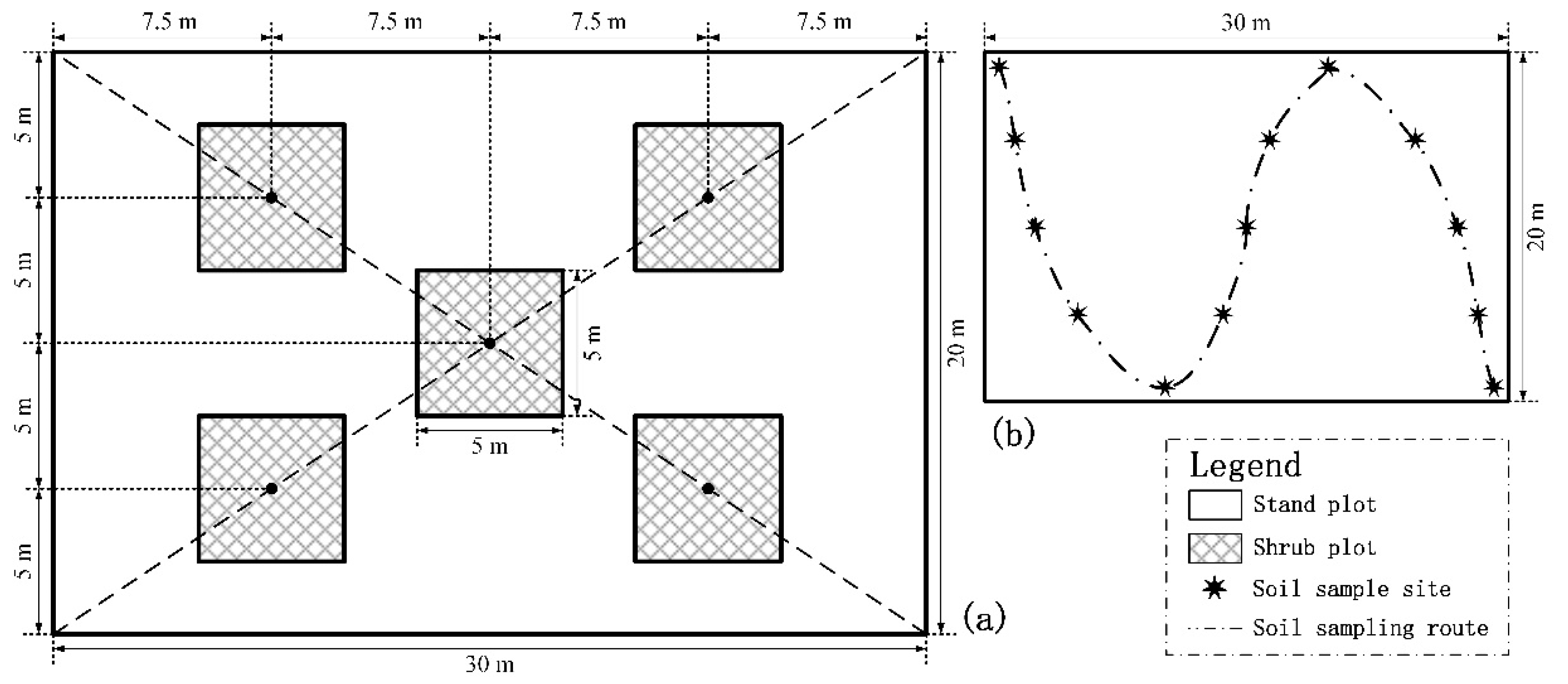
2.2. Forest Survey, Sample Collection, and Soil Sample Analysis

Fifty-seven 20 m × 30 m plots were delineated in a typical Chinese pine forest. In each plot, all trees with a diameter bigger than 3 cm at breast height were signed and recorded. Diameter at breast height (DBH) was measured using diameter tape, with 0.1 cm precision. The average slope and altitude were recorded using a portable GPS-G138BD (made by Unitstrong, Beijing, China). Litter thickness was measured on 1/4-point, 1/2-point, and 3/4-point across the diagonals, and canopy length was measured from north to south and east to west using a tape measure, with 0.1 m precision. Tree height was measured using a Blume-Leiss height indicator, with 0.5 m precision. Because our selected plots were in even-aged plantation forest, we used an increment borer to measure five different samples in each plot in order to determine the average age of the tree. The relative coordinates of trees in each plot were measured using a tape measure. To begin, each plot was first cut into a 5 m × 5 m grid; then each tree’s position within each grid was carefully determined. Canopy density was calculated based on the projection area of all canopy in a plot and total area of the plot, and this calculation was performed in ArcGIS 10.2 (Esri, Redlands, CA, USA). In addition, five shrub quadrats were designated within the 1/4-point, 1/2-point, and 3/4-point diagonals in the plots (Figure 1a). For each species in each shrub quadrat, we recorded shrub species, quantity, average height, and average coverage.
Soil samples from the 57 plots were collected from 10–12 August 2017 and 14–16 August 2018. Thirteen points were selected in each plot to form an S-shape (Figure 1b). Horizons of 0–30 cm were collected using a 5 cm diameter soil driller after the litter was removed. Soil samples collected at the same site were mixed into one sample. After removal of fine roots and the green vegetation parts, the soil samples were passed through a 2 mm sieve and stored at −4 °C for subsequent chemical and physical analyses. Soil bulk density samples were collected with a 100 mm2 cylindrical metal sampler.
The soil bulk density was gravimetrically determined via the soil-core method [18]. The SWC was measured by oven drying the soil at 105 °C until a constant weight was reached. Soil pH was measured in a 1:1 soil/KCl suspension using a Sartorius p-10 pH meter (Sartorius, Gottingen, Germany). The soil organic matter was assayed via the dichromate oxidation method [19]. The total nitrogen content was measured with a FOSS Kjeltec 8400 Analyzer Unit (FOSS, Hillerød, Denmark) using the Kjeldahl method [20]. The total phosphorus was digested by H2SO4-HClO4, then measured using a spectrophotometer [21]. Total carbon was measured from 1 mm sieved soil with a Liaui TOC II Analyzer (ELMENTAR, Langenselbold, Germany).

2.3. Variables

In this study, we used latent variables (i.e., variables that cannot be directly observed but are instead inferred from other observed variables) and observed variables to explain the relationship between various impact factors that pertain to shrub diversity (Table 1). Three independent latent variables (forest stand properties, site conditions and soil properties) and one dependent latent variable (shrub diversity) were selected to construct the PLS-SEM. The latent variable of forest stand properties was expounded upon using ten independent observed variables, including four spatial structure indexes—mingling (M) [22], dominance (U) [23], uniform angle index(W) [22,24], and crowding (C) [25] and six basic tree layer properties—forest stock volume (VOL), canopy density (CD), DBH, tree height (h), stand density (DEN), and average age of the tree (AGE). Due to the similarities of environmental condition in our plots, only three observed variables were chosen for explaining the latent variable of Site conditions—slope (SLO), litter thickness (LT), and altitude (ATT), which are considered microclimate driving factors. Moreover, to expound the latent soil property variable, soil organic matter (SOM), total carbon content (TC), total phosphorus content (TP), total nitrogen content (TN), soil bulk density (BD), soil water content (SWC), and pH were selected as the observed variables. To ensure the information dimensional integrity of latent variable of shrub diversity, five different diversity indexes which expressed in different information dimension and two shrub species properties were selected as observed variables to expound upon the dependent latent variable, including: total shrub species (S), total number of shrub (N), shrub layer Margalef index (MAR), shrub layer Pielon index (PIE), shrub layer Shannon-wiener index (SHA), shrub layer Simpson index (SIM), and shrub layer Gleason index (GLE).

2.4. Selection of Variables

In this study, we applied an RF algorithm to reduce the dependent latent variable redundancy and to eliminate the dependent observed variables that exhibit extremely low importance values [26]. RF is an ensemble method in which classification is performed by voting of multiple unbiased weak classifiers—decision trees [27]. The algorithm was performed by the “Boruta” package (R software ver-3.5.3), which provide the importance value to indicate whether a feature is vital by measure the loss of accuracy of classification caused by the random permutation of attribute values between objects though create a corresponding “shadow” attribute, whose values are obtained by shuffling values of the original attribute across objects [28].
Shrub layer diversity can be reflected by multiple diversity indexes which correlation show discrepancy with independent observed variables. Thus, we performed the RF algorithm to select diversity indexes more relevant to independent observed variable. Twenty independent observed variables were used to calculate the importance values of seven diversity indexes, respectively. Each independent observed variable was classified by seven diversity indexes, in order to obtain an importance values in one classification. Then, summarized the results of each importance value, the diversity indexes were voted in if it showed statistical significance in one classification. This voting was implemented to select diversity indexes that have greater relevant and criticality. RF and voting results were used as the input parameters, which support the dependent latent variables in the PLS-SEM model. In this work, the confidence level and maximum parameter RF algorithm runs were defined as 0.01 and 100, respectively.

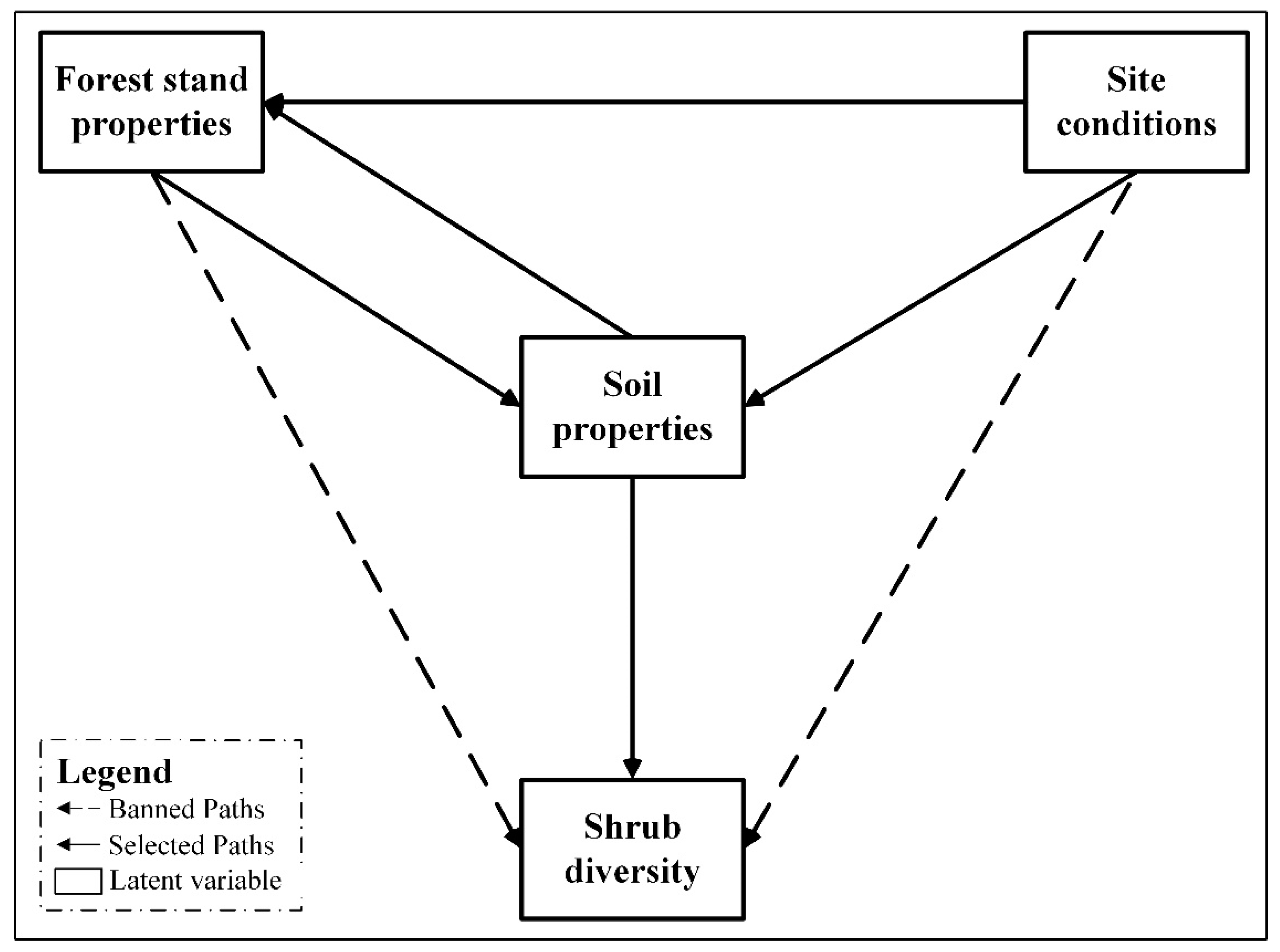
2.5. Establishment of Preliminary Model and Determination of Paths

SEM is a stochastic method that is employed to analyze and estimate the causal relationship between variable [29], contained factor analysis, and path analysis. It is mainly applied in the PLS-SEM and Covariance-Based Structural Equation Modeling (CB-SEM), etc. The PLS-SEM methid has better predictive accuracy when compared to CB-SEM, which focuses on parameter assessment [30]. In exploratory research, if little about the relationship among the variables is known, PLS-SEM, not CB-SEM, should be considered [31]. Furthermore, certain researchers also emphasize that PLS-SEM has a wider tolerance than CB-SEM, when sample size is limited and data are not normally distributed [32,33]. Therefore, a PLS-SEM was selected for this study.
The preliminary model was established based on the following causal assumptions: (1) the latent variables of site condition, forest stand properties, and soil properties directly impacted the latent variable of shrub diversity; (2) the latent variable of site condition indirectly impacted the latent variable of shrub diversity via the latent variables of forest stand properties and soil properties; and (3) the latent variable of forest stand properties indirectly impacted the latent variable of shrub diversity via the latent variable of soil properties (Figure 2).
To reduce the uncertainty in PLS-SEM running, the correlation relationship among the different groups of observed variables are examined. We performed a direct ordination analysis in each pair of groups of variables using the Canonical Correspondence Analysis (CCA). CCA is a direct gradient analysis method that explores the relationships between two groups of variables. The 20 independent observed variables and five dependent observed variables (diversity indexes, selected using the RF algorithm), were divided into four groups along four different latent variables. Then, six pairs of CCA were performed between the two groups for each variable. By verifying the significance of the six pairs using CCA, some paths in the preliminary model (Figure 2), which showed little significance, were excluded and potential paths in a secondary PLS-SEM model were confirmed. The CCA was performed using the “Vegan” package (R software ver-3.5.3).

2.6. Evaluation of PLS-SEM

Based on the results of RF and CCA, we performed and estimated factor analysis and path analysis in PLS-SEM. In the final PLS-SEM model’s construct reliability and inner model validity were evaluated using the Composite Reliability value (CR) and the Average Variance Extracted value (AVE). A CR value > 0.7 indicates good internal consistency and reliability [34]; while an AVE value > 0.5 indicates good-fitting, convergent validity [35]. The discriminant validity should be evaluated by a matrix that follows the Fornell-Larcker Criterion. The square root of the AVE of a reflected latent variable should be larger than the correlation coefficient values with other latent variables [35]. Variance Inflation Factor values (VIFs) were examined to avoid multicollinearity of observed variables, as only one variable from each pair of significantly correlated variables was used. The VIF of each variable should be <5.0 [36]. To avoid model misspecification, Henseler introduced the Standardized Root Mean Square Residual value (SRMR) as a goodness fit measure for the PLS-SEM [37]. The SRMR value should be <0.10 [38]. In the PLS-SEM, a bootstrapping procedure was applied in order to obtain T-statistics for the structural path’s significance testing. The p-value of the T-statistics should be <0.05 (or the T-statistics should be >1.96), which indicates that the path coefficient is significant [31]. In this work, the maximum PLS algorithm iterations were set at 5000 times. The stop criterion is a threshold value that should be smaller than the difference of outer weight and is therefore set to 10−7 in the PLS algorithm. In addition, we set the bootstrapping subsamples as 10,000 and the bootstrapping significance level at 0.05 to ensure the reliability. All of the PLS-SEM statistical analyses were performed using SmartPLS 3 (ver-3.2.8, SmartPLS GmbH, Boenningstedt, Germany).

3. Results

One hundred and five shrub species and 14,321 individual shrub plants were observed in our 57 plots. Lonicera maackii, which was observed in 53 plots, was the most common shrub in the study area, followed by Celastrus orbiculatus, Vitaceae ampelopsis, and Euonymus alatus, which were observed in 48, 42, and 40 of the plots, respectively. The seven dependent observed variables, which were used to explain the latent variables of shrub diversity ranged from: S: 9–26, N: 29–500, MAR: 1.54–4.60, PLE: 0.41–0.90, SHA: 1.18–2.68, SIM: 0.54–0.90, and GLE: 1.04–5.38 based on our 57 plots, respectively.

3.1. Observed Variables of Latent Variables of Shrub Diversity

In the RF algorithm, the seven dependent observed variables were classified by each of the 20 independent observed variables that belonged to the latent variables of forest stand properties, site conditions, and soil properties. The contribution of dependent observed variables to independent ones was recognized as the importance value. Based on these regressions, we obtained 20 groups of importance values (Figure 3). The importance values in the VOL, CD, and TP groups showed the best acceptance level, with only one importance value rejected from each group. The PIE was rejected from groups VOL and CD, which depicted importance values of 1.87 and −0.37, respectively; while N was rejected from group TP, due to its importance value being −3.07. SLO, h, PH, BD and TN all depicted the minimum acceptance level, and therefore all variables in these groups were rejected. 8, 24, and 17 importance values were received from different observed variables belonging to latent variables of site conditions, forest stand properties, and soil properties, respectively.
We ranked the seven dependent observed variables using a total of 49 received importance values (Figure 3). Results, in decreasing order, are as follows: N and MAR (ten votes each) >SIM, SHA, and GLE (seven votes each) >S (five votes) >PIE (three votes). The votes for N and SHA are basically from two latent variables. N received all the votes from the latent variable of forest stand properties, excepting U and h, as well as two votes from the latent variable of site condition; while the latent variable of forest stand properties and soil properties contributed three and four votes to SHA, respectively. Only the observed variables of TP, SWC, and TC from the latent variable of soil properties contributed three votes to PIE, which received the least votes in the seven dependent observed variables. MAR, SIM, GLE and S received votes from each of the three latent variables. Based on the total number and distribution of votes for each dependent observed variable, five variables—N, MAR, SIM, SHA and GLE—were selected as the observed variables for the shrub diversity latent variable in the PLS-SEM.

3.2. Possible Path and Model

The CCA results of site condition vs. shrub diversity and forest stand properties vs. shrub diversity was not statistically significant. These may due to the site environment and tree layers having little relevant direct effect on the latent variable of shrub diversity. The results of site condition vs. forest stand properties, site conditions vs. soil properties, and forest stand properties vs. soil properties were statistically highly significant. These results conform to the interaction among tree layers, soil layers, and environmental factors. In addition, the CCA result for soil property vs. shrub diversity showed a significant correlation relationship, indicating that the soil layer may have a strong connection with shrub layer diversity (Table 2).
If the CCA result was not significant between two groups of variables, we concluded that there were no potential paths between this pair of latent variables in PLS-SEM (an observed variables group was recognized as a latent variable in SEM). Thus, based on CCA results for different pairs of variables groups, the preliminary PLS-SEM model was adjusted by excluding two paths— from the latent variable of forest stand properties to the latent variable of shrub diversity and from the latent variable of site conditions to the latent variable of shrub diversity. Figure 4 depicts the proposed potential secondary model.

3.3. Model Fit

The best fit model is illustrated in Figure 5. In the best fit model, the CR valued 0.839, indicating the model demonstrates good internal consistency and reliability; while an AVE of 0.667 shows good-fitting convergent validity of our final model. The discriminant validity was evaluated using a Fornell-Larcker criterion matrix. In this matrix, the AVE square root of the latent variable of shrub diversity was 0.816; which is larger than its correlation coefficient value with other latent variables. To avoid multicollinearity of observed variables, a VIF statistical analysis was performed on the objective variables. All variable VIFs were <3.0 except GLE (VIF = 4.7) and MAR (VIF = 5.0), which were reluctantly accepted in the final hypothesis. As a goodness fit measure for the PLS-SEM, the SRMR value of 0.099 is acceptable.

3.4. Evaluation of Shrub Diversity’s Effect Factor

The final model’s factor analysis in SEM showed the weight of each observed variable relative to the latent variables (Figure 5). The weight of MAR and GLE is 0.497 and 0.519, respectively; which means they are responsible for 96.2% of the contribution to the latent variable of shrub diversity. For latent variables of site conditions, the weight of ATT and LT is 0.772 and 0.448, respectively. The SWC observed variable made the most considerable contribution to the latent variable of soil properties with a weight value of 0.666, while SOM contributed the least with a weight of 0.059. C and AGE had a negative effect on the latent variable of forest stand properties, with weights of −0.235 and −0.941, respectively. In turn, DBH, W and VOL had a positive effect, depicting weight values of 0.778, 0.533 and 0.795, respectively.
Based on the bootstrapping results, the T-statistics and p-value of all three paths are acceptable, which means the final model’s three total effects are significant (Figure 5). The total effects of the latent variable of site conditions to the latent variable of soil properties (T-statistics = 3.919, p-value < 0.001), the latent variable of soil properties to the latent variable of shrub diversity (T-statistics = 2.544, p-value < 0.05), and the latent variable of forest stand properties to the latent variable of soil properties (T-statistics = 2.147, p-value < 0.05) is 0.514, 0.344 and 0.326, respectively. Moreover, the indirect effect of the latent variable of site conditions to the latent variable of shrub diversity is 0.177 (T-statistics = 1.978, p-value < 0.05), which is accepted based on the bootstrapping result. However, the indirect effect of the latent variable of forest stand properties to the latent variable of shrub diversity was not significant (indirect effect = 0.112, T-statistics = 1.481, p-value > 0.05).

4. Discussion

4.1. Direct Effect of Shrub Diversity

In this study, we quantified and evaluated the direct impact of shrub diversity. Our results highlight that the latent variable of shrub diversity was mainly influenced by a direct effect from the latent variable of soil properties. Similar results were reported in John et al. [7] which stated that belowground nutrient availability plays an essential role in plant distribution.
For the objective variables, our result demonstrated that SWC is a major contributor and was recognized as one of the factors that affect plant diversity [39]. This highest contribution from SWC was mainly due to our study area being located in the Loess Plateau, where SWC was restricted by limited precipitation and soil erosion [40]. Li et al. [41] also reported that shrub species richness and abundance were mainly determined by SWC. Total nitrogen was recognized as another major variable that determines the composition and diversity of vegetation, in that nitrogen concentration has a negative effect on plant diversity [42]. Furthermore, our results show that total soil phosphorus is also vital for the latent variable of shrub diversity. These results are in agreement with Condit et al. [43] who reported that phosphorus is the strongest predictor of more than half of the plant distribution in the tropical forest. Furthermore, Zemunik et al. [44] reported that phosphorus’s key role is one of the vital factors that support the plant community. In this study, SOM contributes little to the latent variable of shrub diversity, which conflicts with the results from Fu et al. [45] who reported that SOM has the largest effect on shrub richness and α-diversity. Yet, our results are in good agreement with Lu Nini [46] who reported that there is no statistically significant influence of SOM on the latent variable of shrub diversity. This phenomenon might be explained by the fact that the main tree species in our study and Lu’s study is conifer, while Fu’s research was primarily conducted on hardwood species. SOM in conifer forests has more lignin, which in turn generates lower activity than broad-leaves forests [47].

4.2. Site Condition Influence On Shrub Diversity as Demonstrated by the Effects on the Soil Properties

Our results show that the latent variable of site condition is directly influencing the latent variable of Soil properties and indirectly impacting the latent variable of shrub diversity (via its direct effect on soil), which indicated that no direct causal relationship between shrub diversity and environmental factors.
According to our results, the composition and distribution of the shrub layer are significantly influenced by observed variable of altitude. This result agrees with Chawla et al. [48] who reported that the relationship between altitude and plant diversity was depicted by a hump-shaped curve. A direct effect is identifiable in the latent variable of site conditions to the latent variable of soil properties. Altitude gradient has a significant influence on soil nutrition. Temperature and moisture, which are affected by altitude, may influence the availability of crucial plant nutrients [49]. Moreover, the lower temperature in high altitude areas limits the soil’s organic matter decomposition rate and microbial activity [50]. Litter thickness (LT) is another site condition key variable that directly influenced the latent variable of soil properties. Litter is recognized as an inherent part of nutrient cycling [51]. Significant differences in litter thickness may indicate different soil nitrite circulation. Long-term litter removal experiments demonstrated that TN concentration significantly decreased to about 40% and TP concentration decreased to 37% [52]. In addition, we also identified an indirect effect of LT on the latent variable of shrub diversity. Litter is defined as a protective layer on the soil surface that regulates microclimates. Small-scale microclimatic heterogeneity promotes species richness and diversity [53]. For example, results from a long-term study by Shaolin et al. [52] demonstrated increased diversity of herb and shrub layers in stands where the litter was not harvested.
In our study, the weight of ATT > LT. That may be because our plots drop from 1519 m to 1114 m, which facilitates a more significant environment index change (for example: soil temperature) than litter thickness variation. Meanwhile, litter decomposition is a very long process, which is also affected by altitude change. Thus, ATT contributed a stronger effect than LT.

4.3. Effect of Tree Layers on Soil Properties

Our results also highlight that there is no statistically significant effect between the latent variables of forest stand properties and shrub diversity—which conflicts with some previous studies [10,11]. Undeniably, there is a strong and visible relationship between some of the observed variables of the forest stand properties and the shrub diversity. For example, the forest spatial structural index of C, which indicates the canopy structure and the illumination input, has complex effects on the shrub layer’s distribution and composition [54]. However, this strong relationship was not depicted between latent variables of forest stand properties and shrub diversity, which may because observed variable C is only one part of the latent variable of forest stand properties and the latent variable of forest stand properties also expresses the information of other four observed variables. In addition, our plots were established in a plantation forest that exhibited a monotonous tree layer composition and the natural relationship between shrub layer and tree layer was highly interrupted by human activities. Therefore, unlike the results presented by Bergstedt and Milberg [11], in this study, tree layers may not be considered a main driving factor of shrub layer diversity.
However, our results show a statistically significant relationship between latent variables of soil properties and forest stand properties. Based on the factor analysis in PLS-SEM of the latent variable of forest stand structure, observed variable AGE was recognized as one of the main factors that impact soil properties. This result agrees with Guomei et al. [55], who found that total nitrogen content peaked in a secondary 17-year-old forest located in the north Ziwulin region of the Loess Plateau. Meanwhile, the weight of AGE is the largest recorded among other observed variables, which, in our study, is a latent variable of forest stand properties. It is because forest nutrition input and output rates are strongly affected by forest age-class. On one hand, a higher aged stand may allow a higher input of litter, which generally increases SOM content [56]. On the other hand, different soil nutrients may be absorbed at different rates in different forest periods and that may influence the soil elements’ distribution. Furthermore, our results concerning forest structure and soil properties are similar to Pötzelsberger and Hasenauer’s result, indicating that forest structure drives soil processes by alternative light, soil temperature, and moisture [57]. Our results showed that forest structure discrepancy may also induce a variation of soil elements and nutrition. Observed variables of C and W explained the distribution of canopy and trees in different stands. From one perspective, tree distribution has a strong correlation with plant root density, which in turn has a positive correlation with soil nitrogen and a negative correlation with soil moisture [58]. From another perspective, canopy and tree distribution decide the forms of canopy gap which recognized as an important factor that causes variant soil nutrient recycling processes by influencing temperature and moisture [59]. According to the results of Muscolo et al. [60], the highest temperature and moisture values were observed in a Pinus nigra forest with a large and small gap, respectively.
In our results, the weight of observed variable W is higher than C, which means the tree distribution contribution is more important than the canopy contribution. It is because the dominant tree species in our stands are Chinese pine, which possesses a strong root system. Furthermore, the Chinese pine is recognized as a table-shaped crown when mature [61]. Thus, the Chinese pine plantation forest’s canopy structure may have a minimal discrepancy, which in turn indicates lower contribution. The observed variables of DBH and VOL have similar impact on soil properties. Considerable evidence has shown that average DBH and forest stock volume have a significant relationship with root growth [62]. Root system changes may lead to alterations in soil element distribution in specific stands. Furthermore, root system modifications also have substantial influence on microorganisms, which significantly contributes to decomposition [50]. As a result, modification of soil element distribution and contents parallel increasing average DBH in a forest system.
Totally, our result indicated that environment and trees factors could influence shrub diversity via change soil properties and soil is the determinant of shrub diversity in a region scale area with Chinese pine plantation. However, tree layer factors, soil and environment may induce another complication in different scales of the forest ecosystem or in different ecosystems. Ideally, a far-ranging scale and more variables should be considered in a follow-up study.

5. Conclusions

Quantitative description of relationships among factors which could influence on shrub diversity is crucial for understanding the diversity in forest ecosystem and could provide new insights in plantation forest diversity research. In this work, we used a PLS-SEM to quantify the effect among these impact factors of the latent variable of shrub diversity in a Chinese pine plantation forest. Our result shows that: (1) Soil factors, which are controlled by tree layer and site conditions were recognized as the main impact factor on the latent variable of shrub diversity; (2) Tree layer has a limited effect on the latent variable of shrub diversity, regardless of the fact that some tree layer variables have a strong connection to it; and (3) The latent variable of site conditions affects the latent variable of shrub diversity by influencing soil factors. The results of relationships among these factors and shrub diversity help in researchers’ understanding of forest diversity change, which may be applied in future precise forest prediction model and allows more effective forest management strategies.

Author Contributions

Conceptualization, B.W. and Y.B.; Data curation, B.W., Y.B. and N.Q.; Formal analysis, B.W. and Y.B.; Funding acquisition, W.L. and P.Z.; Investigation, B.W., Y.L. and R.G.; Methodology, B.W., Y.B. and Y.L.; Project administration, W.L. and P.Y.; Resources, Y.L. and Y.Y.; Software, B.W., Y.B. and Y.L.; Supervision, W.L. and P.Z.; Validation, Y.B.; Visualization, B.W. and Y.B.; Writing—original draft, B.W.; Writing—review & editing, Y.B., Y.L., W.L., P.Z and Y.Y.

Funding

This work was supported by the National Key Research and Development Program of China, grant number: 2016YFD060020305 and the Shaanxi Forest Department, grant number: SHLY-2018-02.

Acknowledgments

We acknowledge the Department of Huanglongshan Forestry Service for permission to conduct research in local forest. We wish to acknowledge the Center for Ecological Forecasting and Global Change, Northwest A&F University, for providing laboratories for the soil experiment.

Conflicts of Interest

The funders had no role in the design of the study; in the collection, analyses, or interpretation of data; in the writing of the manuscript, or in the decision to publish the results.

References

  1. FAO. Global Forest Resources Assessment 2015: How are the World’s Forests Changing? Food and Agriculture Organization of United Nation: Rome, Italy, 2016. [Google Scholar]
  2. Kelty, M.J. The role of species mixtures in plantation forestry. For. Ecol. Manag. 2006, 233, 195–204. [Google Scholar] [CrossRef]
  3. Evans, J.; Turnbull, J.W. Plantation Forestry in the Tropics: The Role, Silviculture, and Use of Planted Forests for Industrial, Social, Environmental, and Agroforestry Purposes; Oxford University Press: Oxford, UK, 2004; p. 480. [Google Scholar]
  4. Gracia, M.; Montané, F.; Piqué, J.; Retana, J. Overstory structure and topographic gradients determining diversity and abundance of understory shrub species in temperate forests in central Pyrenees (NE Spain). For. Ecol. Manag. 2007, 242, 391–397. [Google Scholar] [CrossRef]
  5. De Groote, S.R.E.; Vanhellemont, M.; Baeten, L.; De Schrijver, A.; Martel, A.; Bonte, D.; Lens, L.; Verheyen, K. Tree species diversity indirectly affects nutrient cycling through the shrub layer and its high-quality litter. Plant Soil 2018, 427, 335–350. [Google Scholar] [CrossRef]
  6. Myers-Smith, I.H.; Forbes, B.C.; Wilmking, M.; Hallinger, M.; Lantz, T.; Blok, D.; Tape, K.D.; Macias-Fauria, M.; Sass-Klaassen, U.; Lévesque, E.; et al. Shrub expansion in tundra ecosystems: Dynamics, impacts and research priorities. Environ. Res. Lett. 2011, 6, 045509. [Google Scholar] [CrossRef]
  7. John, R.; Dalling, J.W.; Harms, K.E.; Yavitt, J.B.; Stallard, R.F.; Mirabello, M.; Hubbell, S.P.; Valencia, R.; Navarrete, H.; Vallejo, M.; et al. Soil nutrients influence spatial distributions of tropical tree species. Proc. Natl. Acad. Sci. USA 2007, 104, 864–869. [Google Scholar] [CrossRef] [Green Version]
  8. Small, C.J.; McCarthy, B.C. Spatial and temporal variability of herbaceous vegetation in an eastern deciduous forest. Plant Ecol. 2003, 164, 37–48. [Google Scholar] [CrossRef]
  9. Grandin, U. Dynamics of understory vegetation in boreal forests: Experiences from Swedish integrated monitoring sites. For. Ecol. Manag. 2004, 195, 45–55. [Google Scholar] [CrossRef]
  10. Légaré, S.; Bergeron, Y.; Paré, D. Influence of Forest Composition on Understory Cover in Boreal Mixedwood Forests of Western Quebec. Silva Fennica 2002, 36, 353–366. [Google Scholar] [CrossRef]
  11. Bergstedt, J.; Milberg, P. The impact of logging intensity on field-layer vegetation in Swedish boreal forests. For. Ecol. Manag. 2001, 154, 105–115. [Google Scholar] [CrossRef]
  12. Frelich, L.E.; Machado, J.-L.; Reich, P.B. Fine-scale environmental variation and structure of understorey plant communities in two old-growth pine forests. J. Ecol. 2003, 91, 283–293. [Google Scholar] [CrossRef]
  13. Légaré, S.; Bergeron, Y.; Leduc, A.; Paré, D. Comparison of the understory vegetation in boreal forest types of southwest Quebec. Can. J. Bot. 2001, 79, 1019–1027. [Google Scholar] [CrossRef]
  14. Shi, Y.; Xu, L.; Zhou, Y.; Ji, B.; Zhou, G.; Fang, H.; Yin, J.; Deng, X. Quantifying driving factors of vegetation carbon stocks of Moso bamboo forests using machine learning algorithm combined with structural equation model. For. Ecol. Manag. 2018, 429, 406–413. [Google Scholar] [CrossRef]
  15. Granados-Peláez, C.; Santibáñez-Andrade, G.; Guerra-Martínez, F.; Serrano-Giné, D.; García-Romero, A. Evaluation of multi-causal dynamics of variability composition of patch edges in temperate forest. For. Ecol. Manag. 2018, 429, 207–216. [Google Scholar] [CrossRef]
  16. Tin Kam, H. Random decision forests. In Proceedings of the 3rd International Conference on Document Analysis and Recognition, Montreal, QC, Canada, 14–16 August 1995; pp. 278–282. [Google Scholar]
  17. Kaplan, D. Structural Equation Modeling: Foundations and Extensions; Sage Publications: Thousand Oaks, CA, USA, 2008; Volume 10. [Google Scholar]
  18. Van Groenewoud, H. Methods and samplers for obtaining undisturbed soil samples in the forest. METHODS 1960, 90, 272–274. [Google Scholar] [CrossRef]
  19. Walkley, A.; Black, I.A. An examination of the Degtjareff method for determining soil organic matter, and a proposed modification of the chromic acid titration method. Soil Sci. 1934, 37, 29–38. [Google Scholar] [CrossRef]
  20. Bremner, J.M. Nitrogen-total. In Methods of Soil Analysis, Part3; American Society of Agronomy-Soil Science Society of America: Madison, WI, USA, 1996; pp. 1085–1121. [Google Scholar]
  21. Parkinson, J.A.; Allen, S.E. A wet oxidation procedure suitable for the determination of nitrogen and mineral nutrients in biological material. Commun. Soil Sci. Plant Anal. 1975, 6, 1–11. [Google Scholar] [CrossRef]
  22. Gadow, K.V.; Huy, G.Y.; Albert, M. The uniform angle index—A structural parameter for describing tree distribution in forest stands. Forstwesen 1998, 115, 1–10. [Google Scholar]
  23. Hui, G.Y.; Albert, M.; Von Gadow, K. The measure of neighbourhood dimensions as a parameter to reproduce stand structures. Forstwiss. Cent. Bl. 1998, 117, 258–266. [Google Scholar] [CrossRef]
  24. Hui, G.; Gadow, K.V. The uniform angle index. Derivation of the optimal standard angle. Allg. Forst-U. J.-Ztg. 2002, 173, 173–177. [Google Scholar]
  25. Hu, Y.; Hui, G. How to describe the crowding degree of trees based on the relationship of neighboring trees. J. Beijing For. Univ 2015, 37, 1–8. [Google Scholar]
  26. Tuv, E.; Borisov, A.; Runger, G.; Torkkola, K. Feature selection with ensembles, artificial variables, and redundancy elimination. J. Mach. Learn. Res. 2009, 10, 1341–1366. [Google Scholar]
  27. Breiman, L. Random Forests. Mach. Learn. 2001, 45, 5–32. [Google Scholar] [CrossRef] [Green Version]
  28. Kursa, M.B.; Rudnicki, W.R. Feature selection with the Boruta package. J. Stat. Softw. 2010, 36, 1–13. [Google Scholar] [CrossRef]
  29. Doncaster, C.P. Structural Equation Modeling and Natural Systems; Grace, J.B., Ed.; Cambridge University Press: Cambridge, UK, 2006; pp. 368–369. [Google Scholar]
  30. Samani, S. Steps in Research Process (Partial Least Square of Structural Equation Modeling (PLS-SEM) A Review). Int. J. Soc. Sci. Bus. 2016, 1, 55–66. [Google Scholar]
  31. Wong, K.K.-K. Partial least squares structural equation modeling (PLS-SEM) techniques using SmartPLS. Mark. Bull. 2013, 24, 1–32. [Google Scholar]
  32. Bacon, L.D. Using LISREL and PLS to measure customer satisfaction. In Proceedings of the Sawtooth Software Conference Proceedings, La Jolla, CA, USA, 2–5 February 1999; pp. 305–306. [Google Scholar]
  33. Wong, K. Handling small survey sample size and skewed dataset with partial least square path modelling. Vue Mag. Mark. Res. Intell. Assoc. Novemb. 2010, 20, 20–23. [Google Scholar]
  34. Hair, J.F.; Anderson, R.E.; Tatham, R.L.; Black, W.C. Multivariate Data Analysis, 5th ed.; Prentice Hall: New York, NY, USA, 1998. [Google Scholar]
  35. Fornell, C.; Larcker, D.F. Evaluating Structural Equation Models with Unobservable Variables and Measurement Error. J. Mark. Res. 1981, 18, 39–50. [Google Scholar] [CrossRef]
  36. Hair, J.F.; Sarstedt, M. PLS-SEM: Indeed a Silver Bullet. J. Mark. Theory Pract. 2011, 19, 139–152. [Google Scholar] [CrossRef]
  37. Henseler, J.; Dijkstra, T.K.; Sarstedt, M.; Ringle, C.M.; Diamantopoulos, A.; Straub, D.W.; Ketchen, D.J.; Hair, J.F.; Hult, G.T.M.; Calantone, R.J. Common Beliefs and Reality About PLS:Comments on Rönkkö and Evermann (2013). Organ. Res. Methods 2014, 17, 182–209. [Google Scholar] [CrossRef]
  38. Hu, L.t.; Bentler, P.M. Cutoff criteria for fit indexes in covariance structure analysis: Conventional criteria versus new alternatives. Struct. Equ. Model. A Multidiscip. J. 1999, 6, 1–55. [Google Scholar] [CrossRef]
  39. Sang, W. Plant diversity patterns and their relationships with soil and climatic factors along an altitudinal gradient in the middle Tianshan Mountain area, Xinjiang, China. Ecol. Res. 2009, 24, 303–314. [Google Scholar] [CrossRef]
  40. Jia, X.; Shao, M.A.; Zhu, Y.; Luo, Y. Soil moisture decline due to afforestation across the Loess Plateau, China. J. Hydrol. 2017, 546, 113–122. [Google Scholar] [CrossRef]
  41. Li, X.; Tan, H.; He, M.; Wang, X.; Li, X. Patterns of shrub species richness and abundance in relation to environmental factors on the Alxa Plateau: Prerequisites for conserving shrub diversity in extreme arid desert regions. Sci. China Ser. D Earth Sci. 2009, 52, 669–680. [Google Scholar] [CrossRef]
  42. Goldberg, D.E.; Miller, T.E. Effects of Different Resource Additions of Species Diversity in an Annual Plant Community. Ecology 1990, 71, 213–225. [Google Scholar] [CrossRef]
  43. Condit, R.; Engelbrecht, B.M.J.; Pino, D.; Pérez, R.; Turner, B.L. Species distributions in response to individual soil nutrients and seasonal drought across a community of tropical trees. Proc. Natl. Acad. Sci. USA 2013, 110, 5064–5068. [Google Scholar] [CrossRef] [PubMed] [Green Version]
  44. Zemunik, G.; Turner, B.L.; Lambers, H.; Laliberté, E. Increasing plant species diversity and extreme species turnover accompany declining soil fertility along a long-term chronosequence in a biodiversity hotspot. J. Ecol. 2016, 104, 792–805. [Google Scholar] [CrossRef]
  45. Fu, B.J.; Liu, S.L.; Ma, K.M.; Zhu, Y.G. Relationships between soil characteristics, topography and plant diversity in a heterogeneous deciduous broad-leaved forest near Beijing, China. Plant Soil 2004, 261, 47–54. [Google Scholar] [CrossRef]
  46. Lu, N.N.; Gao, Z.X.; Zhang, P.; Xu, X.L.; Wang, X.J. Path Analysis between Soil Properties and Undergrowth Vegetation in Pure Chinese Fir Forest. J. Northeast For. Univ. 2015, 43, 73–77. [Google Scholar]
  47. Cleve, K.V.; Oliver, L.; Schlentner, R.; Viereck, L.A.; Dyrness, C.T. Productivity and nutrient cycling in taiga forest ecosystems. Can. J. For. Res. 1983, 13, 747–766. [Google Scholar] [CrossRef]
  48. Chawla, A.; Rajkumar, S.; Singh, K.N.; Lal, B.; Singh, R.D.; Thukral, A.K. Plant Species Diversity along an Altitudinal Gradient of Bhabha Valley in Western Himalaya. J. Mt. Sci. 2008, 5, 157–177. [Google Scholar] [CrossRef]
  49. Unger, M.; Leuschner, C.; Homeier, J. Variability of indices of macronutrient availability in soils at different spatial scales along an elevation transect in tropical moist forests (NE Ecuador). Plant Soil 2010, 336, 443–458. [Google Scholar] [CrossRef] [Green Version]
  50. Iii, F.S.C.; Matson, P.A.; Mooney, H.A. Principles of Terrestrial Ecosystem Ecology; Springer: New York, NY, USA, 2011. [Google Scholar]
  51. Sayer, E.J. Using experimental manipulation to assess the roles of leaf litter in the functioning of forest ecosystems. Biol. Rev. 2010, 81, 1–31. [Google Scholar] [CrossRef] [PubMed]
  52. Shaolin, P.; Hai, R.; Jianguo, W.; Hongfang, L. Effects of litter removal on plant species diversity: A case study in tropical Eucalyptus forest ecosystems in South China. J. Environ. Sci. 2003, 15, 367. [Google Scholar]
  53. Opedal, Ø.H.; Armbruster, W.S.; Graae, B.J. Linking small-scale topography with microclimate, plant species diversity and intra-specific trait variation in an alpine landscape. Plant Ecol. Divers. 2015, 8, 305–315. [Google Scholar] [CrossRef]
  54. Montgomery, R.A.; Chazdon, R.L. Forest structure, canopy architecture, and light transmittance in tropical wet forests. Ecology 2001, 82, 2707–2718. [Google Scholar] [CrossRef]
  55. Guomei, J.; Jing, C.; Chunyan, W.; Gang, W. Microbial biomass and nutrients in soil at the different stages of secondary forest succession in Ziwulin, northwest China. For. Ecol. Manag. 2005, 217, 117–125. [Google Scholar] [CrossRef]
  56. Högberg, M.N.; Chen, Y.; Högberg, P. Gross nitrogen mineralisation and fungi-to-bacteria ratios are negatively correlated in boreal forests. Biol. Fertil. Soils 2007, 44, 363–366. [Google Scholar] [CrossRef]
  57. Pötzelsberger, E.; Hasenauer, H. Forest–water dynamics within a mountainous catchment in Austria. Nat. Hazards 2015, 77, 625–644. [Google Scholar] [CrossRef]
  58. February, E.C.; Higgins, S.I. The distribution of tree and grass roots in savannas in relation to soil nitrogen and water. S. Afr. J. Bot. 2010, 76, 517–523. [Google Scholar] [CrossRef] [Green Version]
  59. Prescott, C.E. The influence of the forest canopy on nutrient cycling. Tree Physiol. 2002, 22, 1193. [Google Scholar] [CrossRef]
  60. Muscolo, A.; Sidari, M.; Mercurio, R. Influence of gap size on organic matter decomposition, microbial biomass and nutrient cycle in Calabrian pine (Pinus laricio, Poiret) stands. For. Ecol. Manag. 2007, 242, 412–418. [Google Scholar] [CrossRef]
  61. Li, H.; Zhao, J.; Zhou, C.; Merkle, S.A.; Zhang, J.-F. Morphologic characters and element content during development of Pinus tabuliformis seeds. J. For. Res. 2016, 27, 67–74. [Google Scholar] [CrossRef]
  62. Colin, F.; Drexhage, M. Estimating root system biomass from breast-height diameters. For. Int. J. For. Res. 2001, 74, 491–497. [Google Scholar] [CrossRef]
Figure 1. Shrub quadrats position (a) and the strategies of soil sampling (b).
Forests 10 00781 g001
Figure 2. Preliminary partial least squares structural equation model which shows the relationship between latent variables. The arrow indicates the effect between latent variables or weight of observed variables to latent variables. The rectangles indicate the latent variables; the ovals indicate the observed variables. ATT, altitude; LT, litter thickness; SLO, slope; SOM, soil organic matter; TP, total phosphorus content; TC, total carbon content; SWC, soil water content; pH, power of hydrogen; TN, total nitrogen content; BD, bulk density; DBH, diameter at breast height; C, Crowding index; U, Dominance index; M, Mingling index; W, Uniform angle index; CD, canopy density; h, tree height; DEN, stand density; AGE, average age of the tree; VOL, forest stock volume; S, total shrub species, N, total number of individual shrub; MAR, Margalef index, PIE, Pielon index, SHA, Shannon-wiener index; SIM, Simpson index; GLE, Gleason index.
Forests 10 00781 g002
Figure 3. Factor significance by Random Forest algorithm, * indicate the significance of independent observed variables which selected by dependent observed variables. TN, total nitrogen content; TP, total phosphorus content; BD, bulk density; SWC, soil water content; PH, power of hydrogen; TC, total carbon content; SOM, soil organic matter; C, crowding index; U, dominance index; M, mingling index; W, uniform angle index; AGE, average age of the tree; DEN, stand density; h, tree height; DBH, diameter at breast height; CD, canopy density; VOL, forest stock volume; ATT, altitude; LT, litter thickness; SLO, slope; S, total shrub species, N, total number of individual shrub; MAR, Margalef index, PIE, Pielon index, SHA, Shannon-Wiener index; SIM, Simpson index; GLE, Gleason index.
Forests 10 00781 g003
Figure 4. Secondary model based on CCA result.
Forests 10 00781 g004
Figure 5. Final best-fit model describing the relationship of latent variables and their observed variables. The thickness of the arrow indicates the effect between latent variables or weight of observed variables to latent variables. ATT, altitude; LT, litter thickness; SOM, soil organic matter; SWC, soil water content; TN, total nitrogen content; TP, total phosphorus content; C, crowding; DBH, diameter at breast height; W, Uniform angle index; AGE, average age of the tree; VOL, forest stock volume; GLE, Gleason index; MAR, Margalef index, SIM, Simpson index.
Forests 10 00781 g005
Table 1. Details of variables used in the research.
Latent VariableObserved VariableAbbreviationDetail
Forest stand propertiesminglingMThe mean fraction of trees among the k nearest neighbors of a given reference tree with heterospecific neighbors
dominanceUThe proportion of the n nearest neighbors of a given reference tree which are smaller than the reference tree
uniform angle indexWCharacterize the spatial distribution of a forest community or of individual tree species within that community by gradually comparing the included 4 angles with the standard angle
crowdingCCrowding degree of a neighborhood unit according to the overlapping of the crown in spatial micro-environment which clearly define the crowding degree for a reference tree and its four nearest neighbors
forest stock volumeVOLThe total volume of living trees in a stand that bigger than 3 m diameter at breast height
canopy densityCDThe aggregate of all vertically projected tree crowns onto the ground surface
diameter at breast heightDBHThe tree diameter measured at 1.3 m above the ground
tree heighthMean height of all the tree in a stand
stand densityDENthe number of stems on a per hectare basis in relative terms
average age of the treeAGEAverage age of all trees in a stand
Site conditionsslopeSLOMean angle of the site to the horizontal
litter thicknessLTMean thickness of litter in a stand
altitudeATTMean altitude of each plot
Soil propertysoil organic matterSOMThe content of organic matter component of soil
total carbon contentTCThe content of total carbon of soil
total phosphorus contentTPThe content of total phosphorus of soil
total nitrogen contentTNThe content of total nitrogen of soil
soil bulk densityBDThe weight of soil in a unit volume
soil water contentSWCThe content of water in soil
Pondus HydrogeniipHthe negative of the base 10 logarithm of the molar concentration of hydrogen ions in a solution
Shrub diversitytotal shrub speciesSTotal number of shrub species
total number of shrubsNTotal number of shrub individuals
Margalef species richness indexMAR MAR = S 1 lnN
Shannon diversity indexSHA SHA = p i lnp i and p i = N i N
Pielou’s evenness indexPIE PIE = N ( N 1 ) N i ( N i 1 )
Simpson diversity indexSIM SIM = 1 p i 2 and p i = N i N
Gleason richness indexGLE GLE = S lnA   A   is   the   area   of   each   plot
Table 2. The significance of paths between latent variables.
Latent Variables GroupCanonical Correlations 1p-ValueWilk’sChi-SQDF
Site conditions vs. forest stand properties0.6970.000 ★★★0.27363.66430
Site conditions vs. soil properties0.6990.000 ★★★0.29162.4221
Site conditions vs. shrub diversity0.5110.0720.63223.61912
Forest stand properties vs. soil properties0.8450.000 ★★★0.058134.0170
Forest stand properties vs. shrub diversity0.7680.0800.26064.64550
Soil properties vs. shrub diversity0.6420.020 0.33354.3635
★ indicates p < 0.05; ★★ indicates p < 0.01; ★★★ indicates p < 0.001.

