From Farms to Forests: Landscape Carbon Balance after 50 Years of Afforestation, Harvesting, and Prescribed Fire

Abstract
1. Introduction
2. Methods
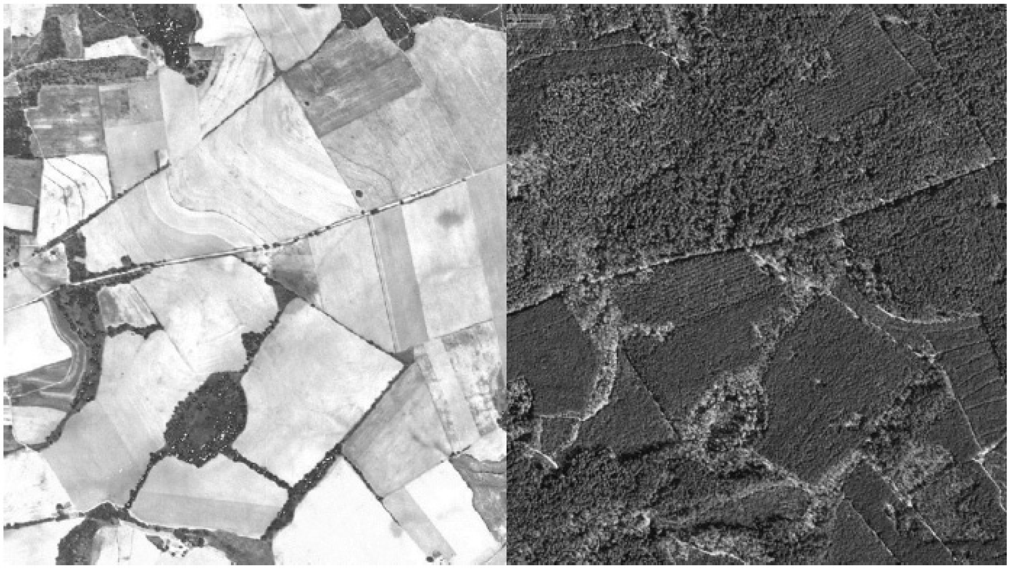
2.1. Study Area
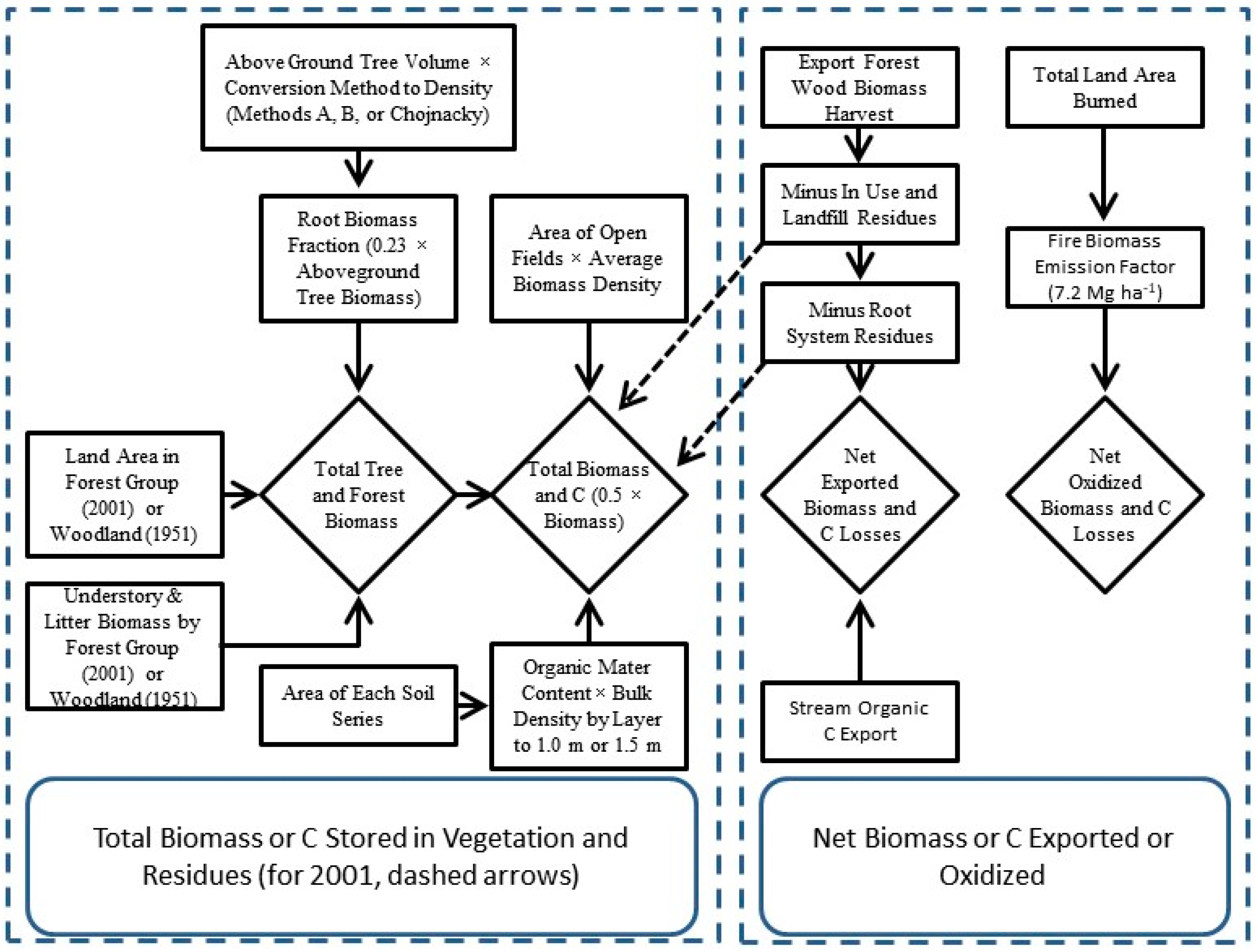
2.2. Estimates of Forest & Non-Forest Biomass
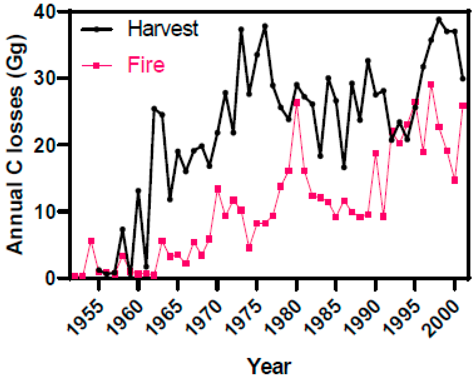
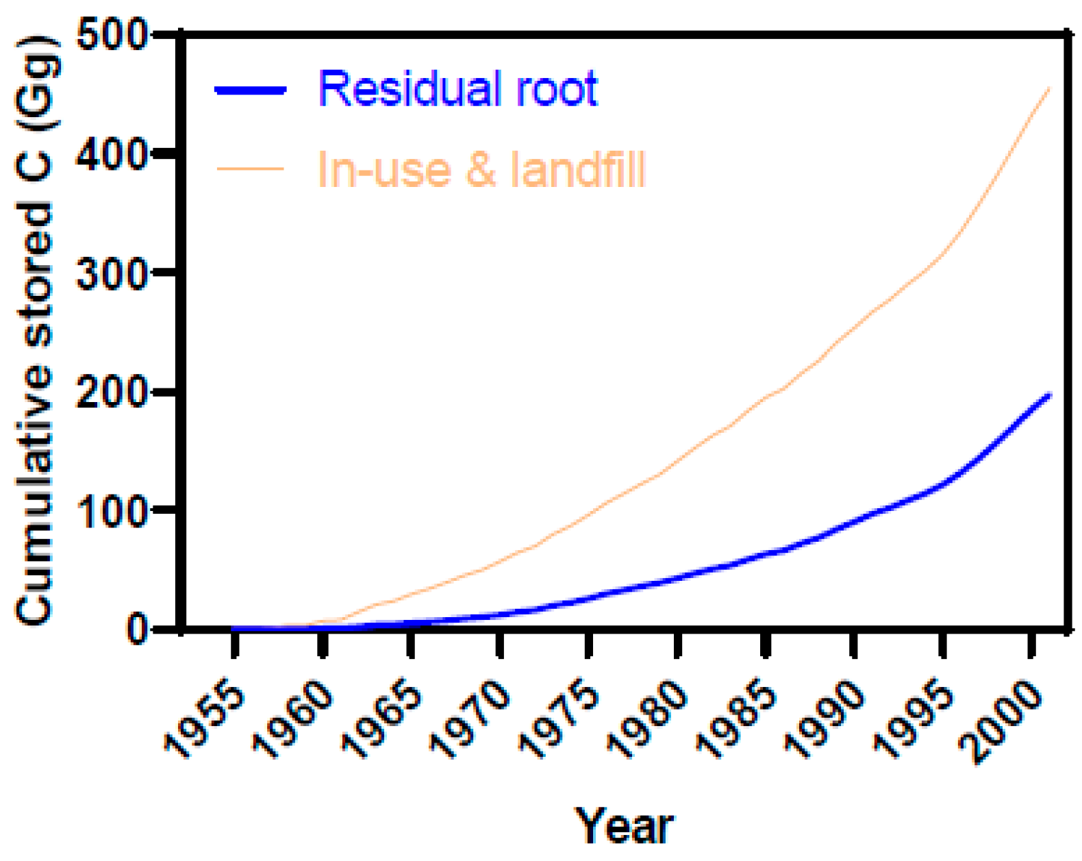
2.3. Estimates of Annual Biomass Fluxes, Life-Cycle Residues, and Net Ecosystem Production
2.4. Soil Organic Matter and Carbon
3. Results
3.1. Land Use Change
3.2. Estimates of Forest and Non-Forest Biomass
3.3. Estimates of Annual Carbon Fluxes and Life-Cycle Residues
3.4. Estimate of NBP between 1951 and 2001
3.5. Mineral Soil Carbon and Total C Stored in Vegetation and Soils in 2001
4. Discussion
4.1. Carbon Stocks & Fluxes after 50 Years of Afforestation
4.2. Comparison of Methodological Approaches
4.3. Soil Organic Carbon
5. Conclusions
Supplementary Materials
Author Contributions
Funding
Acknowledgments
Conflicts of Interest
References
- Birdsey, R.A.; Lewis, G. Carbon in US Forests and Wood Products, 1987–1997: State-by-State Estimates; Diane Publishing: Collingdale, PA, USA, 2003; Volume 310. [Google Scholar]
- Wear, D.N.; Greis, J.G. Southern Forest Resource Assessment-Technical Report; Gen. Tech. Rep. SRS-53; US Department of Agriculture, Forest Service, Southern Research Station: Asheville, NC, USA, 2002; Volume 53, 635p.
- Coulston, J.W.; Wear, D.N.; Vose, J.M. Complex forest dynamics indicate potential for slowing carbon accumulation in the southeastern United States. Sci. Rep. 2015, 5, 8002. [Google Scholar] [CrossRef] [PubMed]
- Zhao, S.Q.; Liu, S.G.; Sohl, T.; Young, C.; Werner, J. Land use and carbon dynamics in the southeastern United States from 1992 to 2050. Environ. Res. Lett. 2013, 8, 044022. [Google Scholar] [CrossRef]
- U.S. Forest Service. US Forest Facts and Historical Trends; USDA Forest Service: Washington, DC, USA, 2000.
- Hoefnagels, R.; Junginger, M.; Faaij, A. The economic potential of wood pellet production from alternative, low-value wood sources in the southeast of the US. Biomass Bioenergy 2014, 71, 443–454. [Google Scholar] [CrossRef]
- Martin, K.L.; Hurteau, M.D.; Hungate, B.A.; Koch, G.W.; North, M.P. Carbon Tradeoffs of Restoration and Provision of Endangered Species Habitat in a Fire-Maintained Forest. Ecosystems 2015, 18, 76–88. [Google Scholar] [CrossRef]
- Griffiths, N.A.; Rau, B.M.; Vache, K.B.; Starr, G.; Bitew, M.M.; Aubrey, D.P.; Martin, J.A.; Benton, E.; Jackson, C.R. Environmental effects of short-rotation woody crops for bioenergy: What is and isn’t known. Glob. Chang. Biol. Bioenergy 2019, 11, 554–572. [Google Scholar] [CrossRef]
- Kline, K.L.; Coleman, M.D. Woody energy crops in the southeastern United States: Two centuries of practitioner experience. Biomass Bioenergy 2010, 34, 1655–1666. [Google Scholar] [CrossRef]
- Popp, J.; Lakner, Z.; Harangi-Rakos, M.; Fari, M. The effect of bioenergy expansion: Food, energy, and environment. Renew. Sustain. Energy Rev. 2014, 32, 559–578. [Google Scholar] [CrossRef]
- Soussana, J.F.; Lutfalla, S.; Ehrhardt, F.; Rosenstock, T.; Lamanna, C.; Havlik, P.; Richards, M.; Wollenberg, E.; Chotte, J.L.; Torquebiau, E.; et al. Matching policy and science: Rationale for the ‘4 per 1000-soils for food security and climate’ initiative. Soil Tillage Res. 2019, 188, 3–15. [Google Scholar] [CrossRef]
- Wills, S.; Loecke, T.; Sequeira, C.; Teachman, G.; Grunwald, S.; West, L.T. Overview of the US rapid carbon assessment project: Sampling design, initial summary and uncertainty estimates. In Soil Carbon; Springer: Berlin/Heidelberg, Germany, 2014; pp. 95–104. [Google Scholar]
- Johnsen, K.H.; Wear, D.; Oren, R.; Teskey, R.; Sanchez, F.; Will, R.; Butnor, J.; Markewitz, D.; Richter, D.; Rials, T. Carbon sequestration and southern pine forests. J. For. 2001, 99, 14–21. [Google Scholar]
- Sampson, D.A.; Wynne, R.H.; Seiler, J.R. Edaphic and climatic effects on forest stand development, net primary production, and net ecosystem productivity simulated for Coastal Plain loblolly pine in Virginia. J. Geophys. Res. Biogeosci. 2008, 113. [Google Scholar] [CrossRef]
- Galik, C.S.; Mobley, M.L.; Richter, D.D. A virtual “field test” of forest management carbon offset protocols: The influence of accounting. Mitig. Adapt. Strateg. Glob. Chang. 2009, 14, 677–690. [Google Scholar] [CrossRef]
- Nunery, J.S.; Keeton, W.S. Forest carbon storage in the northeastern United States: Net effects of harvesting frequency, post-harvest retention, and wood products. For. Ecol. Manag. 2010, 259, 1363–1375. [Google Scholar] [CrossRef]
- Wilkes, P.; Disney, M.; Vicari, M.B.; Calders, K.; Burt, A. Estimating urban above ground biomass with multi-scale LiDAR. Carbon Balance Manag. 2018, 13, 10. [Google Scholar] [CrossRef] [PubMed]
- Heath, L.S.; Smith, J.E.; Woodall, C.W.; Azuma, D.L.; Waddell, K.L. Carbon stocks on forestland of the United States, with emphasis on USDA Forest Service ownership. Ecosphere 2011, 2, 1–21. [Google Scholar] [CrossRef]
- Frank, D.; Reichstein, M.; Bahn, M.; Thonicke, K.; Frank, D.; Mahecha, M.D.; Smith, P.; Van der Velde, M.; Vicca, S.; Babst, F.; et al. Effects of climate extremes on the terrestrial carbon cycle: Concepts, processes and potential future impacts. Glob. Chang. Biol. 2015, 21, 2861–2880. [Google Scholar] [CrossRef] [PubMed]
- Thom, D.; Seidl, R. Natural disturbance impacts on ecosystem services and biodiversity in temperate and boreal forests. Biol. Rev. 2016, 91, 760–781. [Google Scholar] [CrossRef]
- Nave, L.E.; Swanston, C.W.; Mishra, U.; Nadelhoffer, K.J. Afforestation Effects on Soil Carbon Storage in the United States: A Synthesis. Soil Sci. Soc. Am. J. 2013, 77, 1035–1047. [Google Scholar] [CrossRef]
- Smith, J.E.; Heath, L.S.; Skog, K.E.; Birdsey, R.A. Methods for Calculating Forest Ecosystem and Harvested Carbon with Standard Estimates for Forest Types of the United States; Gen. Tech. Rep. NE-343; US Department of Agriculture, Forest Service, Northeastern Research Station: Newtown Square, PA, USA, 2006; Volume 343, p. 216.
- Mobley, M.L.; Lajtha, K.; Kramer, M.G.; Bacon, A.R.; Heine, P.R.; Richter, D.D. Surficial gains and subsoil losses of soil carbon and nitrogen during secondary forest development. Glob. Chang. Biol. 2015, 21, 986–996. [Google Scholar] [CrossRef]
- Wang, F.M.; Zhu, W.X.; Chen, H. Changes of soil C stocks and stability after 70-year afforestation in the Northeast USA. Plant Soil 2016, 401, 319–329. [Google Scholar] [CrossRef]
- Kilgo, J.C.; Blake, J.I. Ecology and Management of a Forested Landscape: Fifty Years on the Savannah River Site; Island Press: Washington, DC, USA, 2005. [Google Scholar]
- White, D.L. Deerskins and Cotton. Ecological Impacts of Historical Land Use in the Central Savannah River Area of the Southeastern US before 1950; USDA Forest Service, Savannah River: New Ellenton, SC, USA, 2004.
- IPCC. Climate Change 2007: The Physical Science Basis. Contribution of Working Group I to the Fourth Assessment Report of the Intergovernmental Panel on Climate Change; Cambridge University Press: New York, NY, USA, 2007. [Google Scholar]
- Parresol, B.R.; Scott, D.A.; Zarnoch, S.J.; Edwards, L.A.; Blake, J.I. Modeling forest site productivity using mapped geospatial attributes within a South Carolina Landscape, USA. For. Ecol. Manag. 2017, 406, 196–207. [Google Scholar] [CrossRef]
- Coyle, D.R.; Aubrey, D.P.; Coleman, M.D. Growth responses of narrow or broad site adapted tree species to a range of resource availability treatments after a full harvest rotation. For. Ecol. Manag. 2016, 362, 107–119. [Google Scholar] [CrossRef]
- Aubrey, D.P.; Coleman, M.D.; Coyle, D.R. Ice damage in loblolly pine: Understanding the factors that influence susceptibility. For. Sci. 2007, 53, 580–589. [Google Scholar]
- Aubrey, D.P.; Coyle, D.R.; Coleman, M.D. Functional groups show distinct differences in nitrogen cycling during early stand development: Implications for forest management. Plant Soil 2012, 351, 219–236. [Google Scholar] [CrossRef]
- Aubrey, D.P.; Fraedrich, S.W.; Harrington, T.C.; Olatinwo, R. Cristulariella moricola associated with foliar blight of Camden white gum (Eucalyptus benthamii), a bioenergy crop. Biomass Bioenergy 2017, 105, 464–469. [Google Scholar] [CrossRef]
- Birdsey, R.A. Carbon Storage and Accumulation in United States Forest Ecosystems; Gen. Tech. Rep. WO-59; US Department of Agriculture, Forest Service, Washington Office: Washington, DC, USA, 1992; Volume 59, p. 51.
- Smith, J.E.; Heath, L.S.; Jenkins, J.C. Forest Volume-to-Biomass Models and Estimates of Mass for Live and Standing Dead Trees of US Forests; Gen. Tech. Rep. NE-298; US Department of Agriculture, Forest Service, Northeastern Research Station: Newtown Square, PA, USA, 2003; Volume 298, p. 57.
- Jenkins, J.C.; Chojnacky, D.C.; Heath, L.S.; Birdsey, R.A. National-scale biomass estimators for United States tree species. For. Sci. 2003, 49, 12–35. [Google Scholar]
- Chojnacky, D.C.; Heath, L.S.; Jenkins, J.C. Updated generalized biomass equations for North American tree species. Forestry 2013, 87, 129–151. [Google Scholar] [CrossRef]
- Odum, E.P. Organic Production and Turnover in Old Field Succession. Ecology 1960, 41, 34–49. [Google Scholar] [CrossRef]
- Lovett, G.M.; Cole, J.J.; Pace, M.L. Is net ecosystem production equal to ecosystem carbon accumulation? Ecosystems 2006, 9, 152–155. [Google Scholar] [CrossRef]
- Ludovici, K.H.; Zarnoch, S.J.; Richter, D.D. Modeling in-situ pine root decomposition using data from a 60-year chronosequence. Can. J. For. Res. 2002, 32, 1675–1684. [Google Scholar] [CrossRef][Green Version]
- Odum, E.P.; Pinder, J.E.; Christiansen, T.A. Nutrient Losses from Sandy Soils during Old-Field Succession. Am. Midl. Nat. 1984, 111, 148–154. [Google Scholar] [CrossRef]
- Rogers, V.A. Soil Survey of Savannah River Plant Area, parts of Aiken, Barnwell, and Allendale Counties, South Carolina; USDA Soil Conservation Service: Washington, DC, USA, 1990.
- McCormack, J.F.; Cruikshank, J.W. South Carolina’s Forest Resources, 1947; Southeastern Forest Experiment Station: Asheville, NC, USA, 1949. [Google Scholar]
- Parresol, B.R.; Blake, J.I.; Thompson, A.J. Effects of overstory composition and prescribed fire on fuel loading across a heterogeneous managed landscape in the southeastern USA. For. Ecol. Manag. 2012, 273, 29–42. [Google Scholar] [CrossRef]
- Dixon, K.; Rogers, V.; Conner, S.; Cummings, C.; Gladden, J.; Weber, J. Geochemical and Physical Properties of Wetland Soils at the Savannah River Site; Westinghouse Savannah River Co.: Aiken, SC, USA, 1996. [Google Scholar]
- Brudvig, L.A.; Grman, E.; Habeck, C.W.; Orrock, J.L.; Ledvina, J.A. Strong legacy of agricultural land use on soils and understory plant communities in longleaf pine woodlands. For. Ecol. Manag. 2013, 310, 944–955. [Google Scholar] [CrossRef]
- Tian, H.Q.; Chen, G.S.; Zhang, C.; Liu, M.L.; Sun, G.; Chappelka, A.; Ren, W.; Xu, X.F.; Lu, C.Q.; Pan, S.F.; et al. Century-Scale Responses of Ecosystem Carbon Storage and Flux to Multiple Environmental Changes in the Southern United States. Ecosystems 2012, 15, 674–694. [Google Scholar] [CrossRef]
- Hu, H.F.; Wang, G.G. Changes in forest biomass carbon storage in the South Carolina Piedmont between 1936 and 2005. For. Ecol. Manag. 2008, 255, 1400–1408. [Google Scholar] [CrossRef]
- Spinney, M.P.; Van Deusen, P.C.; Heath, L.S.; Smith, J.E. COLE: Carbon On-line Estimator, Version 2. In Changing Forests-Challenging Times, Proceedings of the New England Society of American Foresters 85th Winter Meeting, Portland, Maine, 16–18 March 2005; Kenefic, L.S., Twery, M.J., Eds.; Gen. Tech. Rep. NE-325; US Department of Agriculture, Forest Service, Northeastern Research Station: Newtown Square, PA, USA, 2005; p. 28. [Google Scholar]
- Woodbury, P.B.; Smith, J.E.; Heath, L.S. Carbon sequestration in the US forest sector from 1990 to 2010. For. Ecol. Manag. 2007, 241, 14–27. [Google Scholar] [CrossRef]
- Pregitzer, K.S.; Euskirchen, E.S. Carbon cycling and storage in world forests: Biome patterns related to forest age. Glob. Chang. Biol. 2004, 10, 2052–2077. [Google Scholar] [CrossRef]
- Dosskey, M.G.; Bertsch, P.M. Forest Sources and Pathways of Organic-Matter Transport to a Blackwater Stream—A Hydrologic Approach. Biogeochemistry 1994, 24, 1–19. [Google Scholar] [CrossRef]
- Smith, J.E.; Heath, L.S. A Model of Forest Floor Carbon Mass for United States Forest Types; Res. Pap. NE-722; US Department of Agriculture, Forest Service, Northeastern Research Station: Newtown Square, PA, USA, 2002; Volume 722, p. 37.
- U.S. Department of Energy. Natural Resources Plan for the Savannah River Site; USDA Forest Service-Savannah River: New Ellenton, SC, USA, 2005.
- Andreu, A.; Crolley, W.; Paresol, B. Analysis of Inventory Data Derived Fuel Characteristics and Fire Behavior under Various Environmental Conditions; USDA Forest Service-Savannah River: New Ellenton, SC, USA, 2013.
- Domke, G.M.; Perry, C.H.; Walters, B.F.; Woodall, C.W.; Russell, M.B.; Smith, J.E. Estimating litter carbon stocks on forest land in the United States. Sci. Total Environ. 2016, 557, 469–478. [Google Scholar] [CrossRef]
- Chang, C.-T.; Wang, C.-P.; Chou, C.-Z.; Duh, C.-T. The importance of litter biomass in estimating soil organic carbon pools in natural forests of Taiwan. Taiwan J. For. Sci. 2010, 25, 171–180. [Google Scholar]
- Zarnoch, S.J.; Blake, J.I.; Parresol, B.R. Are prescribed fire and thinning dominant processes affecting snag occurrence at a landscape scale? For. Ecol. Manag. 2014, 331, 144–152. [Google Scholar] [CrossRef]
- Samuelson, L.J.; Stokes, T.A.; Butnor, J.R.; Johnsen, K.H.; Gonzalez-Benecke, C.A.; Martin, T.A.; Cropper, W.P., Jr.; Anderson, P.H.; Ramirez, M.R.; Lewis, J.C. Ecosystem carbon density and allocation across a chronosequence of longleaf pine forests. Ecol. Appl. 2017, 27, 244–259. [Google Scholar] [CrossRef] [PubMed]
- Wijewardane, N.K.; Ge, Y.; Wills, S.; Loecke, T. Prediction of soil carbon in the conterminous United States: Visible and near infrared reflectance spectroscopy analysis of the rapid carbon assessment project. Soil Sci. Soc. Am. J. 2016, 80, 973–982. [Google Scholar] [CrossRef]
- Jobbagy, E.G.; Jackson, R.B. The vertical distribution of soil organic carbon and its relation to climate and vegetation. Ecol. Appl. 2000, 10, 423–436. [Google Scholar] [CrossRef]
- Looney, B.; Eddy, C.; Ramdeen, M.; Pickett, J.; Rogers, V.; Scott, M.; Shirley, P. Geochemical and Physical Properties of Soils and Shallow Sediments at the Savannah River Site; Westinghouse Savannah River Co.: Aiken, SC, USA, 1990. [Google Scholar]
- Guo, L.B.; Gifford, R.M. Soil carbon stocks and land use change: A meta analysis. Glob. Chang. Biol. 2002, 8, 345–360. [Google Scholar] [CrossRef]
- Post, W.M.; Kwon, K.C. Soil carbon sequestration and land-use change: processes and potential. Glob. Chang. Biol. 2000, 6, 317–327. [Google Scholar] [CrossRef]
- Richter, D.D.; Markewitz, D.; Trumbore, S.E.; Wells, C.G. Rapid accumulation and turnover of soil carbon in a re-establishing forest. Nature 1999, 400, 56–58. [Google Scholar] [CrossRef]
- Bizzari, L.E.; Collins, C.D.; Brudvig, L.A.; Damschen, E.I. Historical agriculture and contemporary fire frequency alter soil properties in longleaf pine woodlands. For. Ecol. Manag. 2015, 349, 45–54. [Google Scholar] [CrossRef]
- Jose, S.; Jokela, E.J.; Miller, D.L. The Longleaf Pine Ecosystem; Springer: Berlin/Heidelberg, Germany, 2006. [Google Scholar]
- Goodrick, S.L.; Shea, D.; Blake, J. Estimating Fuel Consumption for the Upper Coastal Plain of South Carolina. South. J. Appl. For. 2010, 34, 5–12. [Google Scholar] [CrossRef]
- Reutebuch, S.; McGaughey, R. LIDAR-Assisted Inventory: 2012 Final Report to Savannah River Site; USDA Forest Service-Savannah River: New Ellenton, SC, USA, 2012.


| Land Use/Cover 1951 | Area (ha) | Land Use/Cover 2001 1 | Area (ha) |
|---|---|---|---|
| Total Agricultural | 32,465.5 | Total Developed | 6349.6 |
| Crops | 30,984.2 | Industrial | 2471.6 |
| Pasture | 1295.2 | Lakes & Ponds | 1430.0 |
| Ponds | 186.1 | Rights of Way (open) | 2448.0 |
| Total Woodland | 48,714.5 | Total Forest Cover | 73,824.4 |
| Pine | 22,584.2 | Pine Plantation | 50,025.1 |
| Pine Plantation | 1738.8 | Pine-Hardwood | 2197.5 |
| Hardwood | 9804.1 | Hardwood-Pine | 2167.1 |
| Swamp | 10,905.8 | Hardwood | 16,732.5 |
| No Growing Stock 2 | 3681.4 | Cypress-Tupelo | 2702.2 |
| Total | 81,180.0 | 80,174.0 |
| Woodland Class | Area (ha) | Growing Stock (m3 ha−1) | Aboveground Biomass Density 2 (Mg ha−1) | Root Biomass Density 3 (Mg ha−1) | Understory Biomass Density 4 (Mg ha−1) | Total Biomass (Mg) |
|---|---|---|---|---|---|---|
| Pine + pine plantation 1 | 24,323.0 | 12.9 (s) 0.0 (h) | 9.5 0.0 | 2.2 | 20.0 | 770,655 |
| Pine + pine plantation | 3065.7 | 0.0 (s) 0.0 (h) | 0.0 0.0 | 0.0 | 20.0 | 61,314 |
| Hardwood + swamp 1 | 20,709.9 | 4.7 (s) 21.4 (h) | 3.5 22.3 | 5.9 | 11.5 | 893,225 |
| Hardwood + swamp | 615.7 | 0.0 (s) 0.0 (h) | 0.0 0.0 | 0.0 | 11.5 | 7081 |
| Total 1951 | 48,714.5 | 1,732,274 | ||||
| Pine plantation | 50,025.1 | 155.0 (s) 33.7 (h) | 114.1 35.0 | 34.3 | 24.3 | 10,395,124 |
| Pine-hardwood | 2197.5 | 79.0 (s) 85.2 (h) | 58.2 88.6 | 33.8 | 23.7 | 448,809 |
| Hardwood-pine | 2167.1 | 81.7 (s) 160.7 (h) | 60.2 167.1 | 52.3 | 23.7 | 657,185 |
| Hardwood | 16,732.5 | 26.2 (s) 191.4 (h) | 19.3 199.0 | 50.2 | 21.1 | 4,846,660 |
| Cypress-tupelo | 2702.2 | 212.4 (s) 400.6 (h) | 156.4 416.6 | 131.8 | 21.2 | 1,961,797 |
| Total 2001 | 73,824.4 | 18,309,574 |
| Woodland Class | Area (ha) | Growing Stock (m3 ha−1) | Aboveground Biomass Density 4 (Mg ha−1) | Root Biomass Density 6 (Mg ha−1) | Understory Biomass Density 7 (Mg ha−1) | Total Biomass (Mg ha−1) |
|---|---|---|---|---|---|---|
| Pine + pine plantation 1 | 24,323.0 | 12.9 (s) 0.0 (h) | 21.8 (+ 1.3) 5 3.6 | 6.1 | 20.0 | 1,285,227 |
| Pine + pine plantation 2 | 3065.7 | 0.0 (s) 0.0 (h) | 10.8 (+ 0.7) 5 3.6 | 3.5 | 20.0 | 117,846 |
| Hardwood + swamp 2 | 20,709.9 | 4.7 (s) 21.4 (h) | 4.7 (+ 3.7) 5 45.2 | 12.3 | 11.5 | 1,601,704 |
| Hardwood + swamp 3 | 615.7 | 0.0 (s) 0.0 (h) | 1.4 (+ 1.6) 5 19.1 | 5.1 | 11.5 | 23,852 |
| Total 1951 | 48,714.5 | 3,028,629 | ||||
| Pine plantation | 50,025.1 | 155.0 (s) 33.7 (h) | 98.2 (+ 6.0) 5 43.0 | 33.9 | 24.3 | 10,275,156 |
| Pine-hardwood | 2197.5 | 79.0 (s) 85.2 (h) | 46.4 (+ 6.5) 5 102.4 | 35.7 | 23.7 | 471,891 |
| Hardwood-pine | 2167.1 | 81.7 (s) 160.7 (h) | 48.5 (+ 8.3) 5 152.7 | 48.2 | 23.7 | 609,909 |
| Hardwood | 16,732.5 | 26.2 (s) 191.4 (h) | 18.9 (+ 8.2) 5 188.2 | 49.5 | 21.1 | 4,784,491 |
| Cypress-tupelo | 2702.2 | 212.4 (s) 400.6 (h) | 188.1 (+ 5.1) 5 295.5 | 112.4 | 21.2 | 1,681,687 |
| Total 2001 | 73,824.4 | 17,823,134 |
| Woodland Class | Area (ha) | Aboveground Biomass Density 1 (Mg ha−1) | Root Biomass Density 3 (Mg ha−1) | Understory Biomass Density 4 (Mg ha−1) | Total Biomass (Mg) |
|---|---|---|---|---|---|
| Pine Plantation | 50,025.1 | 101.7 (s) (+ 1.0) 2 26.8 (h) | 29.8 | 24.3 | 9,183,482 |
| Pine-Hardwood | 2197.5 | 51.2 (s) (+ 2.5) 2 82.5 (h) | 31.3 | 23.7 | 299,300 |
| Hardwood-Pine | 2167.1 | 57.5 (s) (+ 1.7) 2 135.2 (h) | 44.7 | 23.7 | 421,284 |
| Hardwood | 16,732.5 | 18.9 (s) (+ 1.9) 2 163.6 (h) | 42.4 | 21.1 | 3,085,473 |
| Cypress-Tupelo | 2702.2 | 127.0 (s) (+ 6.1) 2 305.1 (h) | 100.8 | 21.2 | 1,184,104 |
| Total 2001 | 73,824.4 | 14,173,642 |
| Total Vegetation Carbon Stocks (Mg) | Total Carbon Flux (Mg) 5 | |||||||
| Conversion Method | Year | Stems 2 | Roots 3 | Understory Dead and Live | Fields and Open Lands 4 | Harvested Wood | Prescribed and Wild Fire | Streams Total Organic |
| A & B | 1951 | 649,067 | 148,181 | 397,509 | 90,338 | 0 | 0 | 0 |
| A & B | 2001 | 6,643,604 | 1,524,876 | 864,697 | 6855 | 1,340,300 | 527,100 | 10,114 |
| Net Change (Total C) 1 | (9,632,451) | 5,994,537 62.2% | 1,376,695 14.3% | 467,188 4.8% | −83,483 −0.8% | 1,340,300 13.9% | 527,100 5.5% | 10,114 0.1% |
| Chojnacky | 2001 | 5,058,638 | 1,163,487 | 864,697 | 6855 | 1,340,300 | 527,100 | 10,114 |
| Net Change (Total C) 1 | (7,686,096) | 4,409,571 57.4% | 1,015,306 13.2% | 467,188 6.1% | −83,483 −1.1% | 1,340,300 17.4% | 527,100 6.9% | 10,114 0.1% |
| Landscape | Area (ha) | Net Ecosystem Productivity (Mg C ha−1 year−1) | ||||||
| Methods A & B | Chojnacky Equations | |||||||
| 1951 Total area | 81,180.0 | 2.37 | 1.89 | |||||
| 2001 Total area | 80,915.0 | 2.38 | 1.90 | |||||
| 2001 Forest and open | 76,272.4 | 2.52 | 2.02 | |||||
| Vegetation Group | Area (ha) | C (Gg) | C Density (Mg C ha−1) |
|---|---|---|---|
| Pine plantations 1 | 50,025.1 | 4591.7 | 91.8 |
| Mixed pine and hardwood | 4364.6 | 360.3 | 82.5 |
| Hardwoods and Cypress-tupelo | 19,425.7 | 2134.8 | 109.9 |
| Open areas/right of ways | 2448.0 | 6.8 | 2.8 |
| Subtotal Vegetation | 76,272.4 | 7073.6 | 93.0 |
| Life Cycle Residues | |||
| Forest products | 73,824.4 | 454.6 | 6.2 |
| Root systems | 73,824.4 | 197.3 | 2.7 |
| Subtotal Residues | 73,824.4 | 651.9 | 8.8 |
| Soils (depth) | |||
| Upland forest (1.0 m) | 62,710.3 | 2361.3 | 37.7 |
| Wetland forest (1.0 m) | 11,114.2 | 3053.5 | 274.7 |
| Right of ways (1.0 m) | 2448.0 | 131.2 | 53,6 |
| Subtotal Soils (1.0 m) | 76,272.4 | 5546.0 | 72.7 |
| Upland forest (1.5 m) | 62,710.3 | 3229.9 | 51.5 |
| Wetland forest (1.5 m) | 11,114.2 | 4214.9 | 379.2 |
| Right of ways (1.5 m) | 2448.0 | 181.2 | 74.0 |
| Subtotal Soils (1.5 m) | 76,272.4 | 7626.0 | 100.0 |
© 2019 by the authors. Licensee MDPI, Basel, Switzerland. This article is an open access article distributed under the terms and conditions of the Creative Commons Attribution (CC BY) license (http://creativecommons.org/licenses/by/4.0/).
Share and Cite
Aubrey, D.P.; Blake, J.I.; Zarnoch, S.J. From Farms to Forests: Landscape Carbon Balance after 50 Years of Afforestation, Harvesting, and Prescribed Fire. Forests 2019, 10, 760. https://doi.org/10.3390/f10090760
Aubrey DP, Blake JI, Zarnoch SJ. From Farms to Forests: Landscape Carbon Balance after 50 Years of Afforestation, Harvesting, and Prescribed Fire. Forests. 2019; 10(9):760. https://doi.org/10.3390/f10090760
Chicago/Turabian StyleAubrey, Doug P., John I. Blake, and Stan J. Zarnoch. 2019. "From Farms to Forests: Landscape Carbon Balance after 50 Years of Afforestation, Harvesting, and Prescribed Fire" Forests 10, no. 9: 760. https://doi.org/10.3390/f10090760
APA StyleAubrey, D. P., Blake, J. I., & Zarnoch, S. J. (2019). From Farms to Forests: Landscape Carbon Balance after 50 Years of Afforestation, Harvesting, and Prescribed Fire. Forests, 10(9), 760. https://doi.org/10.3390/f10090760