Woody Regeneration Response to Overstory Mortality Caused by the Hemlock Woolly Adelgid (Adelges tsugae) in the Southern Appalachian Mountains

Abstract
:1. Introduction
2. Methods
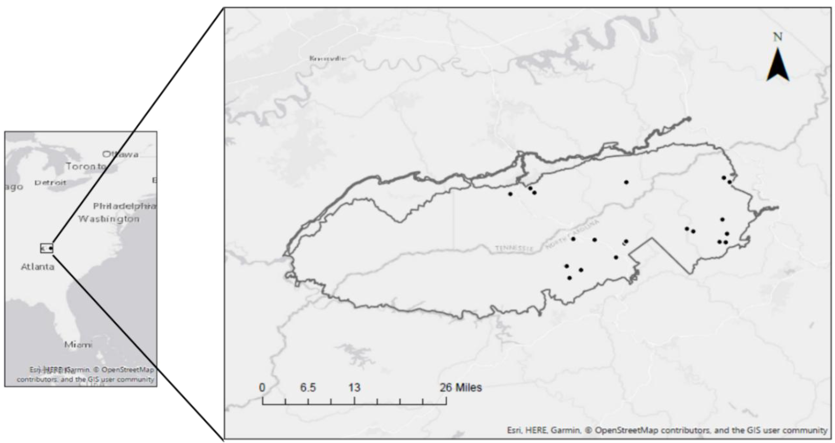
2.1. Study Area
2.2. Vegetation Sampling
2.3. Data Preparation
2.4. Statistical Analysis
2.4.1. Changes in Overstory Basal Area
2.4.2. Changes in Species Composition
2.4.3. Changes in Species Diversity
3. Results
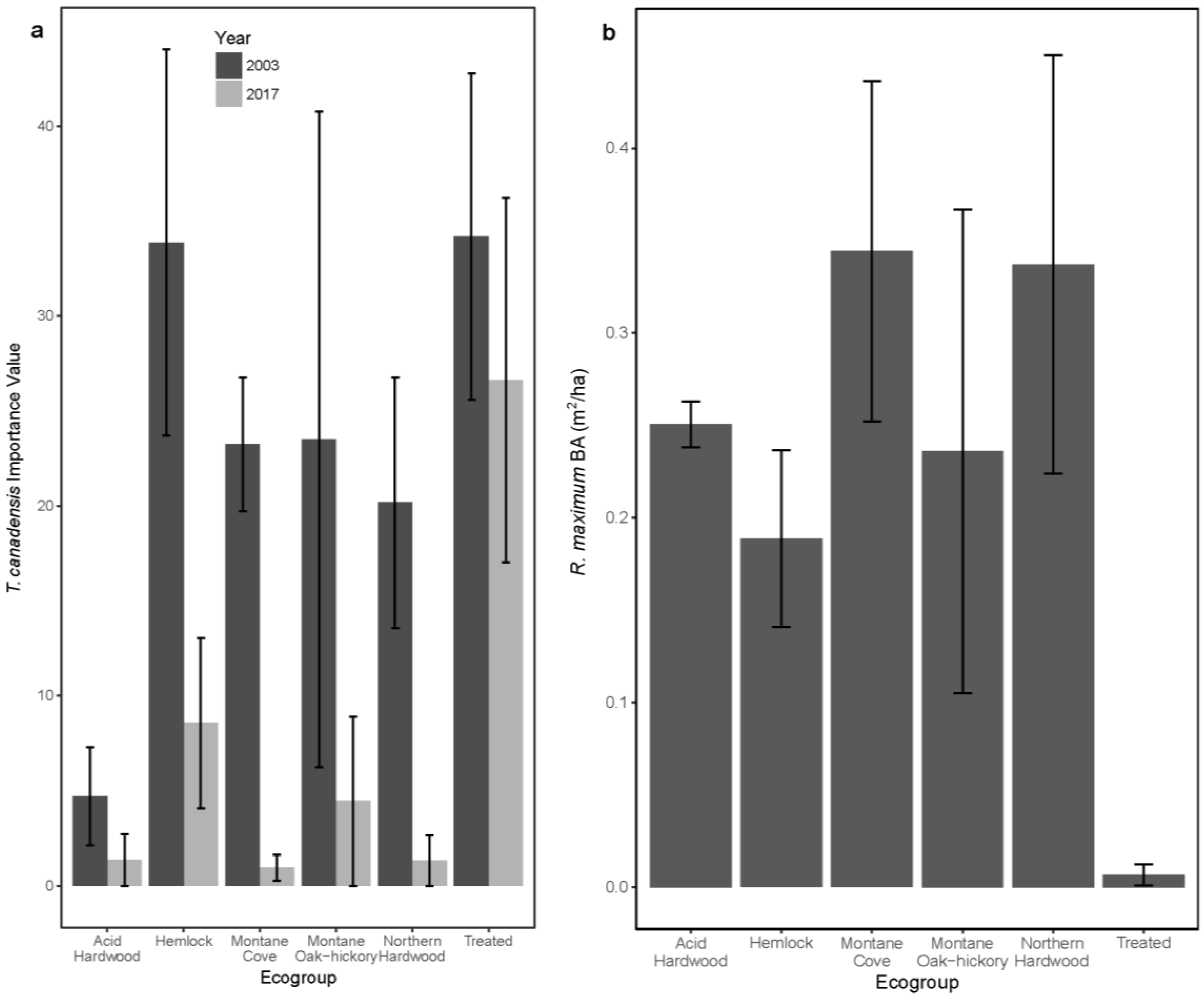
3.1. Overstory Basal Area and Species Importance
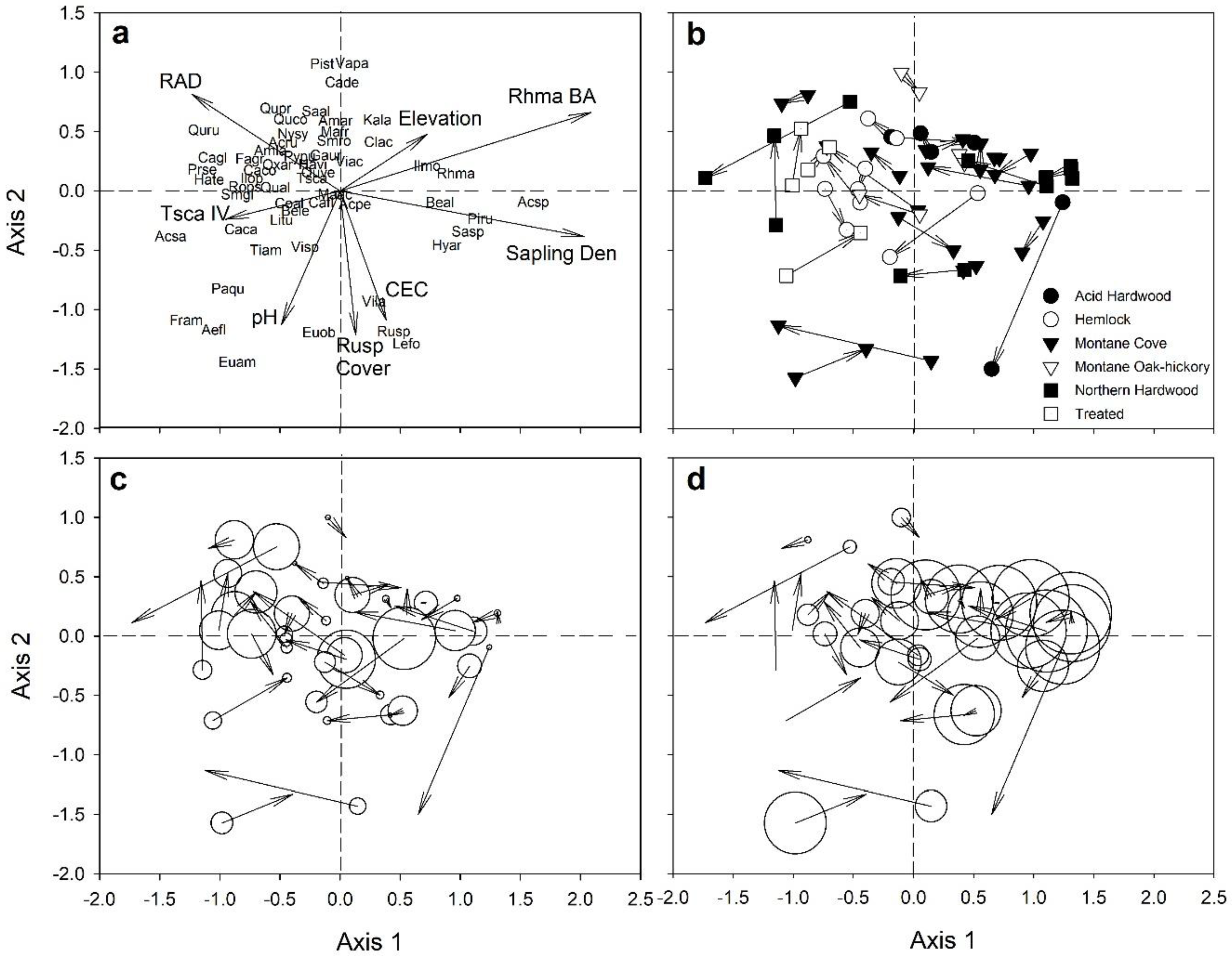
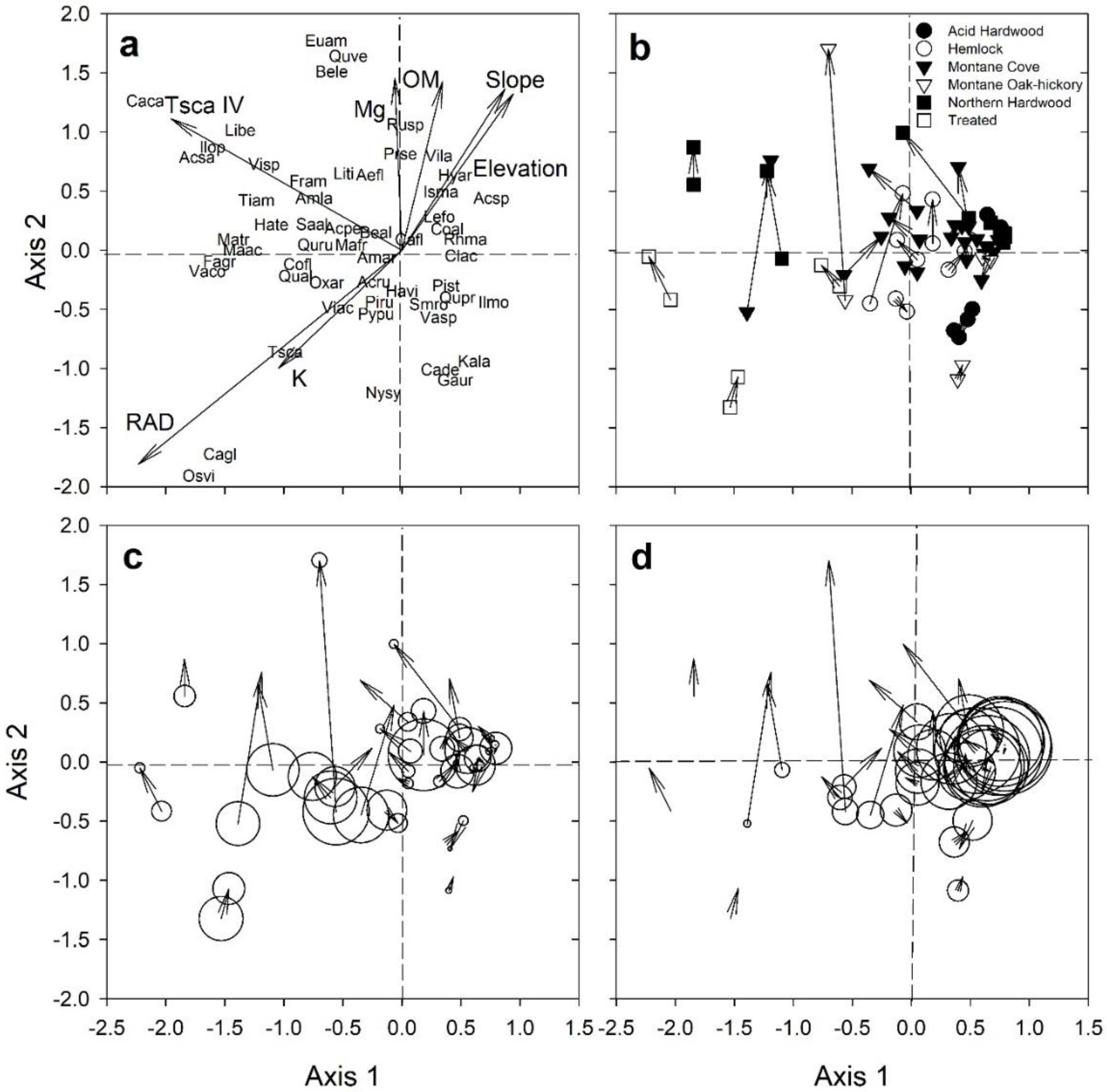
3.2. Seedling Species Composition
3.3. Sapling Species Composition
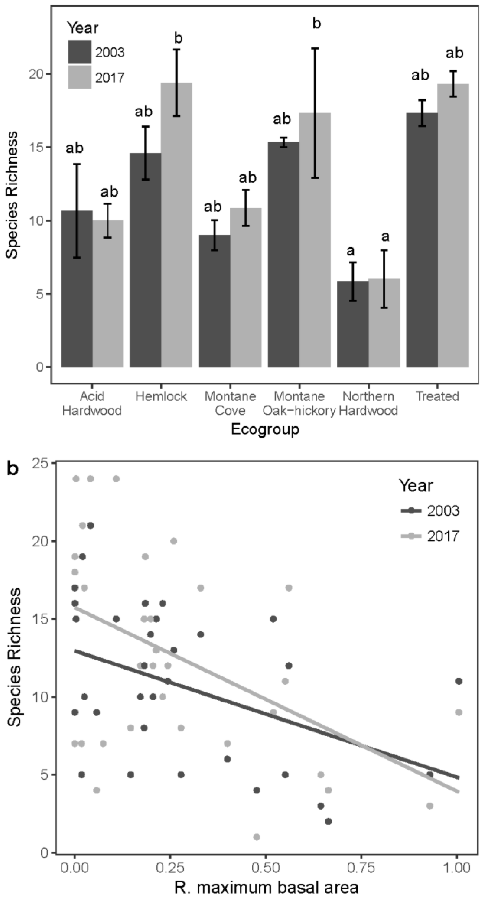
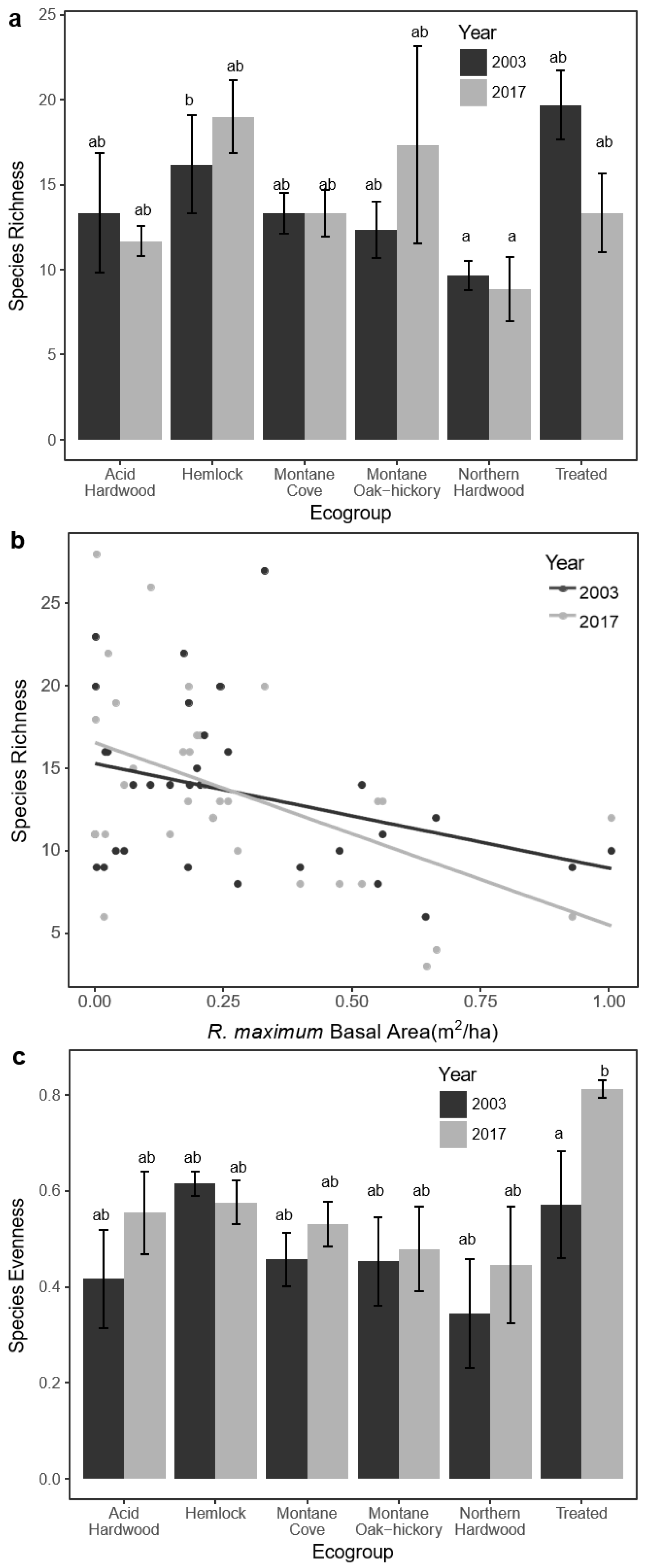
3.4. Seedling Species Diversity
3.5. Sapling Species Diversity
4. Discussion
Author Contributions
Funding
Acknowledgments
Conflicts of Interest
References
- McCullough, D.G.; Work, T.T.; Cavey, J.F.; Liebhold, A.M.; Marshall, D. Interceptions of nonindigenous plant pests at US ports of entry and border crossings over a 17-year period. Biol. Invasions 2006, 8, 611–630. [Google Scholar] [CrossRef]
- Westphal, M.I.; Browne, M.; MacKinnon, K.; Noble, I. The link between international trade and the global distribution of invasive alien species. Biol. Invasions 2008, 10, 391–398. [Google Scholar] [CrossRef]
- Work, T.T.; McCullough, D.G.; Cavey, J.F.; Komsa, R. Arrival rate of nonindigenous insect species into the United States through foreign trade. Biol. Invasions 2005, 7, 323–332. [Google Scholar] [CrossRef]
- Sala, O.E.; Chapin, F.S., III; Armesto, J.J.; Berlow, E.; Bloomfield, J.; Dirzo, R.; Huber-Sanwald, E.; Huenneke, L.F.; Jackson, R.B.; Kinzig, A.; et al. Global biodiversity scenarios for the year 2100. Science 2000, 287, 1700–1774. [Google Scholar] [CrossRef]
- Ellison, A.M.; Bank, M.S.; Clinton, B.D.; Colburn, E.A.; Elliott, K.; Ford, C.R.; Foster, D.R.; Kloeppel, B.D.; Knoepp, J.D.; Lovett, G.M.; et al. Loss of foundation species: Consequences for the structure and dynamics of forested ecosystems. Front. Ecol. Environ. 2005, 3, 479–486. [Google Scholar] [CrossRef]
- Gandhi, K.J.K.; Herms, D.A. Direct and indirect effects of alien insect herbivores on ecological processes and interactions in forests of eastern North America. Biol. Invasions 2010, 12, 389–405. [Google Scholar] [CrossRef]
- Lovett, G.M.; Canham, C.D.; Arthur, M.A.; Weathers, K.C.; Fitzhugh, R.D. Forest ecosystem responses to exotic pests and pathogens in eastern North America. BioScience 2006, 56, 395–405. [Google Scholar] [CrossRef]
- Aukema, J.E.; McCullough, D.G.; Von Holle, B.; Liebhold, A.M.; Britton, K.; Frankel, S.J. Historical accumulation of nonindigenous forest pests in the continental United States. BioScience 2010, 60, 886–897. [Google Scholar] [CrossRef]
- Kenis, M.; Auger-Rozenburg, M.; Roques, A.; Timms, L.; Péré, C.; Cock, M.J.W.; Settele, J.; Augustin, S.; Lopez-Vaamonde, C. Ecological effects of invasion alien insects. Biol. Invasions 2009, 11, 21–45. [Google Scholar] [CrossRef]
- McCormick, J.F.; Platt, R.B. Recovery of an Appalachian forest following the chestnut blight or Catherine Keever-You were right! Am. Midl. Nat. 1980, 104, 264–273. [Google Scholar] [CrossRef]
- Woods, F.W.; Shanks, R.E. Natural replacement of chestnut by other species in the Great Smoky Mountains National Park. Ecology 1959, 40, 349–361. [Google Scholar] [CrossRef]
- Keever, C. Present composition of some stands of the former oak-chestnut forest in the southern Blue Ridge Mountains. Ecology 1953, 34, 44–54. [Google Scholar] [CrossRef]
- McClure, M.S. Density-dependent feedback and population cycles in Adelges tsugae (Homoptera: Adelgidae) on Tsuga canadensis. Environ. Entomol. 1991, 20, 258–264. [Google Scholar] [CrossRef]
- Cheah, C.; Montgomery, M.E.; Salom, S.; Parker, B.L.; Costa, S.; Skinner, M. Biological Control of Hemlock Woolly Adelgid; Reardon, R., Onken, B., Eds.; FHTET, 2004-04; USDA Forest Service, Forest Health Technology Enterprise Team: Morgantown, WV, USA, 2004.
- Young, R.F.; Shields, K.S.; Berlyn, G.P. Hemlock woolly adelgid (Homoptera: Adelgidae): Stylet bundle insertion and feeding sites. Ann. Entom. Soc. Am. 1995, 88, 827–835. [Google Scholar] [CrossRef]
- Eschtruth, A.K.; Evans, R.A.; Battles, J.J. Patterns and predictors of survival in Tsuga canadensis populations infested by the exotic pest Adelges tsugae: 20 years of monitoring. For. Ecol. Manag. 2013, 305, 195–203. [Google Scholar] [CrossRef]
- Godman, R.M.; Lancaster, K. Tsuga canadensis. In Silvics of North America: Conifers; Burns, R.M., Honkala, B.H., Eds.; USDA Forest Service, Handbook; USDA Forest Service: Washington, DC, USA, 1990; Volume 1, pp. 604–612. [Google Scholar]
- Holzmueller, E.J.; Jose, S.; Jenkins, M.A. The relationship between fire history and an exotic fungal disease in a deciduous forest. Oecologia 2008, 155, 347–356. [Google Scholar] [CrossRef] [PubMed]
- Van Lear, D.H.; Vandermast, D.B.; Rivers, C.T.; Baker, T.T.; Hedman, C.W.; Clinton, D.B.; Waldrop, T.A. American Chestnut, Rhododendron, and the Future of Appalachian Cove Forests; Outcalt, K.W., Ed.; USDA Forest Service, Southern Research Station: Ashville, NC, USA, 2002; pp. 214–220.
- Toenies, M.J.; Miller, D.A.; Marshall, M.R.; Stauffer, G.E. Shifts in vegetation and avian community structure following the decline of a foundational forest species, the eastern hemlock. Condor Ornithol. Appl. 2018, 120, 489–506. [Google Scholar] [CrossRef]
- Eschtruth, A.K.; Cleavitt, N.L.; Battles, J.J.; Evans, R.A.; Fahey, T.J. Vegetation dynamics in declining eastern hemlock stands: 9 years of forest response to hemlock woolly adelgid infestation. Can. J. For. Res. 2006, 36, 1435–1450. [Google Scholar] [CrossRef]
- Foster, D.R.; Zebryk, T.M. Long-term vegetation dynamics and disturbance history of a Tsuga-dominated forest in New England. Ecology 1993, 74, 982–998. [Google Scholar] [CrossRef]
- Orwig, D.A.; Foster, D.R. Forest response to the introduced hemlock woolly adelgid in southern New England, USA. J. Torrey Bot. Soc. 1998, 125, 60–73. [Google Scholar] [CrossRef]
- Small, M.J.; Small, C.J.; Dreyer, G.D. Changes in a hemlock-dominated forest following woolly adelgid infestation in southern New England. J. Torrey Bot. Soc. 2005, 132, 458–470. [Google Scholar] [CrossRef]
- Orwig, D.A.; Plotkin, A.A.B.; Davidson, E.A.; Lux, H.; Savage, K.E.; Ellison, A.M. Foundation species loss affects vegetation structure more than ecosystem function in a northeastern USA forest. PeerJ 2013, 1, 1–29. [Google Scholar] [CrossRef] [PubMed]
- Johnson, K.; Remaley, T.; Taylor, G. Managing Hemlock Woolly Adelgid at Great Smoky Mountains National Park: Situation and Response; Onken, B., Reardon, R., Eds.; FHTET-2008-01; USDA Forest Service, Forest Health Technology Enterprise Team: Morgantown, WV, USA, 2008; pp. 62–69.
- Krapfl, K.J.; Holzmueller, E.J.; Jenkins, M.A. Early impacts of hemlock woolly adelgid in Tsuga canadensis forest communities of the southern Appalachian Mountains. J. Torrey Bot. Soc. 2011, 138, 93–106. [Google Scholar] [CrossRef]
- Spaulding, H.L.; Rieske, L.K. The aftermath of an invasion: Structure and composition of central Appalachian hemlock forests following establishment of the hemlock woolly adelgid, Adelges tsugae. Biol. Invasions 2010, 12, 3135–3143. [Google Scholar] [CrossRef]
- Krapfl, K.J.; Holzmueller, E.J.; Jenkins, M.A. Understory composition of five Tsuga canadensis associated forest communities in Great Smoky Mountains National Park. Nat. Areas J. 2012, 32, 260–269. [Google Scholar] [CrossRef]
- Ford, C.R.; Elliot, K.J.; Clinton, B.D.; Kloeppel, B.D.; Vose, J.M. Forest dynamics following eastern hemlock mortality in the southern Appalachians. Oikos 2012, 121, 523–536. [Google Scholar] [CrossRef]
- Elliot, K.J.; Vose, J.M. Age and distribution of an evergreen clonal shrub in Coweeta Basin: Rhododendron maximum L. J. Torrey Bot. Soc. 2012, 139, 149–166. [Google Scholar] [CrossRef]
- Jenkins, M.A. Vegetation communities of Great Smoky Mountains National Park. Southeast. Nat. 2007, 6, 35–56. [Google Scholar] [CrossRef]
- Southworth, S.; Schultz, A.; Denenny, D. Generalized Geologic Map of Bedrock Lithologies and Surficial Deposits in the Great Smoky Mountains National Park Region, Tennessee and North Carolina; Open-File Report 2004-1410, Version 1.0; U.S. Geological Survey: Reston, VA, USA, 2005.
- Whittaker, R.H. Vegetation of the Great Smoky Mountains. Ecol. Monogr. 1956, 26, 1–80. [Google Scholar] [CrossRef]
- White, R.D.; Patterson, K.D.; Weakley, A.; Ulrey, C.J.; Drake, J. Vegetation Classification of Great Smoky Mountains National Park; Report Submitted to BRDNPS Vegetation Mapping Program; NatureServe: Durham, NC, USA, 2003. [Google Scholar]
- Johnson, K.; Taylor, G.; Remaley, T. Managing hemlock woolly adelgid and balsam woolly adelgid at Great Smoky Mountains National Park. In Proceedings of the Third Symposium on Hemlock Woolly Adelgid in the Eastern United States, Asheville, NC, USA, 1–3 February 2005. [Google Scholar]
- Abella, S.R. Impacts and management of hemlock woolly adelgid in national parks of the eastern United States. Southeast. Nat. 2014, 13, 16–45. [Google Scholar]
- Webster, J. Management of hemlock woolly adelgid in Great Smoky Mountains National Park. In Proceedings of the Fifth Symposium on Hemlock Woolly Adelgid in the Eastern United States, Asheville, NC, USA, 17–19 August 2010. [Google Scholar]
- Jenkins, M.A. Great Smoky Mountains National Park: Vegetation Monitoring Protocol; National Park Service, Inventory and Monitoring Program, Great Smoky Mountains National Park: Gatlinburg, TN, USA, 2008. [Google Scholar]
- Mehlich, A. Mehlich 3 soil test extractant: A modification of Mehlich 2 extractant. Commun. Soil Sci. Plant. Anal. 1984, 15, 1409–1416. [Google Scholar] [CrossRef]
- McCune, B.; Grace, J.B. Analysis of Ecological Communities, 3rd ed.; MjM Software Design: Glaneden Beach, OR, USA, 2002. [Google Scholar]
- R Development Core Team. R: A Language and Environment for Statistical Computing; R Foundation for Statistical Computing: Vienna, Austria, 2016. [Google Scholar]
- McCune, B.; Keon, D. Equations for potential annual direct incident radiation and heat load. J. Veg. Sci. 2002, 13, 603–606. [Google Scholar] [CrossRef]
- Bates, D.; Maechler, M.; Bolker, B.; Walker, S. Fitting linear mixed-effects models using lme4. J. Stat. Soft. 2015, 67, 1–48. [Google Scholar] [CrossRef]
- Kuznetsova, A.; Brockhoff, P.B.; Christensen, R.H.B. LmerTest package: Tests in linear mixed effects models. J. Stat. Soft. 2017, 82, 1–26. [Google Scholar] [CrossRef]
- Laird, N.M.; Ware, J.H. Random-effects models for longitudinal data. Biometrics 1982, 38, 963–974. [Google Scholar] [CrossRef] [PubMed]
- Oksanen, J.; Blanchet, F.G.; Friendly, M.; Kindt, R.; Legendre, P.; Mcglinn, D.; Minchin, P.R.; O’Hara, R.B.; Simpson, G.L.; Solymos, P.; et al. Vegan: Community Ecology Package. R Package Version 2.4-5. 2017. Available online: https://CRAN.R-project.org/package=vegan (accessed on 3 October 2017).
- Leth, R.V. Least-squares means: The R package lsmeans. J. Stat. Soft. 2016, 69, 1–33. [Google Scholar]
- Jenkins, J.C.; Aber, J.D.; Canham, C.D. Hemlock woolly adelgid impacts on community structure and N cycling rates in eastern hemlock forests. Can. J. Res. 1999, 29, 630–645. [Google Scholar] [CrossRef]
- Lustenhouwer, M.N.; Nicoll, L.; Ellison, A.M. Microclimate effects of the loss of a foundation species from New England forests. Ecosphere 2012, 3, 1–16. [Google Scholar] [CrossRef]
- Orwig, D.A.; Cobb, R.C.; D’Amato, A.W.; Kizlinski, M.L.; Foster, D.R. Multi-year ecosystem response to hemlock woolly adelgid infestation in southern New England forests. Can. J. Res. 2008, 38, 834–843. [Google Scholar] [CrossRef]
- Vose, J.M.; Wear, D.N.; Mayfield, A.E., III; Nelson, C.D. Hemlock woolly adelgid in the southern Appalachians: Control strategies, ecological impacts, and potential management responses. For. Ecol. Manag. 2013, 291, 209–219. [Google Scholar] [CrossRef]
- Cofer, T.M.; Elliott, K.J.; Bush, J.K.; Miniat, C.F. Rhododendron maximum impacts seed bank composition and richness following Tsuga canadensis loss in riparian forests. Ecosphere 2018, 9, e02204. [Google Scholar] [CrossRef]
- Nilsen, E.T.; Clinton, B.D.; Lei, T.T.; Miller, O.K.; Semones, S.W.; Walker, J.F. Rhododendron maximum L. (Ericaceae) reduce the availability of resources above and belowground for canopy tree seedlings? Am. Midl. Nat. 2001, 145, 325–343. [Google Scholar] [CrossRef]
- Phillips, D.L.; Murdy, W.H. Effects of rhododendron (Rhododendron maximum L.) on regeneration of southern Appalachian hardwoods. For. Sci. 1985, 31, 226–233. [Google Scholar]
- Roberts, S.W.; Tankersley, R., Jr.; Orvis, K.H. Assessing the potential impacts to riparian ecosystems resulting from hemlock mortality in Great Smoky Mountains National Park. Environ. Manag. 2009, 44, 335–345. [Google Scholar] [CrossRef]
- Wurzburger, N.; Hendrick, R.L. Rhododendron thickets alter N cycling and soil extracellular enzyme activities in southern Appalachian hardwood forests. Pedobiologia 2007, 50, 563–576. [Google Scholar] [CrossRef]
- McGee, C.E.; Smith, R.C. Undisturbed rhododendron thickets are not spreading. J. For. 1967, 65, 334–335. [Google Scholar]
- Plocher, A.E.; Carvell, K.L. Population dynamics of rosebay rhododendron thickets in the southern Appalachians. Bull. Torrey Bot. Club 1987, 114, 121–126. [Google Scholar] [CrossRef]
- Goebel, P.C.; Hix, D.M. Changes in the composition and structure of mixed-oak, second-growth forest ecosystems during the understory reinitiation stage of stand development. Ecoscience 1997, 4, 327–339. [Google Scholar] [CrossRef]
- Jenkins, M.A.; Parker, G.R. Composition and diversity of woody vegetation in silvicultural openings of southern Indiana forests. For. Ecol. Manag. 1998, 109, 57–74. [Google Scholar] [CrossRef]
- Pallardy, S.G. Vegetation analysis, environmental relationships, and potential successional trends in Missouri Forest Ecosystem Project. In Proceedings of the 10th Central Hardwood Forest Conference, Morgantown, WV, USA, 5–8 March 1995. [Google Scholar]
- Elliott, K.J.; Knoepp, J.D. The effects of three regeneration harvest methods on plant diversity and soil characteristics in the southern Appalachians. For. Ecol. Manag. 2005, 211, 296–317. [Google Scholar] [CrossRef]
- Case, B.S.; Buckley, H.L.; Barker-Plotkin, A.A.; Orwig, D.A.; Ellison, A.M. When a foundation crumbles: Forecasting forest dynamics following the decline of the foundation species Tsuga canadensis. Ecosphere 2017, 8, e01893. [Google Scholar] [CrossRef]
- Boettcher, S.E.; Kalisz, P.J. Single-tree influence on soil properties in the mountains of eastern Kentucky. Ecology 1990, 71, 1365–1372. [Google Scholar] [CrossRef]
- Finzi, A.C.; van Breemen, N.; Canham, C.D. Canopy tree-soil interactions within temperate forests: Species effects on soil carbon and nitrogen. Ecol. Appl. 1998, 8, 440–446. [Google Scholar]
- Finzi, A.C.; Canham, C.D.; van Breemen, N. Canopy tree-soil interactions within temperate forests: Species effects on pH and cations. Ecol. Appl. 1998, 8, 447–454. [Google Scholar]
- Brantley, S.; Ford, C.R.; Vose, J.M. Future species composition will affect forest water use after loss of eastern hemlock. Ecol. Appl. 2013, 23, 777–790. [Google Scholar] [CrossRef]
- Ford, C.R.; Vose, J.M. Tsuga canadensis (L.) Carr. mortality will impact hydrologic processes in southern Appalachian forest ecosystems. Ecol. Appl. 2007, 17, 1156–1167. [Google Scholar] [CrossRef]
- Knoepp, J.D.; Vose, J.M.; Clinton, B.D.; Hunter, M.D. Hemlock infestation and mortality: Impacts on nutrient pools and cycling in Appalachian forests. Soil Sci. Soc. Am. J. 2011, 75, 1935–1945. [Google Scholar] [CrossRef]
- Yorks, T.E.; Leopold, D.J.; Raynal, D.J. Effects of Tsuga canadensis mortality on soil water chemistry and understory vegetation: Possible consequences of an invasive herbivore. Can. J. For. Res. 2003, 33, 1525–1537. [Google Scholar] [CrossRef]


| Year | Acid Hardwood (n = 3) | Hemlock (n = 5) | Montane Cove (n = 13) | Montane Oak-Hickory (n = 3) | Northern Hardwood (n = 6) | Total (n = 30) | Treated (n = 3) |
|---|---|---|---|---|---|---|---|
| 2003 | 31.3 ± 4.6 | 33.7± 1.5 | 31.4 ± 2.2 | 35.4 ± 6.0 | 31.6 ± 5.8 | 32.2 ± 1.5 | 31.8 ± 2.8 |
| 2017 | 31.0 ± 2.1 | 28.8 ± 5.0 | 28.2 ± 2.4 | 27.0 ± 4.8 | 24.9 ± 3.6 | 27.8 ± 1.5 | 34.6 ± 1.7 |
| Species | Acid Hardwood (n = 3) | Hemlock (n = 5) | Montane Cove (n = 13) | Montane Oak-Hickory (n = 3) | Northern Hardwood (n = 6) | Treated (n = 3) | ||||||
|---|---|---|---|---|---|---|---|---|---|---|---|---|
| 2003 | 2017 | 2003 | 2017 | 2003 | 2017 | 2003 | 2017 | 2003 | 2017 | 2003 | 2017 | |
| Acer pensylvanicum | 2.5 ± 1.3 | 3.2 ± 1.8 | 0.6 ± 0.6 | 2.0 ± 1.3 | 2.4 ± 1.7 | 2.0 ± 1.7 | 0.6 ± 0.6 | 0 | 2.9 ± 2.3 | 4.5 ± 3.9 | 0 | 0 |
| Acer rubrum | 11.6 ± 6.4 | 11.4 ± 7.1 | 13.0 ± 5.6 | 13.6 ± 5.5 | 7.6 ± 2.2 | 9.8 ± 3.1 | 21.8 ± 9.0 | 26.8 ± 8.7 | 0.3 ± 0.3 | 1.7 ± 1.1 | 5.8 ± 1.8 | 7.7 ± 1.5 |
| Acer saccharum | 0 | 0 | 0 | 2.2 ± 2.2 | 0 | 1.0 ± 0.4 | 0.6 ± 0.6 | 1.3 ± 1.3 | 6.2 ± 3.4 | 8.6 ± 4.1 | 2.2 ± 1.6 | 2.3 ± 2.3 |
| Amelanchier laevis | 7.4 ± 6.0 | 6.8 ± 5.6 | 0 | 0 | 0.6 ± 0.4 | 0.1 ± 0.1 | 0.6 ± 0.6 | 0.7 ± 0.7 | 0.6 ± 0.6 | 0.7 ± 0.7 | 0 | 0 |
| Betula alleghaniensis | 13.0 ± 9.7 | 14.0 ± 10.6 | 5.4 ± 3.4 | 4.0 ± 2.5 | 9.6 ± 3.5 | 14.3 ± 5.1 | 1.3 ± 1.3 | 4.4 ± 4.4 | 18.4 ± 7.9 | 22.5 ± 8.5 | 0.4 ± 0.4 | 0.5 ± 0.5 |
| Betula lenta | 5.0 ± 0.2 | 2.6 ± 1.1 | 10.3 ± 2.7 | 20.7 ± 6.0 | 12.4 ± 5.0 | 15.6 ± 5.4 | 5.2 ± 3.5 | 6.4 ± 3.9 | 3.5 ± 1.8 | 4.7 ± 2.7 | 3.8 ± 1.3 | 5.6 ± 2.2 |
| Fagus grandifolia | 5.3 ± 4.3 | 8.3 ± 6.8 | 0.3 ± 0.3 | 0.4 ± 0.4 | 5.5 ± 2.3 | 4.8 ± 2.2 | 0 | 0 | 12.5 ± 4.4 | 13.4 ± 3.2 | 0.8 ± 0.8 | 1.6 ± 0.9 |
| Halesia tetraptera | 1.8 ± 1.5 | 0 | 3.5 ± 1.1 | 5.7 ± 3.0 | 5.0 ± 1.3 | 6.2 ± 1.6 | 0.6 ± 0.6 | 0.6 ± 0.6 | 7.3 ± 3.4 | 11.3 ± 5.1 | 0.4 ± 0.4 | 0.5 ± 0.5 |
| Liriodendron tulipifera | 0 | 0 | 4.4 ± 1.4 | 8.2 ± 2.4 | 1.9 ± 1.0 | 2.8 ± 1.5 | 2.0 ± 2.0 | 4.4 ± 4.4 | 0 | 0 | 15.0 ± 5.9 | 18.9 ± 8.5 |
| Magnolia fraseri | 5.4 ± 4.4 | 8.2 ± 6.7 | 1.6 ± 1.0 | 2.2 ± 1.6 | 2.1 ± 1.1 | 4.5 ± 1.8 | 1.9 ± 1.9 | 1.3 ± 1.3 | 1.6 ± 0.8 | 3.0 ± 1.3 | 0 | 0 |
| Nyssa sylvatica | 3.6 ± 2.9 | 2.5 ± 2.1 | 0.3 ± 0.3 | 0.3 ± 0.3 | 1.2 ± 0.6 | 1.2 ± 0.8 | 1.7 ± 1.7 | 1.7 ± 1.7 | 0.3± 0.3 | 0.6 ± 0.6 | 1.3 ± 1.3 | 2.1 ± 2.1 |
| Oxydendrum arboreum | 6.3 ± 5.1 | 5.0 ± 4.1 | 4.4 ± 3.3 | 4.5 ± 3.2 | 4.5 ± 2.0 | 6.3 ± 3.0 | 9.0 ± 2.5 | 13.1 ± 0.6 | 0 | 0 | 5.4 ± 3.7 | 4.7 ± 3.3 |
| Picea rubens | 16.0 ± 8.9 | 12.4 ± 5.9 | 0 | 0 | 2.9 ± 2.8 | 3.8 ± 3.6 | 0 | 0 | 0 | 0 | 0 | 0 |
| Pinus strobus | 0 | 0 | 4.6 ± 4.6 | 4.4 ± 4.4 | 0.8 ± 0.8 | 0.8 ± 0.8 | 0 | 0 | 0 | 0 | 0 | 0 |
| Quercus prinus | 6.1 ± 4.1 | 4.5 ± 2.4 | 1.3 ± 0.9 | 1.9 ± 1.6 | 2.6 ± 1.4 | 2.7 ± 1.5 | 12.8 ± 9.6 | 11.8 ± 10.1 | 0 | 0 | 0.4 ± 0.4 | 0.5 ± 0.5 |
| Quercus rubra | 3.7 ± 3.0 | 3.4± 2.8 | 2.2 ± 1.2 | 1.7 ± 0.8 | 2.3 ± 0.9 | 2.7 ± 1.4 | 2.5 ± 2.5 | 2.0 ± 2.0 | 0.3 ± 0.3 | 0.6 ± 0.6 | 0.8 ± 0.4 | 1.0 ± 0.5 |
| Rhododendron maximum | 1.6 ± 0.7 | 1.3 ± 0.5 | 1.2 ± 0.6 | 3.6 ± 2.0 | 4.6 ± 2.4 | 6.6 ± 2.2 | 5.1 ± 5.1 | 5.2 ± 5.2 | 3.4 ± 1.4 | 8.1 ± 3.6 | 0 | 0 |
| Tilia americana | 0 | 0 | 5.9 ± 5.9 | 5.9 ± 4.9 | 6.0 ± 3.1 | 7.5 ± 3.6 | 0 | 0 | 15.6 ± 9.4 | 12.3 ± 5.5 | 2.3 ± 0.8 | 3.1 ± 1.6 |
| Tsuga canadensis | 4.7 ± 2.1 | 1.4 ± 1.1 | 33.9 ± 11.2 | 8.6 ± 4.5 | 23.2 ± 3.5 | 0.9 ± 0.7 | 23.5 ± 17.3 | 4.4 ± 4.4 | 20.2 ± 6.6 | 1.3 ± 1.3 | 34.2 ± 8.6 | 26.6 ± 9.6 |
| Environmental Variable | Seedling | Sapling | ||
|---|---|---|---|---|
| R2 | p | R2 | p | |
| RAD | 0.245 | 0.003 | 0.320 | 0.001 |
| CEC | 0.168 | 0.010 | 0.007 | 0.819 |
| pH | 0.160 | 0.014 | 0.036 | 0.363 |
| OM | 0.033 | 0.555 | 0.083 | 0.081 |
| P (ppm) | 0.182 | 0.008 | 0.025 | 0.455 |
| Ca (ppm) | 0.372 | 0.001 | 0.059 | 0.156 |
| K (ppm) | 0.043 | 0.471 | 0.081 | 0.086 |
| Mg (ppm) | 0.395 | 0.001 | 0.082 | 0.087 |
| Elevation | 0.185 | 0.006 | 0.103 | 0.048 |
| Slope (%) | 0.075 | 0.193 | 0.102 | 0.046 |
| Pre-HWA T. canadensis IV | 0.230 | 0.003 | 0.196 | 0.003 |
| R. maximum basal area | 0.524 | 0.001 | -- | -- |
| Sapling density | 0.468 | 0.001 | -- | -- |
| Rubus spp. percent cover | 0.178 | 0.004 | -- | -- |
| Ecogroup | 0.125 | 0.074 | 0.303 | 0.001 |
| Acid Hardwood (n = 3) | Hemlock (n = 5) | Montane Cove (n = 12) | Montane Oak- Hickory (n = 3) | Northern Hardwood (n = 6) | Treated (n = 3) | |||||||
|---|---|---|---|---|---|---|---|---|---|---|---|---|
| 2003 | 2017 | 2003 | 2017 | 2003 | 2017 | 2003 | 2017 | 2003 | 2017 | 2003 | 2017 | |
| Seedlings | ||||||||||||
| S | 10.67 ± 3.18 | 10.00 ± 1.15 | 14.60 ± 1.81 | 19.40 ± 2.27 | 9.00 ± 1.02 | 10.85 ± 1.22 | 15.33 ± 0.33 | 17.33 ± 4.41 | 5.83 ± 1.30 | 6.00 ± 2.00 | 17.33 ± 0.88 | 19.33 ± 0.88 |
| E | 0.73 ± 0.10 | 0.72 ± 0.063 | 0.67 ± 0.035 | 0.76 ± 0.046 | 0.63 ± 0.047 | 0.64 ± 0.041 | 0.75 ± 0.029 | 0.75 ± 0.034 | 0.57 ± 0.073 | 0.70 ± 0.12 | 0.83 ± 0.040 | 0.64 ± 0.039 |
| H′ | 1.72 ± 0.43 | 1.67 ± 0.22 | 1.80 ± 0.16 | 2.25 ± 0.18 | 1.40 ± 0.17 | 1.47 ± 0.13 | 2.06 ± 0.089 | 2.09 ± 0.30 | 1.00 ± 0.25 | 1.10 ± 0.35 | 2.37 ± 0.079 | 1.90 ± 0.088 |
| Saplings | ||||||||||||
| S | 13.33 ± 3.53 | 11.67 ± 0.88 | 16.20 ± 2.87 | 19.0 ± 2.12 | 13.31 ± 1.22 | 13.31 ± 1.36 | 12.33 ± 1.67 | 17.33 ± 5.81 | 9.67 ± 0.084 | 8.83 ± 1.89 | 19.67 ± 2.03 | 13.33 ± 2.33 |
| E | 0.42 ± 0.10 | 0.55 ± 0.087 | 0.62 ± 0.025 | 0.58 ± 0.046 | 0.46 ± 0.055 | 0.53 ± 0.047 | 0.46 ± 0.092 | 0.48 ± 0.088 | 0.34 ± 0.11 | 0.45 ± 0.12 | 0.57 ± 0.11 | 0.81 ± 0.017 |
| H′ | 1.10 ± 0.34 | 1.37 ± 0.25 | 1.67 ± 0.080 | 1.70 ± 0.19 | 1.19 ± 0.16 | 1.37 ± 0.15 | 1.10 ± 0.16 | 1.37 ± 0.42 | 0.79 ± 0.27 | 1.05 ± 0.33 | 1.67 ± 0.29 | 2.08 ± 0.10 |
| Shannon-Weaver Diversity | Species Richness | Species Evenness | ||||||||
|---|---|---|---|---|---|---|---|---|---|---|
| df | MS | F | p | MS | F | p | MS | F | p | |
| Seedlings | ||||||||||
| Year | 1 | 0.013 | 0.08 | 0.78 | 0.01 | 0.05 | 0.82 | 0.005 | 0.002 | 0.97 |
| Ecogroup | 5 | 0.44 | 2.66 | 0.045 | 0.75 | 4.63 | 0.005 | 0.20 | 0.75 | 0.59 |
| R. maximum BA | 1 | 0.69 | 4.15 | 0.052 | 0.01 | 0.08 | 0.78 | -- | -- | -- |
| Year × Ecogroup | 5 | 0.41 | 2.51 | 0.055 | 0.14 | 0.85 | 0.53 | 0.86 | 3.20 | 0.022 |
| Year × R. maximum | ||||||||||
| BA | 1 | -- | -- | -- | 0.06 | 0.34 | 0.56 | -- | -- | -- |
| Ecogroup × R. maximum | ||||||||||
| BA | 5 | -- | -- | -- | 0.22 | 1.34 | 0.29 | -- | -- | -- |
| Year × | ||||||||||
| Ecogroup × | ||||||||||
| R. maximum BA | 5 | -- | -- | -- | 0.44 | 2.70 | 0.049 | -- | -- | -- |
| Saplings | ||||||||||
| Year | 1 | 1.92 | 12.99 | 0.001 | 0.028 | 0.11 | 0.74 | 2.52 | 22.75 | <0.001 |
| Ecogroup | 5 | 0.24 | 1.61 | 0.19 | 0.81 | 3.23 | 0.026 | 0.11 | 1.01 | 0.43 |
| R. maximum BA | 1 | 5.08 | 34.54 | <0.001 | 0.51 | 2.01 | 0.17 | 4.39 | 39.69 | <0.001 |
| Year × Ecogroup | 5 | 0.093 | 0.63 | 0.68 | 0.19 | 0.77 | 0.58 | 0.43 | 3.87 | 0.009 |
| Year × R. maximum | ||||||||||
| BA | 1 | -- | -- | -- | 0.015 | 0.058 | 0.81 | -- | -- | -- |
| Ecogroup × R. maximum | ||||||||||
| BA | 5 | -- | -- | -- | 0.24 | 0.95 | 0.47 | -- | -- | -- |
| Year × | ||||||||||
| Ecogroup × R. maximum | ||||||||||
| BA | 5 | -- | -- | -- | 1.73 | 6.86 | 0.0006 | -- | -- | -- |
© 2019 by the authors. Licensee MDPI, Basel, Switzerland. This article is an open access article distributed under the terms and conditions of the Creative Commons Attribution (CC BY) license (http://creativecommons.org/licenses/by/4.0/).
Share and Cite
Mulroy, M.L.; Holzmueller, E.J.; Jenkins, M.A. Woody Regeneration Response to Overstory Mortality Caused by the Hemlock Woolly Adelgid (Adelges tsugae) in the Southern Appalachian Mountains. Forests 2019, 10, 717. https://doi.org/10.3390/f10090717
Mulroy ML, Holzmueller EJ, Jenkins MA. Woody Regeneration Response to Overstory Mortality Caused by the Hemlock Woolly Adelgid (Adelges tsugae) in the Southern Appalachian Mountains. Forests. 2019; 10(9):717. https://doi.org/10.3390/f10090717
Chicago/Turabian StyleMulroy, Meghan L., Eric J. Holzmueller, and Michael A. Jenkins. 2019. "Woody Regeneration Response to Overstory Mortality Caused by the Hemlock Woolly Adelgid (Adelges tsugae) in the Southern Appalachian Mountains" Forests 10, no. 9: 717. https://doi.org/10.3390/f10090717
APA StyleMulroy, M. L., Holzmueller, E. J., & Jenkins, M. A. (2019). Woody Regeneration Response to Overstory Mortality Caused by the Hemlock Woolly Adelgid (Adelges tsugae) in the Southern Appalachian Mountains. Forests, 10(9), 717. https://doi.org/10.3390/f10090717