Evaluation of Stand Biomass Estimation Methods for Major Forest Types in the Eastern Da Xing’an Mountains, Northeast China

Abstract

Currently, forest biomass estimation methods at the regional scale have attracted the greatest attention from researchers, and the development of stand biomass models has become popular a trend. In this study, a total of 5074 measurements on 1053 permanent sample plots were obtained in the Eastern Da Xing’an Mountains, and three additive systems of stand biomass equations were developed. The first additive system (M-1) used stand variables as the predictors (i.e., stand basal area and average height), the second additive system (M-2) utilized stand volume as the sole predictor, and the third additive system (M-3) included both stand volume and biomass expansion and conversion factors (BCEFs) as the predictors. The coefficients of the three model systems were estimated with nonlinear seemingly unrelated regression (NSUR), while the heteroscedasticity of the model residuals was solved with the weight function. The jackknifing technique was used on the residuals, and several statistics were used to assess the prediction performance of each model. We comprehensively evaluated four stand biomass estimation methods (i.e., M-1, M-2, M-3 and a constant BCEF (M-4)). Here, we showed that the (1) three additive systems of stand biomass equations showed good model fitting and prediction performance, (2) M-3 significantly improved the model fitting and performance and provided the most accurate predictions for most stand biomass components, and (3) the ranking of the four stand biomass estimation methods followed the order of M-3 > M-2 > M-4 > M-1. Our results demonstrated these additive stand biomass models could be used to estimate the stand aboveground and belowground biomass for the major forest types in the Eastern Da Xing’an Mountains, although the most appropriate method depends on the available data and forest type.

1. Introduction

Among the studies on global climate change and the carbon cycle, research on the quantity, distribution, and dynamics of forest carbon stocks is popular and remains a high priority for predicting the growth and yield of forests [1,2,3]. Since the carbon concentrations in a tree or stand components are relatively constant (approximately 50%), most studies focus on forest biomass estimations rather than carbon storage estimations. Thus, the calculation of accurate forest biomass estimations has become one of the most crucial steps for successfully implementing the Reducing Emissions from Deforestation and Forest Degradation (REDD+) project as well as for the conservation and enhancement of forest carbon stocks and the sustainable management of forests. These initiatives provide a framework that benefits developing countries by rewarding them financially to reduce carbon emissions [4,5]. To date, different countries have used various methods for their national-scale carbon assessments, which differ in the degree of accuracy and the amount of field inventory [6,7,8,9,10].

Forest stand biomass can be estimated at either the tree or stand level. At the tree level, the most commonly used method is the allometric equation, which estimates tree biomass using simple tree variables, such as the tree diameter at breast height (D) and/or tree height (H) [11,12,13,14]. Tree allometric equations require inventories that have high cost and time requirements, although they yield high accuracies for estimating tree biomass. The sum of the biomasses of individual trees provides the biomass for a plot or stand. Alternatively, the stand biomass can be estimated using either stand biomass models or biomass expansion and conversion factors (BCEFs), which represent the ratio of the stand biomass to stand volume. Historically, most biomass studies in the literature have focused on tree biomass models, while efforts related to stand biomass models have been limited or lacking [6,7,9,10,15]. For the stand biomass estimations, some researchers believe that the use of stand biomass models can more easily estimate the stand biomass and prevent having to address complex error propagation procedures at different spatial scales [6,7].

In recent years, with the rapid accumulation of forest biomass data throughout the world, researchers have attempted to improve forest biomass estimations and proposed various stand biomass estimation methods [7,10,16,17,18]. Studies have shown that stand biomass is closely related to some easily measured stand variables, such as the quadratic mean diameter, average height, and basal area of the stand [7,8,19]. In addition, the total and individual components of stand biomass have a strong correlation with stand volume, which has been used as a predictor in stand biomass models [20,21,22]. Recent methodology guidelines from the IPCC [23] provided a set of species-specific default values for BCEFs. It is well known that using a constant BCEF to quantify stand biomass produces certain biases or errors because BCEFs vary depending on the growth conditions and stand development stage, such as the stand age, stand size and stand density [15,16,21]. Studies have noted that BCEFs are not constant, and linear models have been established between stand biomass and volume [20,24,25]. Other researchers constructed nonlinear models (e.g., hyperbolic functions, reciprocal equations, and power functions) to express the relationships between stand biomass and BCEFs [7,10,15,16,17,26]. Overall, using stand biomass models with stand volume as the sole predictor or expanding the stand volume with an available BCEF is a relatively simple method for estimating stand biomass [7]. However, few comparative evaluations have been performed for different stand biomass estimation methods in the literature, especially for predicting stand biomass across a large geographic region.

When more than one biomass component is found in the same sample plot, the stand biomass equation is used to fit the total and component biomass data simultaneously, which explains the inherent correlations among the biomasses of the stand components in the same sample plot [6,12,13]. Consequently, the sum of stand biomass predictions from the component biomass models and the total biomass model are the same. To achieve the additivity of stand biomass equations, various parameter estimation methods and model specifications are used in linear and nonlinear models [11,12,27,28,29]. Among these methods of parameter estimation, nonlinear seemingly unrelated regression (NSUR) and seemingly unrelated regression (SUR) are the most widely used. An advantage of SUR and NSUR is the low variance of the total stand biomass model because of their own predictor variables and weighting function account for heteroscedasticity, which makes SUR and NSUR popular methods for parameter estimation in nonlinear and linear stand biomass equations [11,12,13,14,30]. Although several researchers have proposed the inclusion of additivity, it has often been ignored in some stand biomass models [8,10].

Additionally, similar to tree biomass models, stand biomass models commonly show heteroscedastic model residuals. To overcome the heteroscedasticity of the stand biomass model residuals, logarithmic transformation or a weighted regression should be performed before the construction of each carbon model [12,13]. To acquire an ideal result from logarithmic regression, a correction is necessary after the antilog transformation, i.e., the predicted values are multiplied by a correction factor [31,32]. However, when determining the total and component equations of stand biomass, after applying the correction factor to the logarithmic equations of the additive system, realizing additivity is difficult [32]. Thus, the weighted regression successfully overcomes the heteroscedasticity of the total and component biomass model residuals in an additive system [12,13].

Asia is one of three primary locations of temperate mixed forests worldwide (i.e., northeastern North America, Europe, and eastern Asia), and they are mainly distributed in the forest regions of northeastern China. Chinese temperate forests are widely distributed in the Eastern Da Xing’an Mountains. These temperate forests play a crucial role in the Chinese national carbon budget and climatic system. Unfortunately, the forest resource inventory data in this region have not been fully utilized, and only limited stand biomass models are available. Thus, the objectives of this study were to (1) develop three alternative additive systems of stand biomass equations (i.e., stand biomass models using stand variables (M-1), stand biomass models using stand volume (M-2), and stand biomass models using both stand volume and BCEF (M-3)) for estimating the stand biomass of major forest types (including white birch forest, larch forest, poplar-birch forest, deciduous broadleaf mixed forest, coniferous and broadleaf mixed forest, and coniferous mixed forest) in the Eastern Da Xing’an Mountains, Northeast China, (2) use the jackknife method to validate the performance of those stand biomass models, and (3) evaluate the predictive ability of four alternative methods (i.e., M-1, M-2, M-3, and constant BCEF (M-4)) to estimate the total and component biomasses in each forest stand.

2. Materials and Methods

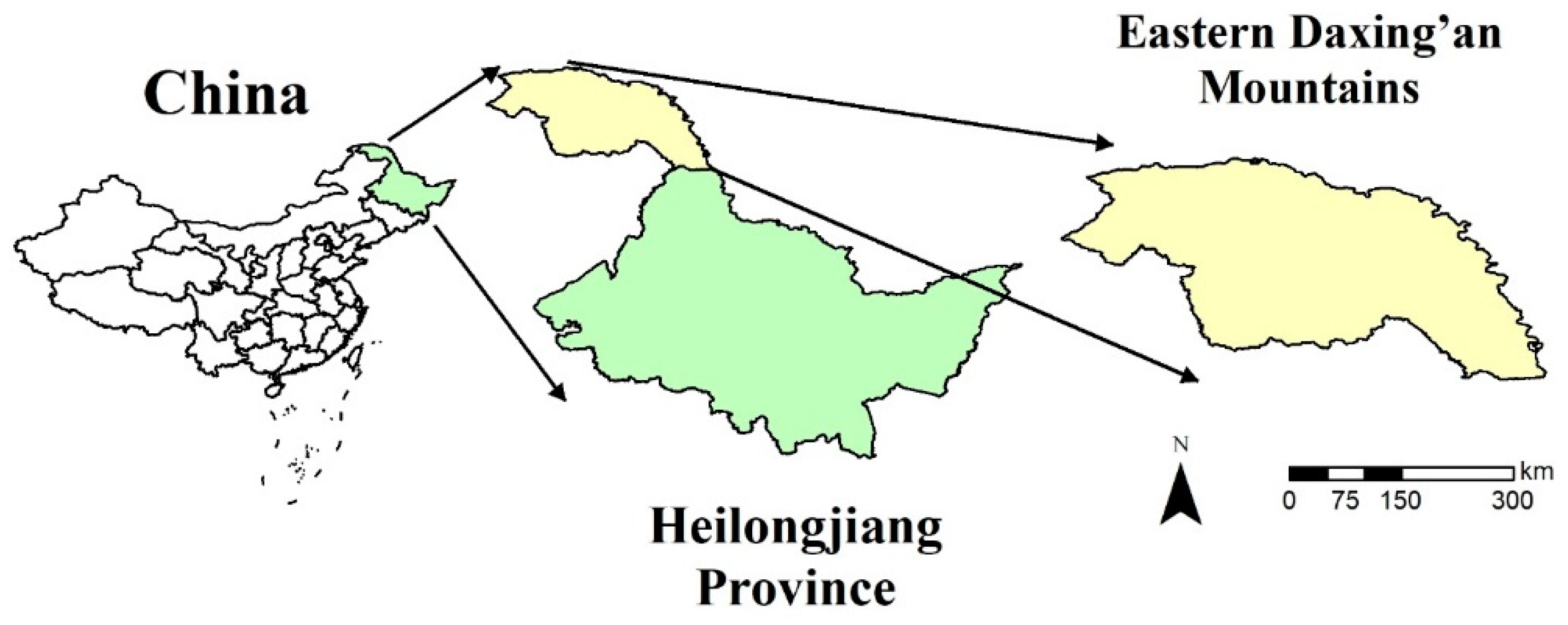
2.1. Study Area and Data

The Eastern Da Xing’an Mountains in Northeast China are defined as in our previous study [14], and they cover an area of 83,517 km² (Figure 1). The terrain, soil, and climate of the region were described in Dong et al. [14] and, thus, are not detailed here. According to the classification standard of forest types in the Eastern Da Xing’an Mountains, the forest types in this study were mainly divided as follows: white birch forest, larch forest, poplar-birch forest, deciduous broadleaf mixed forest, coniferous and broadleaf mixed forest, and coniferous mixed forest. Among these forest types, white birch forest and larch forest have the largest proportions of the forest area and stand volume in the Eastern Da Xing’an Mountains, occupying 37.44% and 32.93% of the forest area and 41.42% and 28.56% of the forest volume, respectively.

Our stand biomass data were collected from 1,053 permanent sample plots in the National Forest Continuous Inventory (NFCI) for the region. Most of the initially established plots were remeasured approximately four times (1990–2010, 5-year intervals), providing a total of 5074 measurements (

Table 1. Summary statistics of stand variables and biomass components for the six forest types in the Eastern Da Xing’an Mountains, Northeast China.

Forest Types	Measurements	Statistics	Dq	Ha	G	V	N	Wr	Ws	Wb	Wf
White birch forest	963	Min	5.3	5.0	0.5	1.7	200.0	0.49	1.12	0.10	0.05
		Max	23.2	24.0	30.8	226.0	3533.0	52.49	137.80	29.84	5.57
		Mean	11.1	11.9	11.5	68.6	1226.7	15.18	40.51	7.58	1.76
		SD	3.3	3.4	6.5	43.4	684.0	9.46	25.38	5.38	1.10
Larch forest	1749	Min	6.0	5.0	0.6	2.3	200.0	0.46	1.36	0.16	0.09
		Max	36.7	32.0	39.6	340.0	3950.0	96.33	203.40	30.86	6.35
		Mean	13.9	14.0	15.6	107.6	1130.9	25.91	62.86	7.74	2.10
		SD	4.1	4.1	7.5	57.7	662.4	15.66	35.79	4.78	1.06
Poplar-birch forest	293	Min	5.3	5.1	0.7	2.6	200.0	0.47	1.66	0.12	0.05
		Max	24.1	23.2	36.2	288.2	3433.3	57.59	168.53	31.49	5.48
		Mean	12.1	13.1	16.9	111.9	1543.8	19.25	62.36	10.20	2.24
		SD	3.8	4.1	7.5	58.8	712.4	10.54	32.25	6.55	1.16
Deciduous broadleaf mixed forest	501	Min	5.4	5.0	0.8	3.2	200.0	0.83	1.95	0.20	0.08
		Max	27.0	23.1	37.3	298.8	3150.0	59.91	175.93	45.44	5.72
		Mean	12.7	11.1	14.0	78.5	1207.7	18.65	54.41	13.18	2.31
		SD	4.0	3.6	6.4	43.5	603.4	9.78	28.67	9.45	1.19
Coniferous and broadleaf mixed forest	1263	Min	6.9	5.0	1.0	4.5	217.0	0.88	2.40	0.29	0.13
		Max	27.0	32.3	36.5	291.6	3350.0	60.32	170.78	27.78	6.70
		Mean	12.8	12.8	16.1	106.0	1365.2	24.10	62.41	9.90	2.37
		SD	3.0	3.5	6.6	47.8	683.5	11.36	28.65	5.13	1.04
Coniferous mixed forest	305	Min	6.3	5.4	1.2	10.3	200.0	0.55	1.90	0.30	0.18
		Max	33.1	23.6	33.3	288.8	3933.0	69.77	158.62	22.14	8.50
		Mean	14.1	13.7	17.2	123.2	1219.7	21.92	64.87	8.99	3.47
		SD	4.4	3.9	6.8	56.8	601.3	11.62	32.40	4.29	1.57

where D_q represents the quadratic mean diameter, H_a represents the average tree height, G represents the stand basal area per hectare, V represents the stand volume, N represents the number of trees per hectare, W_r represents the stand root biomass, W_s represents the stand stem biomass, W_b represents the stand branch biomass, and W_f represents the stand foliage biomass.

). Those permanent sample plots were located throughout the species distributions across the Eastern Da Xing’an Mountains (Figure 1), which were set at the cross points of the kilometer networks (8 × 8 km). The sample plots were square with a size of 600 m². The diameter at breast height (D) of the tree for each sample plot was measured at D ≥ 5 cm by the diameter tape. The average tree height in each sample plot was measured using a Blume-Leiss hypsometer.

In the NFCI, the specific calculation methods for the stand variables are as follows: (1) the average tree height ($H_a$) of the stand was the average height of 3–5 standard trees for dominant species in a plot, (2) the quadratic mean diameter ($D_q$) of the stand was calculated using the formula $\sqrt{{{\displaystyle \sum }}^{}{D}_i^2/n}$, (3) the stand basal area per hectare ($G$) was the accumulation of all individual tree basal areas, (4) the number of trees per hectare ($N$) was the ratio of the number of trees in a plot to the plot area, and (5) the individual tree volume was calculated by the volume equation based on the $D$ for only the Eastern Da Xing’an Mountains (because the tree height was not measured in the NFCI), and the accumulation of all individual tree volumes for each sample plot was the stand volume ($V$).

We previously developed species-specific tree biomass allometric equations with only tree D as the predictor for the tree total and component biomass (i.e., the stand total biomass ($W_t$), the stand root biomass ($W_r$), the stand stem biomass ($W_s$), the stand branch biomass ($W_b$), and the stand foliage biomass ($W_f$)) [12,32,33], and they were applied to each tree within the permanent sample plots. The stand biomass (Mg·ha⁻¹) was determined on an area basis for each sample plot. Thus, the descriptive statistics of the stand biomass components (i.e., root, stem, branch, and foliage) and stand variables (i.e., $D_q$, $H_a$, $G$, $V$, and $N$) were summarized for each forest type, as shown in Table 1.

2.2. Stand Biomass Estimation Models

In this study, three alternative models for stand biomass estimation were proposed: (1) the stand variables were the predictors for estimating the stand total and component biomasses (namely, Method 1 or M-1), (2) the stand volume was the sole predictor for estimating the stand total and component biomasses (namely, Method 2 or M-2), and (3) both stand volume and appropriate biomass conversion and expansion factors ($\mathrm{BCEFs}$) were used to estimate the stand total and component biomasses (namely, Method 3 or M-3). For the above three methods, the additive systems of biomass equations that consider the inherent correlations among the biomasses of the stand components in the same sample plot were defined to predict the stand total and component biomasses for each of the major forest types.

2.2.1. Stand Biomass Models with Stand Variables (M-1)

The stand total and component biomasses (i.e., root, stem, branch, and foliage) were regressed on the stand variables using the following power function:

$$W_i=e^{{\beta }_{i0}}{X}_1^{{\beta }_{i1}}{X}_2^{{\beta }_{i2}}\dots X_j^{{\beta }_{ij}}+{\epsilon }_i$$

(1)

where $W_i$ represents the stand total biomass and the biomass of each component (i=branch (b), foliage (f), root (r), stem (s), and total (t)) at the stand level (Mg ha⁻¹), X_j represents the stand variables (j=1, …, k), such as the stand basal area ($G$) and average height ($H_a$), ${\beta }_{ij}$ represents the parameters estimated by the model; and ε_i is the additive error term of the model.

A visual inspection of the stand component biomass data indicated that the stand component biomass could be well expressed by $G$ and $H_a$. Therefore, the equation $W_i=e^{{\beta }_{i0}}{G}^{{\beta }_{i1}}{H_a}^{{\beta }_{i2}}$ was used to estimate the stand total and component biomasses for each of the major forest types.

According to the description by Parresol [28], the additive system of five equations with cross-equation error correlations for the stand total, root, stem, branch, and foliage biomass are listed as follows:

$$\{\begin{array}{c}{W}_r=e^{{\beta }_{r0}}{G}^{{\beta }_{r1}}{H_a}^{{\beta }_{r2}}+{\epsilon }_r\\ W_s=e^{{\beta }_{s0}}{G}^{{\beta }_{s1}}{H_a}^{{\beta }_{s2}}+{\epsilon }_s\\ W_b=e^{{\beta }_{b0}}{G}^{{\beta }_{b1}}{H_a}^{{\beta }_{b2}}+{\epsilon }_b\\ W_f=e^{{\beta }_{f0}}{G}^{{\beta }_{f1}}{H_a}^{{\beta }_{f2}}+{\epsilon }_f\\ W_t=W_r+W_s+W_b+W_f+{\epsilon }_t\end{array}$$

(2)

where $W_r$, $W_s$, $W_b$, $W_f,$ and $W_t$ represent the root, stem, branch, foliage, and total stand biomass (Mg ha⁻¹), respectively.

2.2.2. Stand Biomass Models with Stand Volume (M-2)

The primary results indicated that there was a strong correlation between stand biomass and stand volume ($V$) [20,21,22]. Thus, the equation $W_i=e^{{\beta }_{i0}}{V}^{{\beta }_{i1}}$ can be used to calculate the stand total and component biomasses for each of the major forest types. The additive system of five equations was specified as follows:

$$\{\begin{array}{c}{W}_r=e^{{\beta }_{r0}}{V}^{{\beta }_{r1}}+{\epsilon }_r\\ W_s=e^{{\beta }_{s0}}{V}^{{\beta }_{s1}}+{\epsilon }_s\\ W_b=e^{{\beta }_{b0}}{V}^{{\beta }_{b1}}+{\epsilon }_b\\ W_f=e^{{\beta }_{f0}}{V}^{{\beta }_{f1}}+{\epsilon }_f\\ W_t=W_r+W_s+W_b+W_f+{\epsilon }_t\end{array}$$

(3)

The symbols used in the additive system are the same as in Equations (2).

2.2.3. Stand Biomass Models with Both Stand Volume and BCEFs (M-3)

In this study, the stand biomass estimation was also calculated using $\mathrm{BCEFs}$, which are commonly defined as follows:

$$BCE{F}_i=\frac{W_i}{V}$$

(4)

where $W_i$ represents the stand total biomass and the biomass of each component (i = branch (b), foliage (f), root (r), stem (s), and total (t)) at the stand level (Mg ha⁻¹); and $V$ represents the stand volume.

We attempted to elaborate multiple regression models for stand biomass and $\mathrm{BCEF}$ using the stand variables. The adjusted coefficient of determination ($R_a^2$), root mean squared error ($\mathrm{RMSE}$), and $\mathrm{AIC}$ revealed that models with one or two predictors were the best choices. For this reason, we decided to present only the following models (Equations (5)–(7)), which allowed for the computation of stand biomass and $\mathrm{BCEF}$ using available stand variables. To evaluate the relationships between $\mathrm{BCEF}$ and stand variables, we used the following model types:

$$BCE{F}_i=f_i\left(X_j\right)={\beta }_{i0}{X}_j^{{\beta }_{ij}}+{\epsilon }_i$$

(5)

$$BCE{F}_i=f_i\left(X_j\right)=X_j/\left({\beta }_{i0}+{\beta }_{ij}{X}_j\right)+{\epsilon }_i$$

(6)

$$BCE{F}_i=f_i\left(X_j\right)={\beta }_{i0}+{\beta }_{ij}/X_j+{\epsilon }_i$$

(7)

where X_j represents the stand variable (j=1, …, k), such as H_a, D_q, and others. $f_i\left(X_j\right)$ is the equation of ${\mathrm{BCEF}}_{\mathrm{i}},{\beta }_{ij}$ represents the parameters estimated by the model; and ε_i is the additive error term of the model

Our results showed that the $\mathrm{BCEF}$ model types for each biomass component varied for different forest types (as listed in Table 5). In general, the additive system of five equations was specified as follows:

$$\{\begin{array}{c}{W}_r=f_r\left(X_j\right)V+{\epsilon }_r\\ W_s=f_s\left(X_j\right)V+{\epsilon }_s\\ W_b=f_b\left(X_j\right)V+{\epsilon }_b\\ W_f=f_f\left(X_j\right)V+{\epsilon }_f\\ W_t=W_r+W_s+W_b+W_f+{\epsilon }_t\end{array}$$

(8)

The symbols used in the system are the same as in the above equations.

Due to the heteroscedasticity in the model residuals shown by the stand biomass data, a weighting function was defined and applied for each stand biomass model. Following previous applications for modeling residual heteroscedasticity, the variances, or the squares of residuals (${\epsilon }^2$), in the ith observation were functionally related to other predictor variables, such as ${\epsilon }_i^2={\sigma }^2{(x_i)}^p$, where $x_i$ is the stand variable and ${\epsilon }_i$ is the unweighted model residual. Hence, we chose $1/{(x_i)}^p$ as the weight function. In this study, $1/G^p$ for M-1 and $1/V^p$ for M-2 and M-3 were chosen as the weight functions, and $p$ was confirmed based on each stand biomass model. In the computations, the weight function for heteroscedasticity $1/G^p$ and $1/V^p$ was multiplied and programmed using the PROC MODEL procedure in SAS by specifying resid.$W_i$ = resid.$W_i/\sqrt{1/{(x_i)}^p}$ [12,13,34,35].

The above three additive systems of stand biomass in Equations (2), (3) and (8) fit the data of each forest type with NSUR under the SAS/ETS model [35].

2.3. Model Evaluation and Validation

The three additive systems (Equations (2), (3), and (8)) suit the entire data set and were tested with the jackknife technique, in which all the observations except one (sample size N-1) were used to construct the stand biomass equation, and the dependent variable for the excluded observation was predicted with the fitted model. The five statistics of each system equation based on the jackknifing technique were used to evaluate the fitting performance (adjusted coefficient of determination ($R_a^2$) and root mean square error (RMSE)) and the predictive performance (mean prediction error (MPE), mean absolute error (MAE), and mean absolute percent error (MAE%)) of each stand biomass prediction equation. The mathematical expressions of the four statistics are as follows:

$$R_a^2=1-\frac{{{\displaystyle \sum }}_{i=1}^N{(W_i-{\widehat{W}}_i)}^2}{{{\displaystyle \sum }}_{i=1}^N{(W_i-\overline{W})}^2}\left(\frac{N-1}{N-p}\right)$$

(9)

$$\mathrm{RMSE}=\sqrt{\frac{{{\displaystyle \sum }}_{i=1}^N{(W_i-{\widehat{W}}_i)}^2}{N-p}}$$

(10)

$$\mathrm{MPE}=\frac{{{\displaystyle \sum }}_{i=1}^N\left(W_i-{\widehat{W}}_{i,-i}\right)}{N}$$

(11)

$$\mathrm{MAE}=\frac{{{\displaystyle \sum }}_{i=1}^N\left|W_i-{\widehat{W}}_{i,-i}\right|}{N}$$

(12)

$$\mathrm{MAE}\%=\frac{{{\displaystyle \sum }}_{i=1}^N\left|W_i-{\widehat{W}}_{i,-i}/{\widehat{W}}_{i,-i}\right|}{N}$$

(13)

where $W_i$ is the value of the ith observed stand biomass; ${\widehat{W}}_i$ is the ith stand biomass prediction from the model fit to all the data (sample size N), $\stackrel{-}{W}$ is the average value of the stand biomass, ${\widehat{W}}_{i,-i}$ is the prediction of the ith observation of the model fitted using N-1 observations excluding the usage of the ith observation; and p is the total number of model parameters.

2.4. Evaluation of Several Stand Biomass Estimation Methods

In this study, once the stand biomass estimate was calculated for each component, the component estimates were summed to produce the total stand biomass estimate. We used the following four methods to calculate the stand biomass of each tree component: (1) stand biomass models with the stand variables as the predictors (M-1), (2) stand biomass models with the stand volume as the sole predictor (M-2), (3) stand biomass models with stand volume and $\mathrm{BCEF}$ as the predictors (M-3), and (4) a constant BCEF (M-4), in which a constant BCEF value for each component for major forest types was applied to calculate the stand biomass of each component by Equations (4), and the total estimated stand biomass was the sum of the component estimates. The constant BCEF values of each component are listed for the major forest types in

Table 2. Constant (average value) and standard deviation (SD) of biomass expansion and conversion factors (BCEFs) at the stand level (Mg·m⁻³) for the six forest types in the Eastern Da Xing’an Mountains, Northeast China.

Forest Types	Statistics	BCEFr	BCEFs	BCEFb	BCEFf
White birch forest	Constant	0.2255	0.5944	0.1056	0.0257
	SD	0.0214	0.0552	0.0346	0.0039
Larch forest	Constant	0.2338	0.5754	0.0699	0.0205
	SD	0.0290	0.0409	0.0126	0.0041
Poplar-birch forest	Constant	0.1725	0.5651	0.0856	0.0202
	SD	0.0327	0.0529	0.0324	0.0040
Deciduous broadleaf mixed forest	Constant	0.2438	0.6994	0.1639	0.0305
	SD	0.0512	0.1269	0.0865	0.0076
Coniferous and broadleaf mixed forest	Constant	0.2265	0.5872	0.0926	0.0229
	SD	0.0269	0.0462	0.0260	0.0040
Coniferous mixed forest	Constant	0.1775	0.5152	0.0731	0.0299
	SD	0.0410	0.0621	0.0130	0.0097

.

An analysis of variance was used to test the differences between the four methods (treatment) for estimating stand biomass with the sample plots as the blocks. Furthermore, a percentage difference (MPD%) was defined to quantify the biases in the four methods used to estimate stand biomass.

$$\mathrm{MPD}\%=\frac{{{\displaystyle \sum }}_{i=1}^N\left|\frac{W_i-{\widehat{W}}_i}{W_i}\right|}{N}\times 100$$

(14)

where $W_i$ is the value of ith observed stand biomass, ${\widehat{W}}_i$ is the ith stand biomass predicted by the four methods, and N is the sample size.

3. Results

3.1. Model Fitting for Stand Biomass Models

The coefficient estimates, standard errors (SEs), and goodness-oF-fit statistics ($R_a^2$ and $\mathrm{RMSE}$) of M-1 (Equations (2)) are shown for the six forest types in

Table 3. Model coefficient estimates, standard errors (SEs), model fitting statistics, and weight functions for the additive system of stand biomass equations using stand variables (namely, M-1) for the six forest types in the Eastern Da Xing’an Mountains, Northeast China.

Forest Types	Components	Equations	βi0		βi1		βi2		Ra2	RMSE	Weight Function
			Estimate	SE	Estimate	SE	Estimate	SE
White birch forest	Root	$W_r=e^{{\beta }_{r0}}{G}^{{\beta }_{r1}}{H_a}^{{\beta }_{r2}}$	−0.3681	0.0211	1.0134	0.0038	0.2417	0.0107	0.9670	1.7191	G2.3111
	Stem	$W_s=e^{{\beta }_{s0}}{G}^{{\beta }_{s1}}{H_a}^{{\beta }_{s2}}$	0.3658	0.0243	1.0138	0.0047	0.3378	0.0118	0.9720	4.2478	G1.8435
	Branch	$W_b=e^{{\beta }_{b0}}{G}^{{\beta }_{b1}}{H_a}^{{\beta }_{b2}}$	−2.5802	0.0755	0.9553	0.0143	0.8883	0.0333	0.8398	2.1523	G1.3376
	Foliage	$W_f=e^{{\beta }_{f0}}{G}^{{\beta }_{f1}}{H_a}^{{\beta }_{f2}}$	−3.0214	0.0379	0.9788	0.0075	0.4702	0.0173	0.9443	0.2592	G1.2728
	Total	$W_t=W_r+W_s+W_b+W_f$	-	-	-	-	-	-	0.9644	7.7291	G1.7861
Larch forest	Root	$W_r=e^{{\beta }_{r0}}{G}^{{\beta }_{r1}}{H_a}^{{\beta }_{r2}}$	−0.9170	0.0387	1.0639	0.0075	0.4644	0.0166	0.8827	5.3645	G2.4562
	Stem	$W_s=e^{{\beta }_{s0}}{G}^{{\beta }_{s1}}{H_a}^{{\beta }_{s2}}$	0.2552	0.0290	1.0538	0.0057	0.3689	0.0124	0.9254	9.7728	G2.3102
	Branch	$W_b=e^{{\beta }_{b0}}{G}^{{\beta }_{b1}}{H_a}^{{\beta }_{b2}}$	−1.8547	0.0417	1.1227	0.0073	0.3007	0.0197	0.8412	1.9034	G2.8988
	Foliage	$W_f=e^{{\beta }_{f0}}{G}^{{\beta }_{f1}}{H_a}^{{\beta }_{f2}}$	−1.9338	0.0270	1.0276	0.0059	−0.0552	0.0114	0.9498	0.2383	G1.5773
	Total	$W_t=W_r+W_s+W_b+W_f$	-	-	-	-	-	-	0.9175	16.3387	G2.3770
Poplar−birch forest	Root	$W_r=e^{{\beta }_{r0}}{G}^{{\beta }_{r1}}{H_a}^{{\beta }_{r2}}$	−0.6818	0.0709	1.0891	0.0145	0.2072	0.0361	0.8644	3.8810	G1.9913
	Stem	$W_s=e^{{\beta }_{s0}}{G}^{{\beta }_{s1}}{H_a}^{{\beta }_{s2}}$	0.3915	0.0357	1.0531	0.0072	0.2872	0.0179	0.9645	6.0795	G1.9630
	Branch	$W_b=e^{{\beta }_{b0}}{G}^{{\beta }_{b1}}{H_a}^{{\beta }_{b2}}$	−2.2658	0.1651	1.0131	0.0442	0.6504	0.0669	0.7546	3.2449	G1.2065
	Foliage	$W_f=e^{{\beta }_{f0}}{G}^{{\beta }_{f1}}{H_a}^{{\beta }_{f2}}$	−2.6787	0.0948	0.9712	0.0274	0.2830	0.0385	0.8820	0.3969	G0.7684
	Total	$W_t=W_r+W_s+W_b+W_f$	-	-	-	-	-	-	0.9376	12.4215	G1.5947
Deciduous broadleaf mixed forest	Root	$W_r=e^{{\beta }_{r0}}{G}^{{\beta }_{r1}}{H_a}^{{\beta }_{r2}}$	−0.0292	0.0457	1.1270	0.0111	−0.0225	0.0211	0.9011	3.0743	G2.0893
	Stem	$W_s=e^{{\beta }_{s0}}{G}^{{\beta }_{s1}}{H_a}^{{\beta }_{s2}}$	0.7085	0.0336	1.1494	0.0084	0.0885	0.0151	0.9375	7.1641	G1.9423
	Branch	$W_b=e^{{\beta }_{b0}}{G}^{{\beta }_{b1}}{H_a}^{{\beta }_{b2}}$	−1.0325	0.1065	1.4481	0.0260	−0.1398	0.0511	0.5196	6.5472	G1.7915
	Foliage	$W_f=e^{{\beta }_{f0}}{G}^{{\beta }_{f1}}{H_a}^{{\beta }_{f2}}$	−2.0889	0.0478	1.1408	0.0119	−0.0519	0.0225	0.8434	0.4704	G1.5845
	Total	$W_t=W_r+W_s+W_b+W_f$	-	-	-	-	-	-	0.8838	16.2834	G1.9621
Coniferous and broadleaf mixed forest	Root	$W_r=e^{{\beta }_{r0}}{G}^{{\beta }_{r1}}{H_a}^{{\beta }_{r2}}$	−0.2980	0.0460	1.0499	0.0097	0.2189	0.0179	0.8520	4.3714	G1.9153
	Stem	$W_s=e^{{\beta }_{s0}}{G}^{{\beta }_{s1}}{H_a}^{{\beta }_{s2}}$	0.6282	0.0341	1.0590	0.0071	0.2181	0.0132	0.9244	7.8758	G1.9069
	Branch	$W_b=e^{{\beta }_{b0}}{G}^{{\beta }_{b1}}{H_a}^{{\beta }_{b2}}$	−1.6087	0.0614	1.0813	0.0122	0.3442	0.0237	0.7140	2.7444	G1.4223
	Foliage	$W_f=e^{{\beta }_{f0}}{G}^{{\beta }_{f1}}{H_a}^{{\beta }_{f2}}$	−2.3012	0.0329	1.0264	0.0067	0.1207	0.0129	0.8902	0.3458	G1.4523
	Total	$W_t=W_r+W_s+W_b+W_f$	-	-	-	-	-	-	0.9097	13.6576	G1.8568
Coniferous mixed forest	Root	$W_r=e^{{\beta }_{r0}}{G}^{{\beta }_{r1}}{H_a}^{{\beta }_{r2}}$	−0.2841	0.1084	1.1484	0.0233	0.0343	0.0520	0.6721	6.6523	G2.8070
	Stem	$W_s=e^{{\beta }_{s0}}{G}^{{\beta }_{s1}}{H_a}^{{\beta }_{s2}}$	0.3872	0.0814	1.1543	0.0196	0.1862	0.0363	0.8468	12.6796	G2.1331
	Branch	$W_b=e^{{\beta }_{b0}}{G}^{{\beta }_{b1}}{H_a}^{{\beta }_{b2}}$	−1.3594	0.0849	1.0907	0.0209	0.1701	0.0373	0.8421	1.7045	G2.0005
	Foliage	$W_f=e^{{\beta }_{f0}}{G}^{{\beta }_{f1}}{H_a}^{{\beta }_{f2}}$	−1.7837	0.1034	0.8950	0.0262	0.1876	0.0434	0.7893	0.7194	G1.2489
	Total	$W_t=W_r+W_s+W_b+W_f$	-	-	-	-	-	-	0.8420	19.2912	G2.3796

. The results indicated that most of the biomass equations in M-1 fit the stand biomass data well, with $R_a^2$ > 0.70 and RMSE < 20.0 Mg·ha⁻¹. The model fit the stand total and stem biomass data the best, while relatively small R_a² values were observed in the branch and foliage equations (Table 3).

We fit the M-2 (Equations (3)) for the six forest types. The results indicated that $V$ had a good correlation with stand biomass. The stand total and stem biomass equations had larger $R_a^2$ and smaller RMSE values than the stand foliage and branch biomass equations (

Table 4. Model coefficient estimates, standard errors (SEs), model fitting statistics, and weight functions for the additive system of stand biomass equations using stand volume (namely, M-2) for the six forest types in the Eastern Da Xing’an Mountains, Northeast China.

Forest Types	Components	Equations	βi0		βi1		Ra2	RMSE	Weight Function
			Estimate	SE	Estimate	SE
White birch forest	Root	$W_r=e^{{\beta }_{r0}}{V}^{{\beta }_{r1}}$	−1.3278	0.0140	0.9580	0.0033	0.9799	1.3392	V1.5306
	Stem	$W_s=e^{{\beta }_{s0}}{V}^{{\beta }_{s1}}$	−0.4863	0.0118	0.9893	0.0026	0.9849	3.1148	V1.1589
	Branch	$W_b=e^{{\beta }_{b0}}{V}^{{\beta }_{b1}}$	−2.7349	0.0371	1.1142	0.0083	0.8192	2.2864	V1.2267
	Foliage	$W_f=e^{{\beta }_{f0}}{V}^{{\beta }_{f1}}$	−3.6432	0.0193	0.9928	0.0044	0.9444	0.259	V1.0907
	Total	$W_t=W_r+W_s+W_b+W_f$	-	-	-	-	0.9783	6.0348	V1.3182
Larch forest	Root	$W_r=e^{{\beta }_{r0}}{V}^{{\beta }_{r1}}$	−1.7833	0.0146	1.0742	0.0032	0.9486	3.5507	V1.9175
	Stem	$W_s=e^{{\beta }_{s0}}{V}^{{\beta }_{s1}}$	−0.7210	0.0091	1.0381	0.0020	0.9797	5.0940	V1.8483
	Branch	$W_b=e^{{\beta }_{b0}}{V}^{{\beta }_{b1}}$	−3.0835	0.0216	1.0941	0.0048	0.8776	1.6705	V2.3133
	Foliage	$W_f=e^{{\beta }_{f0}}{V}^{{\beta }_{f1}}$	−3.3961	0.0277	0.8887	0.0060	0.8796	0.3691	V1.4197
	Total	$W_t=W_r+W_s+W_b+W_f$	-	-	-	-	0.9741	9.1558	V1.9543
Poplar-birch forest	Root	$W_r=e^{{\beta }_{r0}}{V}^{{\beta }_{r1}}$	−1.7307	0.0645	0.9913	0.0135	0.8870	3.5422	V1.5588
	Stem	$W_s=e^{{\beta }_{s0}}{V}^{{\beta }_{s1}}$	−0.4645	0.0216	0.9738	0.0046	0.9647	6.0568	V1.5025
	Branch	$W_b=e^{{\beta }_{b0}}{V}^{{\beta }_{b1}}$	−3.4476	0.1073	1.2090	0.0221	0.7181	3.4773	V1.5094
	Foliage	$W_f=e^{{\beta }_{f0}}{V}^{{\beta }_{f1}}$	−3.7540	0.0539	0.9639	0.0111	0.8568	0.4373	V0.9094
	Total	$W_t=W_r+W_s+W_b+W_f$	-	-	-	-	0.9414	12.0418	V1.5480
Deciduous broadleaf mixed forest	Root	$W_r=e^{{\beta }_{r0}}{V}^{{\beta }_{r1}}$	−1.2042	0.0318	0.9457	0.0077	0.7794	4.5912	V1.4114
	Stem	$W_s=e^{{\beta }_{s0}}{V}^{{\beta }_{s1}}$	−0.2496	0.0423	0.9723	0.0096	0.8465	11.2301	V1.1079
	Branch	$W_b=e^{{\beta }_{b0}}{V}^{{\beta }_{b1}}$	−1.9774	0.1601	1.0408	0.0354	0.3156	7.8146	V1.0047
	Foliage	$W_f=e^{{\beta }_{f0}}{V}^{{\beta }_{f1}}$	−2.9984	0.0658	0.8809	0.0149	0.6615	0.6916	V0.9736
	Total	$W_t=W_r+W_s+W_b+W_f$	-	-	-	-	0.752	23.7878	V1.0922
Coniferous and broadleaf mixed forest	Root	$W_r=e^{{\beta }_{r0}}{V}^{{\beta }_{r1}}$	−1.5946	0.0124	1.0234	0.0029	0.9072	3.4624	V1.9507
	Stem	$W_s=e^{{\beta }_{s0}}{V}^{{\beta }_{s1}}$	−0.5931	0.0107	1.0129	0.0024	0.9668	5.2164	V1.7036
	Branch	$W_b=e^{{\beta }_{b0}}{V}^{{\beta }_{b1}}$	−2.4238	0.0725	1.0102	0.0152	0.7265	2.6839	V1.2166
	Foliage	$W_f=e^{{\beta }_{f0}}{V}^{{\beta }_{f1}}$	−3.2728	0.0504	0.8894	0.0105	0.8447	0.4113	V0.8493
	Total	$W_t=W_r+W_s+W_b+W_f$	-	-	-	-	0.9512	10.0404	V1.3309
Coniferous mixed forest	Root	$W_r=e^{{\beta }_{r0}}{V}^{{\beta }_{r1}}$	−1.9686	0.0854	1.0505	0.0184	0.7036	6.324	V2.0523
	Stem	$W_s=e^{{\beta }_{s0}}{V}^{{\beta }_{s1}}$	−1.1586	0.0463	1.1051	0.0097	0.9535	6.9835	V1.9406
	Branch	$W_b=e^{{\beta }_{b0}}{V}^{{\beta }_{b1}}$	−2.5850	0.0885	0.9942	0.0178	0.8994	1.3603	V1.0203
	Foliage	$W_f=e^{{\beta }_{f0}}{V}^{{\beta }_{f1}}$	−2.3607	0.0899	0.7545	0.0187	0.7225	0.8256	V0.8568
	Total	$W_t=W_r+W_s+W_b+W_f$	-	-	-	-	0.9294	12.8935	V1.8315

). Compared with M-1, the M-2 for most forest types had large $R_a^2$ and small RMSE values, e.g., the stand stem biomass equation of coniferous mixed forest presented a 12.6% increase in $R_a^2$ and a 44.9% decrease in RMSE. When the biomass equation had the sole predictor variable $V$, the majority of stand biomass equations in M-2 had large $R_a^2$ and small RMSE values (Table 4).

The constant values of ${\mathrm{BCEF}}_{\mathrm{r}}$, ${\mathrm{BCEF}}_{\mathrm{s}}$, ${\mathrm{BCEF}}_{\mathrm{b}}$ and ${\mathrm{BCEF}}_{\mathrm{f}}$ are listed for the six forest types in Table 2. There were some variations among the ${\mathrm{BCEF}}_{\mathrm{i}}$ values across those forest types, which explained why the $\mathrm{BCEF}$ values were considered stand dependent. We analyzed the relationship between the $\mathrm{BCEF}$ and stand variables. The results indicated that depending on the forest type and biomass component, the predictor variables $D_q$ and $H_a$ best interpreted the variations in $\mathrm{BCEF}$. It was evident that the $\mathrm{BCEF}$ model types for each component were different for the different forest types (

Table 5. Model coefficient estimates, standard errors (SEs), model fitting statistics, and weight functions for the additive system of stand biomass equations using stand volume and BCEF (namely, M-3) for the six forest types in the Eastern Da Xing’an Mountains, Northeast China.

Forest Types	Components	Equations	βi0		βi1		βi2		Ra2	RMSE	Weight Function
			Estimate	SE	Estimate	SE	Estimate	SE
White birch forest	Root	$W_r=H_a/\left({\beta }_{r0}+{\beta }_{r1}{H}_a\right)V$	−3.8705	0.3870	4.8137	0.0377			0.9806	1.3183	V1.7159
	Stem	$W_s={\beta }_{s0}{D_q}^{{\beta }_{s1}}{H_a}^{{\beta }_{s2}}V$	0.5195	0.0098	0.1354	0.0079	−0.0803	0.0078	0.9866	2.9346	V1.3715
	Branch	$W_b={\beta }_{b0}{D_q}^{{\beta }_{b1}}{H_a}^{{\beta }_{b2}}V$	0.0179	0.0008	0.9309	0.0239	−0.1979	0.0219	0.8945	1.7465	V2.1459
	Foliage	$W_f={\beta }_{f0}{D_q}^{{\beta }_{f1}}V$	0.0160	0.0005	0.1952	0.0133	-	-	0.9476	0.2515	V1.7707
	Total	$W_t=W_r+W_s+W_b+W_f$	-	-	-	-	-	-	0.9825	5.4113	V1.5780
Larch forest	Root	$W_r=D_q/\left({\beta }_{r0}+{\beta }_{r1}{D}_q\right)V$	13.8235	0.4135	3.2953	0.0314	-	-	0.9573	3.2350	V2.2507
	Stem	$W_s={\beta }_{s0}{D_q}^{{\beta }_{s1}}{H_a}^{{\beta }_{s2}}V$	0.4419	0.0052	0.1069	0.0049	−0.0086	0.0025	0.9816	4.8573	V2.2398
	Branch	$W_b=D_q/\left({\beta }_{b0}+{\beta }_{b1}{D}_q\right)V$	22.8657	2.2582	12.5955	0.1868	-	-	0.8729	1.7027	V2.2522
	Foliage	$W_f=D_q/\left({\beta }_{f0}+{\beta }_{f1}{D}_q\right)V$	-289.2900	4.4326	71.4847	0.4036	-	-	0.9232	0.2948	V1.2022
	Total	$W_t=W_r+W_s+W_b+W_f$	-	-	-	-	-	-	0.9743	9.1126	V2.2993
Poplar-birch forest	Root	$W_r={\beta }_{r0}{D_q}^{{\beta }_{r1}}{H_a}^{{\beta }_{r2}}V$	0.2137	0.0161	0.2494	0.0509	−0.3270	0.0509	0.8884	3.5205	V1.7272
	Stem	$W_s={\beta }_{s0}{D_q}^{{\beta }_{s1}}{H_a}^{{\beta }_{s2}}V$	0.6663	0.0208	0.0725	0.0239	−0.1369	0.0237	0.9618	6.2994	V1.4822
	Branch	$W_b={\beta }_{b0}{D_q}^{{\beta }_{b1}}{H_a}^{{\beta }_{b2}}V$	0.0173	0.0021	1.1033	0.0680	−0.4538	0.0693	0.8114	2.8447	V2.1804
	Foliage	$W_f={\beta }_{f0}{D_q}^{{\beta }_{f1}}{H_a}^{{\beta }_{f2}}V$	0.0196	0.0017	0.3182	0.0539	−0.3008	0.0533	0.8575	0.4361	V1.5919
	Total	$W_t=W_r+W_s+W_b+W_f$	-	-	-	-	-	-	0.9451	11.6543	V1.8216
Deciduous broadleaf mixed forest	Root	$W_r={\beta }_{r0}{D_q}^{{\beta }_{r1}}{H_a}^{{\beta }_{r2}}V$	0.2863	0.0116	0.3425	0.0183	−0.4423	0.0194	0.8800	3.3866	V1.7508
	Stem	$W_s={\beta }_{s0}{D_q}^{{\beta }_{s1}}{H_a}^{{\beta }_{s2}}V$	0.5869	0.0167	0.3837	0.0134	−0.3406	0.0146	0.9247	7.8648	V2.0869
	Branch	$W_b={\beta }_{b0}{D_q}^{{\beta }_{b1}}{H_a}^{{\beta }_{b2}}V$	0.0296	0.0028	1.2145	0.0328	−0.5961	0.0410	0.6560	5.5406	V1.9637
	Foliage	$W_f={\beta }_{f0}{D_q}^{{\beta }_{f1}}{H_a}^{{\beta }_{f2}}V$	0.0328	0.0017	0.4190	0.0228	−0.4854	0.0256	0.7798	0.5578	V2.0743
	Total	$W_t=W_r+W_s+W_b+W_f$	-	-	-	-	-	-	0.8783	16.6652	V2.2717
Coniferous and broadleaf mixed forest	Root	$W_r={\beta }_{r0}{D_q}^{{\beta }_{r1}}{H_a}^{{\beta }_{r2}}V$	0.1808	0.0058	0.1817	0.0176	−0.0930	0.0153	0.9119	3.3740	V2.3133
	Stem	$W_s={\beta }_{s0}{D_q}^{{\beta }_{s1}}{H_a}^{{\beta }_{s2}}V$	0.4878	0.0085	0.1637	0.0097	−0.0915	0.0084	0.9711	4.8728	V1.9186
	Branch	$W_b={\beta }_{b0}{D_q}^{{\beta }_{b1}}{H_a}^{{\beta }_{b2}}V$	0.0280	0.0014	0.7682	0.0258	−0.3026	0.0243	0.7655	2.4851	V2.1090
	Foliage	$W_f=H_a/\left({\beta }_{f0}+{\beta }_{f1}{H}_a\right)V$	−66.2815	7.3367	49.8705	0.6624	-	-	0.8360	0.4227	V1.6276
	Total	$W_t=W_r+W_s+W_b+W_f$	-	-	-	-	-	-	0.9575	9.3737	V2.1261
Coniferous mixed forest	Root	$W_r=D_q/\left({\beta }_{r0}+{\beta }_{r1}{D}_q\right)V$	−0.9311	2.9416	5.7384	0.2412	-	-	0.7110	6.2451	V2.2076
	Stem	$W_s=D_q/\left({\beta }_{s0}+{\beta }_{s1}{D}_q\right)V$	4.3149	0.4804	1.6180	0.0360	-	-	0.9492	7.3040	V1.9316
	Branch	$W_b={\beta }_{b0}{D_q}^{{\beta }_{b1}}{H_a}^{{\beta }_{b2}}V$	0.0589	0.0042	0.1876	0.0316	−0.1121	0.0321	0.9015	1.3461	V1.2137
	Foliage	$W_f={\beta }_{b0}{H_a}^{{\beta }_{b1}}V$	0.0455	0.0053	−0.1797	0.0443	-	-	0.6828	0.8826	V1.1395
	Total	$W_t=W_r+W_s+W_b+W_f$	-	-	-	-	-	-	0.9282	13.0000	V2.2442

). Based on the BCEF models, we fitted the third additive systems using both stand volume ($V$) and $\mathrm{BCEF}$ (M-3, Equations (8)). For most forest types, the proportion of variation interpreted by the additive system with $V$ and $\mathrm{BCEF}$ was analogous to that interpreted by the additive systems including stand variables, such as $G$ and $H_a$ or stand volume only (Table 4, Table 5 and

Table 6. Comparison of the four estimation methods of stand biomass of the six forest types in the Eastern Da Xing’an Mountains, Northeast China.

Forest Types	Source of Variation	Root Biomass		Stem Biomass		Branch Biomass		Foliage Biomass		Total Biomass
		F-Value	p-Value	F-Value	p-Value	F-Value	p-Value	F-Value	p-Value	F-Value	p-Value
White birch forest	Block (Plot)	641.65	< 0.0001	593.86	< 0.0001	84.73	< 0.0001	406.9	< 0.0001	503.58	< 0.0001
	Treatment (4 Methods)	48.64	< 0.0001	15.15	< 0.0001	16.81	< 0.0001	25.62	< 0.0001	12.33	< 0.0001
Larch forest	Block (Plot)	245.83	< 0.0001	326.91	< 0.0001	268.58	< 0.0001	142.58	< 0.0001	312.42	< 0.0001
	Treatment (4 Methods)	99.07	< 0.0001	44.82	< 0.0001	110.01	< 0.0001	123.24	< 0.0001	70.36	< 0.0001
Poplar-birch forest	Block (Plot)	245.88	< 0.0001	306.33	< 0.0001	66.16	< 0.0001	221.05	< 0.0001	273.76	< 0.0001
	Treatment (4 Methods)	2.84	0.0369	7.34	0.0001	10.87	< 0.0001	8.83	< 0.0001	3.04	0.0284
Deciduous broadleaf mixed forest	Block (Plot)	92.43	< 0.0001	124.58	< 0.0001	32.7	< 0.0001	77.67	< 0.0001	94.89	< 0.0001
	Treatment (4 Methods)	16.26	< 0.0001	6.36	< 0.0001	6.76	0.0003	22.48	< 0.0001	6.94	< 0.0001
Coniferous and broadleaf mixed forest	Block (Plot)	269.22	< 0.0001	277.81	< 0.0001	99.47	< 0.0001	239.67	< 0.0001	255.41	< 0.0001
	Treatment (4 Methods)	269.22	0.4381	0.13	0.9425	1.87	0.1329	59.34	< 0.0001	0.1	0.9572
Coniferous mixed forest	Block (Plot)	139.22	< 0.0001	132.51	< 0.0001	134.67	< 0.0001	83.76	< 0.0001	140.9	< 0.0001
	Treatment (4 Methods)	2.21	0.0859	6.64	0.0002	1.26	0.2864	30.48	< 0.0001	3.4	0.0173

).

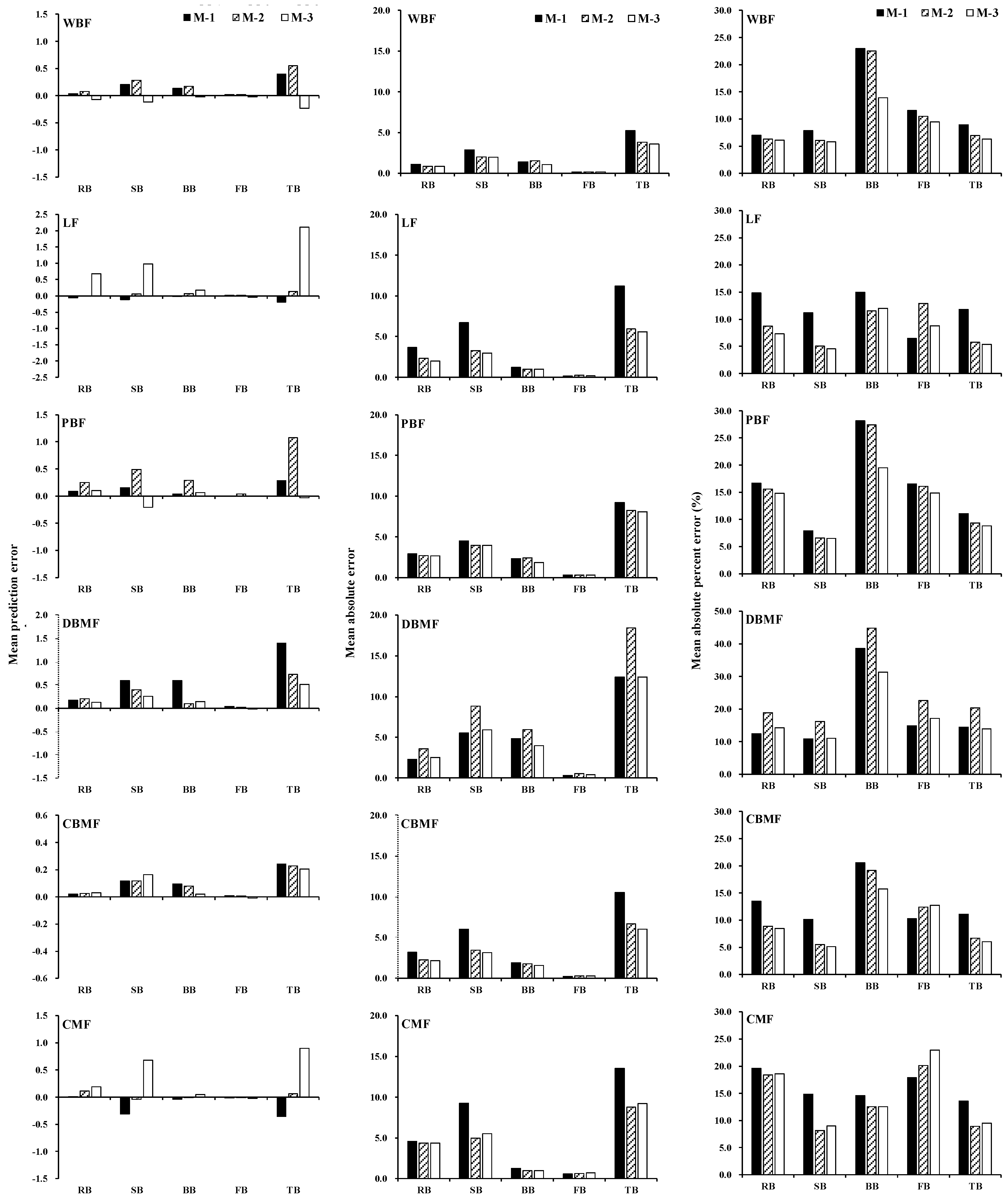
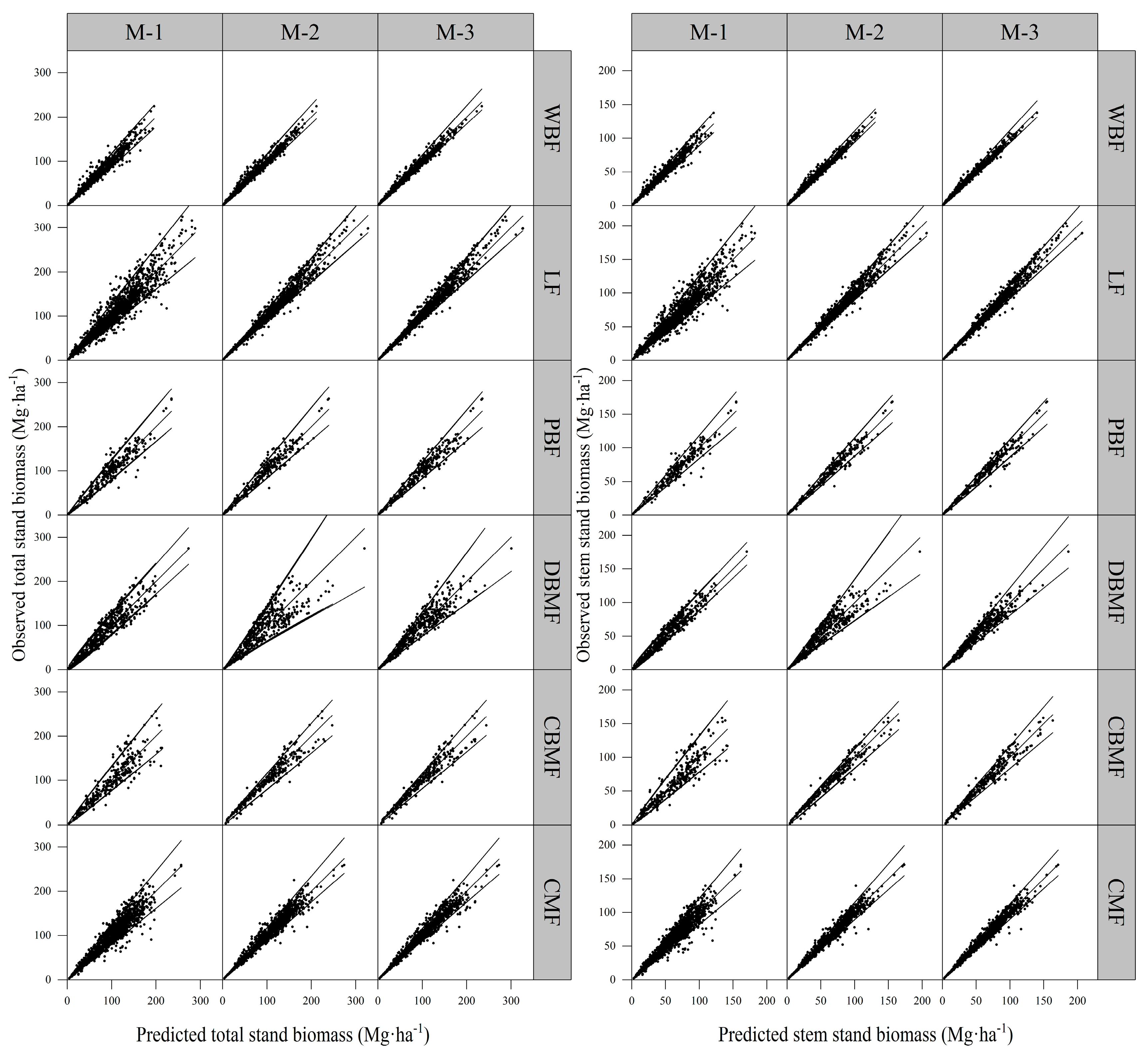
3.2. Model Validation for Stand Biomass Models

The model validation statistics (Equations (9)–(13)) for M-1, M-2, and M-3 were computed. For most stand biomass models, the MPE was close to 0, the MAE was relatively small (< 20 Mg·ha⁻¹), the MAE% was less than 30%, and M-2 and M-3 seemed preferable to M-1. For the stand total biomass, relatively small model prediction errors were reported for three of the systems in all forest types, except deciduous broadleaf mixed forest, and M-3 and M-2 seemed to be better than M-1, which was also found for the stand stem biomass (Figure 2). On the other hand, the stand biomass equations for root, branch, and foliage had less accurate predictions than the total and stem models, especially the branch biomass models.

To quantify the contributions of the variations in the observed stand biomass to the model predictions, the residual and approximate confidence bands of the observed data containing approximately 90% of the average curve were derived for all additive systems of stand biomass equations. The specific methods used to calculate the approximate confidence band were detailed in Bi et al. [36]. Since the relative proportion of stand stem biomass was large for the six forest types, Figure 3 shows only the observed stand total and stem biomasses for the six forest types plotted against their predicted values from M-1, M-2 and M-3. The incorporation of V and BCEF as the predictors in M-3 led to slightly narrower confidence bands for the stand biomass than in M-1 (with G and $H_a$ as the predictors). In general, M-3 predicted the stand total biomass and all components very well for the six forest types.

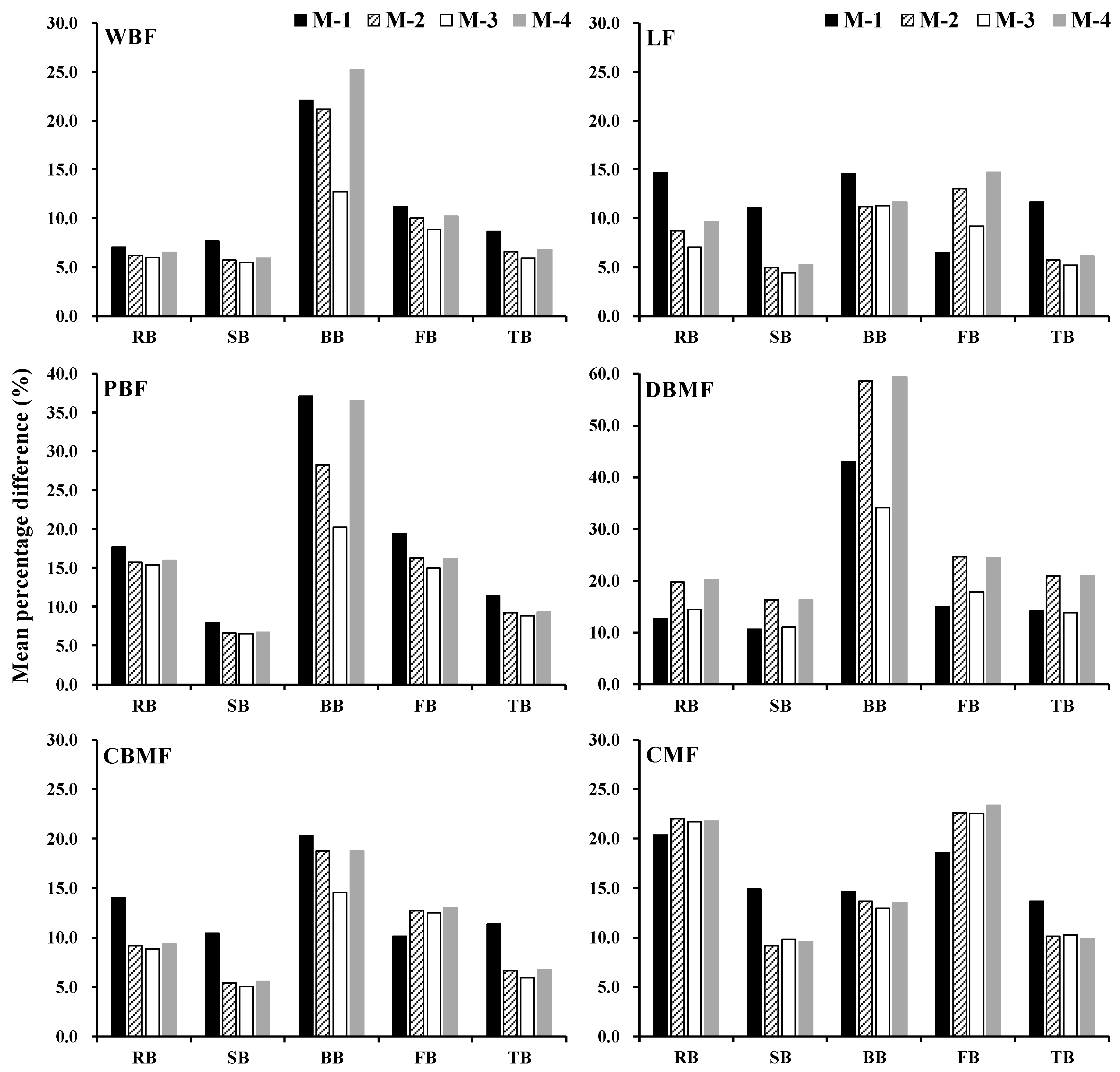
3.3. Comparison of Methods for Estimating Stand Biomass

The analysis of variance was performed to compare the performance of the four estimation methods (i.e., M-1, M-2, M-3, and M-4) in estimating stand biomass, where the four methods were the treatment, and the sample plots served as the blocks (Table 6). The results showed that there were remarkable differences in the stand total and component biomasses among the four methods for white birch forest, larch forest, poplar-birch forest, and deciduous broadleaf mixed forest (Table 6), although significant differences were not observed between the four methods for the stand total, root, stem, and branch biomass models of coniferous and broadleaf mixed forest or for the stand root and branch biomass models of coniferous mixed forest (Table 6).

Furthermore, the percentage difference (MPD%) between the stand total biomass and component biomasses estimated by the four methods was calculated (Figure 4). The results showed that the MPD% between the stand total biomass and components in M-3 was small. However, the MPD% of M-1 was slightly larger than that of the other three methods in all forest types except deciduous broadleaf mixed forest. The overall ranking based on MPD% obeyed the following order: M-3 > M-2 > M-4 > M-1.

4. Discussion

Stand total and component biomasses are frequently estimated using stand variables, which are usually easy to obtain via field investigations. In recent studies on stand biomass estimations, typical allometric equations based on the power-law model are often applied to increase the prediction accuracy of stand biomass [6,7,8,16]. In our M-1 model system, the stand basal area $G$ was a significant and important predictor for the stand total and component biomasses of the six forest types, which confirmed its role in previous studies [6,7]. The estimated coefficients of the stand basal area were positive, indicating that the stand biomass increased as the stand basal area increased. However, for the same stand basal area, large variations occurred among the stand total and component biomasses. Therefore, to improve the prediction accuracy of the stand biomass models, other stand variables should be considered. Previous studies have verified that the dominant height of the stand was the second most important stand variable because it reflected the site quality [7,19]. Unfortunately, the stand dominant height was not available in our data from the permanent sample plots of the NFCI. Instead, we used the average stand height H_a, which was statistically significant for most stand root, stem, branch, and foliage biomass models. As a result, we strongly suggest that future studies on stand biomass consider and investigate the effects of the stand average height or dominant height in the stand biomass models. Other stand variables, such as stand density and stand age, were also included in some stand component biomass equations, and they were commonly considered to represent the competition within a stand and the stage of stand development [6]. The effects of stand density and stand age on some biomass components, such as stem or foliage, are statistically significant and widely recognized, which is likely due to their impacts on branching characteristics and biomass partitioning among the tree components [6,37]. However, the six forest types in this study were natural forests in the Eastern Da Xing’an Mountains. Therefore, they were not good choices for estimating stand biomass. In addition, information on silvicultural practices, such as thinning and tending, was not available, which may affect stand biomass accumulation and allocation and result in biased stand biomass estimations [38].

Many studies indicate that there is a strong correlation between stand biomass and stand volume [20,21,22]. For most forest types, a linear relationship between stand biomass and stand volume is obviously insufficient and controversial. Thus, many researchers have used nonlinear models to describe the relationship and improve model fitting [7,15,16,17,24]. As expected, $\mathrm{BCEF}$ was not constant over stand development in different forest types (Table 2). Thus, using constant $\mathrm{BCEF}$ values would provide biased estimations of stand biomass. In this study, Equations (5) and (6) were used to model the $\mathrm{BCEF}$ variations, which is consistent with the methods used in other studies in the literature. In addition, some studies used stand age as a predictor for modeling BCEF [15,39,40,41]. Although the stand age was unavailable in this study, the stand variables (e.g., H_a and D_q) used in our model systems were indirect surrogates for stand development to a certain extent.

Parresol [28] noted that the aggregation approach is the standard method for ensuring the additivity of estimates of stand total and component biomasses. In Parresol’s method, a nonlinear model is assigned to each of the stand biomass components before aggregating the biomasses of these stand components into the stand total biomass. Notably, if the same predictor variables are used for modeling all stand biomass components, and the same weights are chosen for heteroscedasticity in the model residuals, NSUR will produce singular covariance matrices that do not guarantee a unique solution. Thus, when the same or different predictor variables are considered, the heteroscedasticity of the model residuals should be overcome by different sets of weights, and NSUR is a feasible parameter estimation method [12,42]. The aggregative models in this study were estimated using a weighted NSUR with different weight functions to explain the inherent correlations among the stand component biomasses in the same sample plot [11,12,13,27,28]. Unfortunately, some nonadditive stand biomass models are still published because of the use of the ordinary least-squares regression (OLS) estimation method [8,10].

We evaluated different methods for quantifying stand biomass, and the results were nonconclusive. The results indicated that, except for deciduous broadleaf mixed forest, M-3 performed better than other models, especially for stand total and stem biomass. The reason for this finding may be that there is a close relationship between stand volume and stem biomass, and a higher proportion of stem biomass is included in the total biomass [7,43]. If the stand volume is not available, M-1 will be an effective method to accurately estimate the stand total and component biomasses. For the deciduous broadleaf mixed forest, the stand biomass models with stand variables (M-1) were generally less biased than those obtained from the stand biomass models with stand volume (M-2) or stand volume and BCEF (M-3). The poor performance of the latter two additive models may be the result of the biases after modeling $\mathrm{BCEF}$ by using the stand variables. Many studies have shown that using a constant BCEF to quantify stand biomass introduces certain biases or errors in stand biomass or carbon estimations so that the development of $\mathrm{BCEF}$ models is recommended when the data are available [16]. Generally, $\mathrm{BCEFs}$ vary depending on the growth conditions and stand development stage expressed by the age and size of the stand [10,15,16,17,41]. Thus, it is easy to understand that M-4 exhibited a worse prediction accuracy than M-2 and M-3. In general, both M-2 and M-3 are stand biomass estimations method based on stand volume, which is essentially different from M-1 [44,45,46]. Overall, the use of M-1, M-2, and M-3 in conjunction with stand growth and yield models would be useful for the growth predictions of the six forest types in response to changes in stand conditions and is appropriate for sustainable forest ecosystem management studies.

To date, few studies have developed individual tree biomass equations for the major forest species in the Eastern Da Xing’an Mountains, Northeast China [14]. However, the data required to apply these equations are not always available. In addition, some growth models for the six forest types in the region were previously developed at Northeast Forestry University, China, which mainly calculated the stand variables, such as $G$ and $V$. For the stand biomass estimations, the use of stand variables can likely avoid the need to address complex error propagation procedures for stand biomass estimations at different spatial scales [7]. Although estimating the stand biomass using stand variables may produce some differences in the tree-based biomass estimation, the differences seem acceptable at the forest or stand level for a large geographic region. Thus, the stand biomass models using stand variables (e.g., $G$, $V$, $H_a$, and $D_q$) would be useful, convenient, and efficient.

5. Conclusions

Our study provided a comprehensive overview of the methods used to estimate the aboveground and belowground stand biomass of the six major forest types in the eastern Da Xing’an Mountains, Northeast China. Three additive systems of stand biomass equations were developed and evaluated: the stand biomass models using stand variables (M-1), the stand biomass models using stand volume (M-2), and the stand biomass models using both stand volume and $\mathrm{BCEF}$ (M-3). In these three model systems, the inherent correlation between stand total biomass and component biomass was constrained by applying NSUR for the model parameter estimation. We also comprehensively evaluated four stand biomass estimation methods (i.e., the three additive systems and constant BCEF (M-4)). The results indicated that the model fitting and validation of M-3, which included both stand volume and BCEF, were better than those of M-1 and M-2. Overall, the four methods showed good accuracy in estimating stand total and component biomasses for the six major forest types in the region. However, the choice of methods depends on the available data. If the stand volume is not known, then the stand biomass can be estimated using stand variables, such as $G$ and $H_a$. However, caution should be used when predicting stand total and component biomasses outside the data range used in this study.

References

1. Canadell, J.G.; Raupach, M.R. Managing forests for climate change mitigation. Science 2008, 320, 1456–1457. [Google Scholar] [CrossRef] [PubMed]
2. Pan, Y.; Birdsey, R.A.; Fang, J.; Houghton, R.; Kauppi, P.E.; Kurz, W.A.; Phillips, O.L.; Shvidenko, A.; Lewis, S.L.; Canadell, J.G. A large and persistent carbon sink in the world’s forests. Science 2011, 333, 988–993. [Google Scholar] [CrossRef] [PubMed]
3. Foster, J.R.; Finley, A.O.; D’amato, A.W.; Bradford, J.B.; Banerjee, S. Predicting tree biomass growth in the temperate–boreal ecotone: Is tree size, age, competition, or climate response most important? Glob. Chang. Biol. 2016, 22, 2138–2151. [Google Scholar] [CrossRef] [PubMed]
4. Kachamba, D.; Eid, T.; Gobakken, T. Above-and belowground biomass models for trees in the miombo woodlands of Malawi. Forests 2016, 7, 38. [Google Scholar] [CrossRef]
5. Kapinga, K.; Syampungani, S.; Kasubika, R.; Yambayamba, A.M.; Shamaoma, H. Species-specific allometric models for estimation of the above-ground carbon stock in miombo woodlands of Copperbelt Province of Zambia. For. Ecol. Manag. 2018, 417, 184–196. [Google Scholar] [CrossRef]
6. Bi, H.; Long, Y.; Turner, J.; Lei, Y.; Snowdon, P.; Li, Y.; Harper, R.; Zerihun, A.; Ximenes, F. Additive prediction of aboveground biomass for Pinus radiata (D. Don) plantations. For. Ecol. Manag. 2010, 259, 2301–2314. [Google Scholar] [CrossRef]
7. Castedo-Dorado, F.; Gómez-García, E.; Diéguez-Aranda, U.; Barrio-Anta, M.; Crecente-Campo, F. Aboveground stand-level biomass estimation: A comparison of two methods for major forest species in northwest Spain. Ann. For. Sci. 2012, 69, 735–746. [Google Scholar] [CrossRef]
8. Paré, D.; Bernier, P.; Lafleur, B.; Titus, B.D.; Thiffault, E.; Maynard, D.G.; Guo, X. Corrigendum: Estimating stand-scale biomass, nutrient contents, and associated uncertainties for tree species of Canadian forests. Can. J. For. Res. 2013, 43, 1084. [Google Scholar] [CrossRef]
9. Di Cosmo, L.; Gasparini, P.; Tabacchi, G. A national-scale, stand-level model to predict total above-ground tree biomass from growing stock volume. For. Ecol. Manag. 2016, 361, 269–276. [Google Scholar] [CrossRef]
10. Jagodziński, A.; Dyderski, M.; Gęsikiewicz, K.; Horodecki, P. Tree-and Stand-Level Biomass Estimation in a Larix decidua Mill. Chronosequence. Forests 2018, 9, 587. [Google Scholar] [CrossRef]
11. Bi, H.; Turner, J.; Lambert, M.J. Additive biomass equations for native eucalypt forest trees of temperate Australia. Trees 2004, 18, 467–479. [Google Scholar] [CrossRef]
12. Dong, L.; Zhang, L.; Li, F. Developing additive systems of biomass equations for nine hardwood species in Northeast China. Trees 2015, 29, 1149–1163. [Google Scholar] [CrossRef]
13. Zhao, D.; Kane, M.; Markewitz, D.; Teskey, R.; Clutter, M. Additive tree biomass equations for midrotation loblolly pine plantations. For. Sci. 2015, 61, 613–623. [Google Scholar] [CrossRef]
14. Dong, L.; Zhang, L.; Li, F. Additive biomass equations based on different dendrometric variables for two dominant species (Larix gmelini Rupr. and Betula platyphylla Suk.) in natural forests in the eastern Daxing’an Mountains, Northeast China. Forests 2018, 9, 261. [Google Scholar] [CrossRef]
15. Teobaldelli, M.; Somogyi, Z.; Migliavacca, M.; Usoltsev, V.A. Generalized functions of biomass expansion factors for conifers and broadleaved by stand age, growing stock and site index. For. Ecol. Manag. 2009, 257, 1004–1013. [Google Scholar] [CrossRef]
16. González-García, M.; Hevia, A.; Majada, J.; Barrio-Anta, M. Above-ground biomass estimation at tree and stand level for short rotation plantations of Eucalyptus nitens (Deane & Maiden) Maiden in Northwest Spain. Biomass Bioenergy 2013, 54, 147–157. [Google Scholar]
17. Jagodziński, A.M.; Dyderski, M.K.; Gęsikiewicz, K.; Horodecki, P.; Cysewska, A.; Wierczyńska, S.; Maciejczyk, K. How do tree stand parameters affect young Scots pine biomass?—Allometric equations and biomass conversion and expansion factors. For. Ecol. Manag. 2018, 409, 74–83. [Google Scholar] [CrossRef]
18. Liu, J.; Hyyppa, J.; Yu, X.; Jaakkola, A.; Kukko, A.; Kaartinen, H.; Zhu, L.; Liang, X.; Wang, Y.; Hyyppa, H. A novel GNSS technique for predicting boreal forest attributes at low cost. IEEE Trans. Geosci. Remote 2017, 55, 4855–4867. [Google Scholar] [CrossRef]
19. Wang, X.; Ouyang, S.; Sun, O.J.; Fang, J. Forest biomass patterns across northeast China are strongly shaped by forest height. For. Ecol. Manag. 2013, 293, 149–160. [Google Scholar] [CrossRef]
20. Fang, J.-Y.; Wang, G.G.; Liu, G.-H.; Xu, S.-L. Forest biomass of China: An estimate based on the biomass–volume relationship. Ecol. Appl. 1998, 8, 1084–1091. [Google Scholar]
21. Luo, Y.; Wang, X.; Zhang, X.; Ren, Y.; Poorter, H. Variation in biomass expansion factors for China’s forests in relation to forest type, climate, and stand development. Ann. For. Sci. 2013, 70, 589–599. [Google Scholar] [CrossRef]
22. Pan, Y.; Luo, T.; Birdsey, R.; Hom, J.; Melillo, J. New estimates of carbon storage and sequestration in China’s forests: Effects of age–class and method on inventory-based carbon estimation. Clim. Chang. 2004, 67, 211–236. [Google Scholar] [CrossRef]
23. IPCC. 2006 IPCC Guidelines for National Greenhouse Gas Inventories; Institute for Global Environmental Strategies: Kanagawa, Japan, 2006. [Google Scholar]
24. Zhou, G.; Wang, Y.; Jiang, Y.; Yang, Z. Estimating biomass and net primary production from forest inventory data: A case study of China’s Larix forests. For. Ecol. Manag. 2002, 169, 149–157. [Google Scholar] [CrossRef]
25. Zhao, M.; Zhou, G.S. Estimation of biomass and net primary productivity of major planted forests in China based on forest inventory data. For. Ecol. Manag. 2005, 207, 295–313. [Google Scholar] [CrossRef]
26. Soares, P.; Tomé, M. Analysis of the Effectiveness of Biomass Expansion Factors to Estimate Stand Biomass. Available online: https://www.researchgate.net/profile/Margarida_Tome3/publication/266016805_Analysis_of_the_effectiveness_of_biomass_expansion_factors_to_estimate_stand_biomass/links/54b5aac30cf28ebe92e799a8.pdf (accessed on 19 July 2019).
27. Parresol, B.R. Assessing tree and stand biomass: A review with examples and critical comparisons. For. Sci. 1999, 45, 573–593. [Google Scholar]
28. Parresol, B.R. Additivity of nonlinear biomass equations. Can. J. For. Res. 2001, 31, 865–878. [Google Scholar] [CrossRef]
29. Tang, S.; Li, Y.; Wang, Y. Simultaneous equations, error-in-variable models, and model integration in systems ecology. Ecol. Model. 2001, 142, 285–294. [Google Scholar] [CrossRef]
30. Zhao, D.; Westfall, J.; Coulston, J.W.; Lynch, T.B.; Bullock, B.P.; Montes, C.R. Additive biomass equations for slash pine trees: Comparing three modeling approaches. Can. J. For. Res. 2018, 49, 27–40. [Google Scholar] [CrossRef]
31. Clifford, D.; Cressie, N.; England, J.R.; Roxburgh, S.H.; Paul, K.I. Correction factors for unbiased, efficient estimation and prediction of biomass from log–log allometric models. For. Ecol. Manag. 2013, 310, 375–381. [Google Scholar] [CrossRef]
32. Dong, L.; Zhang, L.; Li, F. A three-step proportional weighting system of nonlinear biomass equations. For. Sci. 2014, 61, 35–45. [Google Scholar] [CrossRef]
33. Dong, L.; Zhang, L.; Li, F. A compatible system of biomass equations for three conifer species in Northeast, China. For. Ecol. Manag. 2014, 329, 306–317. [Google Scholar] [CrossRef]
34. Balboa-Murias, M.A.; Rodríguez-Soalleiro, R.; Merino, A.; Álvarez-González, J.G. Temporal variations and distribution of carbon stocks in aboveground biomass of radiata pine and maritime pine pure stands under different silvicultural alternatives. For. Ecol. Manag. 2006, 237, 29–38. [Google Scholar] [CrossRef]
35. SAS Institute Inc. SAS/ETS 9.3 User’s Guide; SAS Institute Inc.: Cary, NC, USA, 2011. [Google Scholar]
36. Bi, H.; Murphy, S.; Volkova, L.; Weston, C.; Fairman, T.; Li, Y.; Law, R.; Norris, J.; Lei, X.; Caccamo, G. Additive biomass equations based on complete weighing of sample trees for open eucalypt forest species in south-eastern Australia. For. Ecol. Manag. 2015, 349, 106–121. [Google Scholar] [CrossRef]
37. António, N.; Tomé, M.; Tomé, J.; Soares, P.; Fontes, L. Effect of tree, stand, and site variables on the allometry of Eucalyptus globulus tree biomass. Can. J. For. Res. 2007, 37, 895–906. [Google Scholar] [CrossRef]
38. Albaugh, T.J.; Bergh, J.; Lundmark, T.; Nilsson, U.; Stape, J.L.; Allen, H.L.; Linder, S. Do biological expansion factors adequately estimate stand-scale aboveground component biomass for Norway spruce? For. Ecol. Manag. 2009, 258, 2628–2637. [Google Scholar] [CrossRef]
39. Jenkins, J.C.; Chojnacky, D.C.; Heath, L.S.; Birdsey, R.A. National-scale biomass estimators for United States tree species. For. Sci. 2003, 49, 12–35. [Google Scholar]
40. Lehtonen, A.; Mäkipää, R.; Heikkinen, J.; Sievänen, R.; Liski, J. Biomass expansion factors (BEFs) for Scots pine, Norway spruce and birch according to stand age for boreal forests. For. Ecol. Manag. 2004, 188, 211–224. [Google Scholar] [CrossRef]
41. Jagodziński, A.M.; Zasada, M.; Bronisz, K.; Bronisz, A.; Bijak, S. Biomass conversion and expansion factors for a chronosequence of young naturally regenerated silver birch (Betula pendula Roth) stands growing on post-agricultural sites. For. Ecol. Manag. 2017, 384, 208–220. [Google Scholar] [CrossRef]
42. Goicoa, T.; Militino, A.; Ugarte, M. Modelling aboveground tree biomass while achieving the additivity property. Environ. Ecol. Stat. 2011, 18, 367–384. [Google Scholar] [CrossRef]
43. Bi, H.; Birk, E.; Turner, J.; Lambert, M.; Jurskis, V. Converting stem volume to biomass with additivity, bias correction, and confidence bands for two Australian tree species. N. Z. J. For. Sci. 2001, 31, 298–319. [Google Scholar]
44. Wang, X.; Feng, Z.; Ouyang, Z. The impact of human disturbance on vegetative carbon storage in forest ecosystems in China. For. Ecol. Manag. 2001, 148, 117–123. [Google Scholar] [CrossRef]
45. Li, H.; Zhao, P.; Lei, Y.; Zeng, W. Comparison on estimation of wood biomass using forest inventory data. Sci. Silvae Sin. 2012, 48, 44–52. [Google Scholar]
46. Fang, J.; Chen, A.; Peng, C.; Zhao, S.; Ci, L. Changes in forest biomass carbon storage in China between 1949 and 1998. Science 2001, 292, 2320–2322. [Google Scholar] [CrossRef] [PubMed]
Figure 1. Geographical location of the study area in the Eastern Da Xing’an Mountains, Northeast China.
Forests 10 00715 g001
Figure 2. Mean prediction error (MPE), mean absolute error (MAE) and mean absolute percent error (MAE%) among the total and component biomasses for each forest type. WBF, LF, PBF, DBMF, CBMF and CMF stand for white birch forest, larch forest, poplar-birch forest, deciduous broadleaf mixed forest, coniferous and broadleaf mixed forest and coniferous mixed forest, respectively. TB, RB, SB, BB and FB represent the total, root, stem, branch, and foliage biomass, respectively.
Forests 10 00715 g002
Figure 3. Multipanel display of observed total and stem biomass for each forest type plotted against their predicted values from M-1, M-2 and M-3. The diagonal line of unity is shown with the 90% upper and lower confidence limits of prediction error in each panel.
Forests 10 00715 g003
Figure 4. The mean percentage differences of the four methods used to estimate stand biomass for each forest type. WBF, LF, PBF, DBMF, CBMF and CMF stand for white birch forest, larch forest, poplar-birch forest, deciduous broadleaf mixed forest, coniferous and broadleaf mixed forest and coniferous mixed forest, respectively. TB, RB, SB, BB and FB represent the total, root, stem, branch and foliage biomass, respectively.
Forests 10 00715 g004