Estimation of Forest Biomass and Carbon Storage in China Based on Forest Resources Inventory Data


Abstract
:1. Introduction
2. Materials and Methods
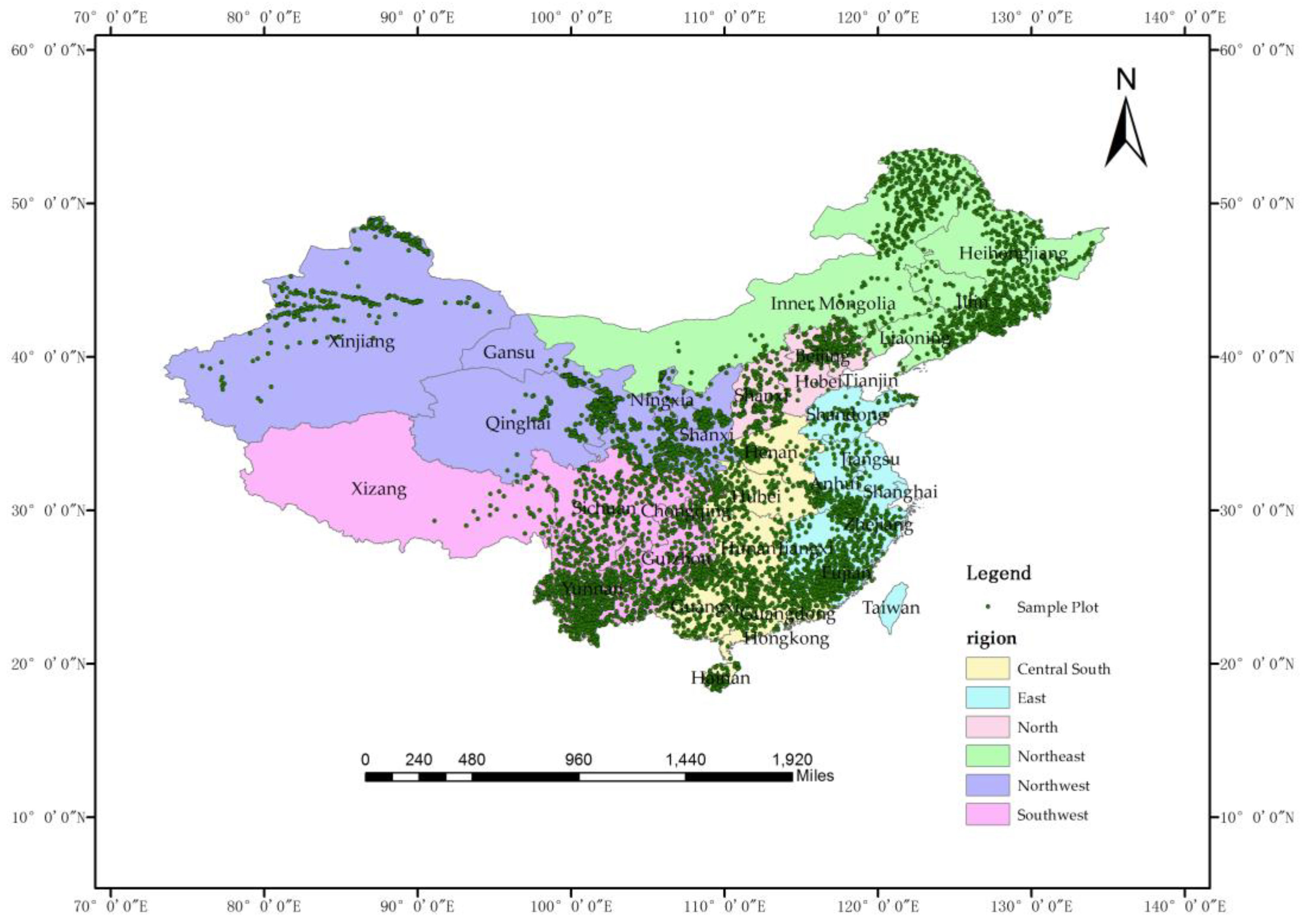
2.1. Data Collection
2.2. Method of Stand Volume Model Establishing
2.3. Model Evaluation and Validation
2.4. Methods of Aboveground Biomass (AGB) and Aboveground Carbon (AGC) Estimation
3. Results
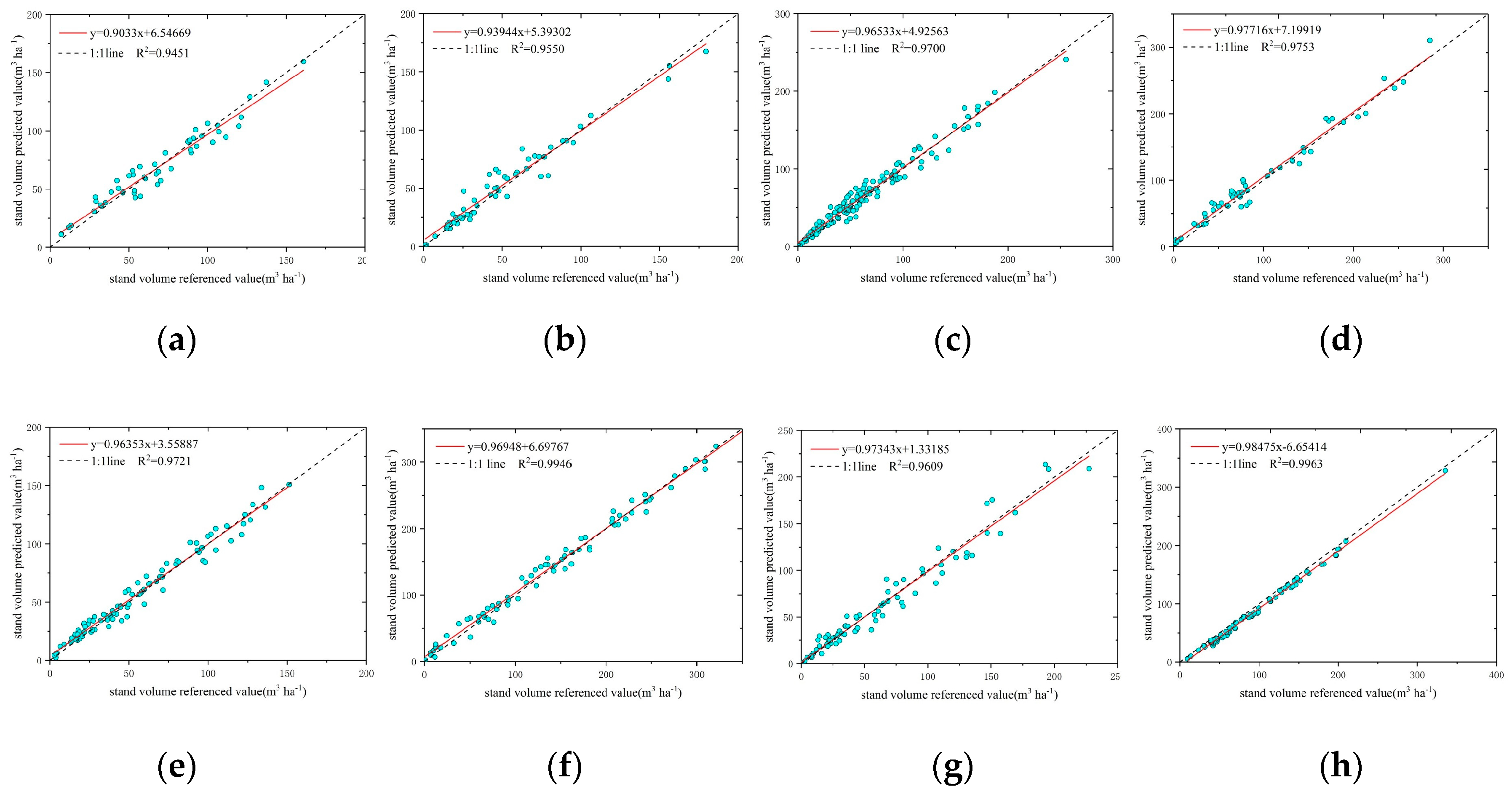
3.1. Result of Stand Volume Model Establishment
3.2. Model Precision Evaluation
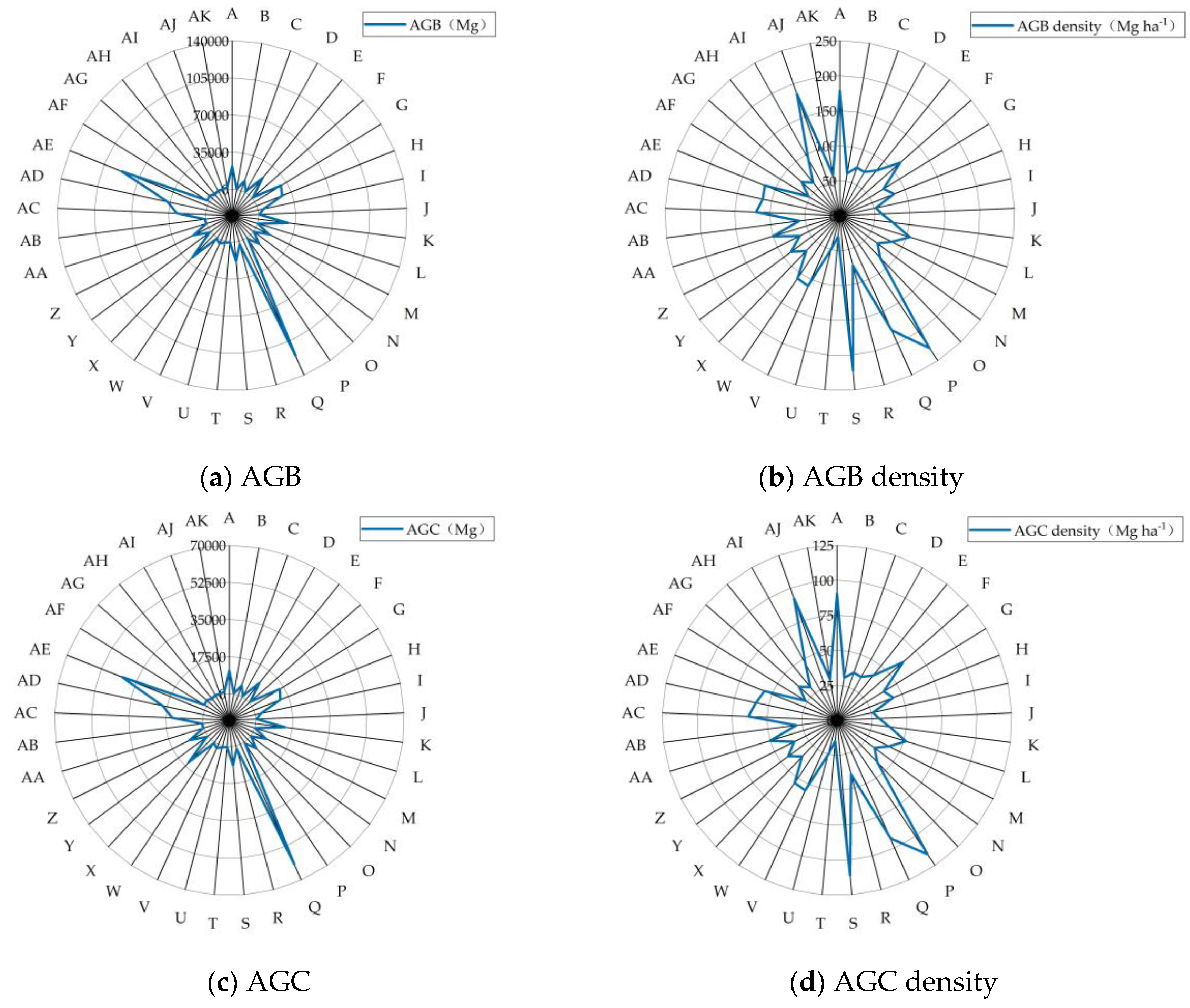
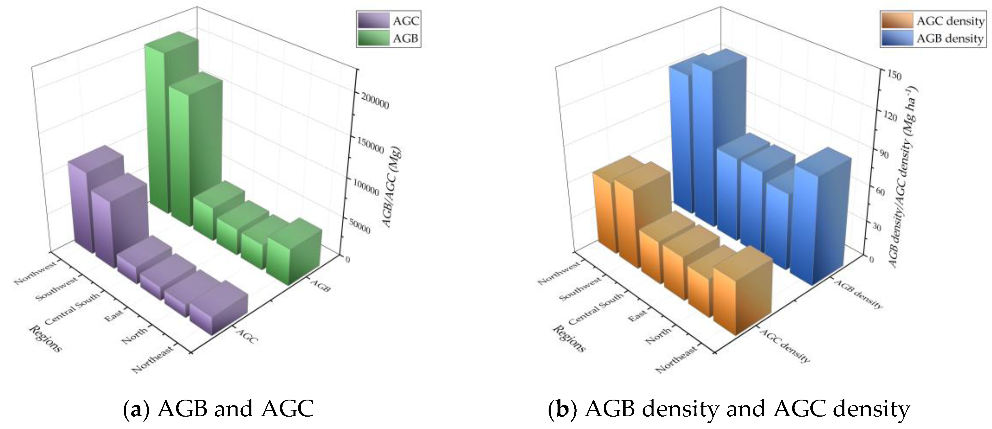
3.3. Results of Aboveground Biomass (AGB) and Aboveground Carbon (AGC) for Different Forest Types in China
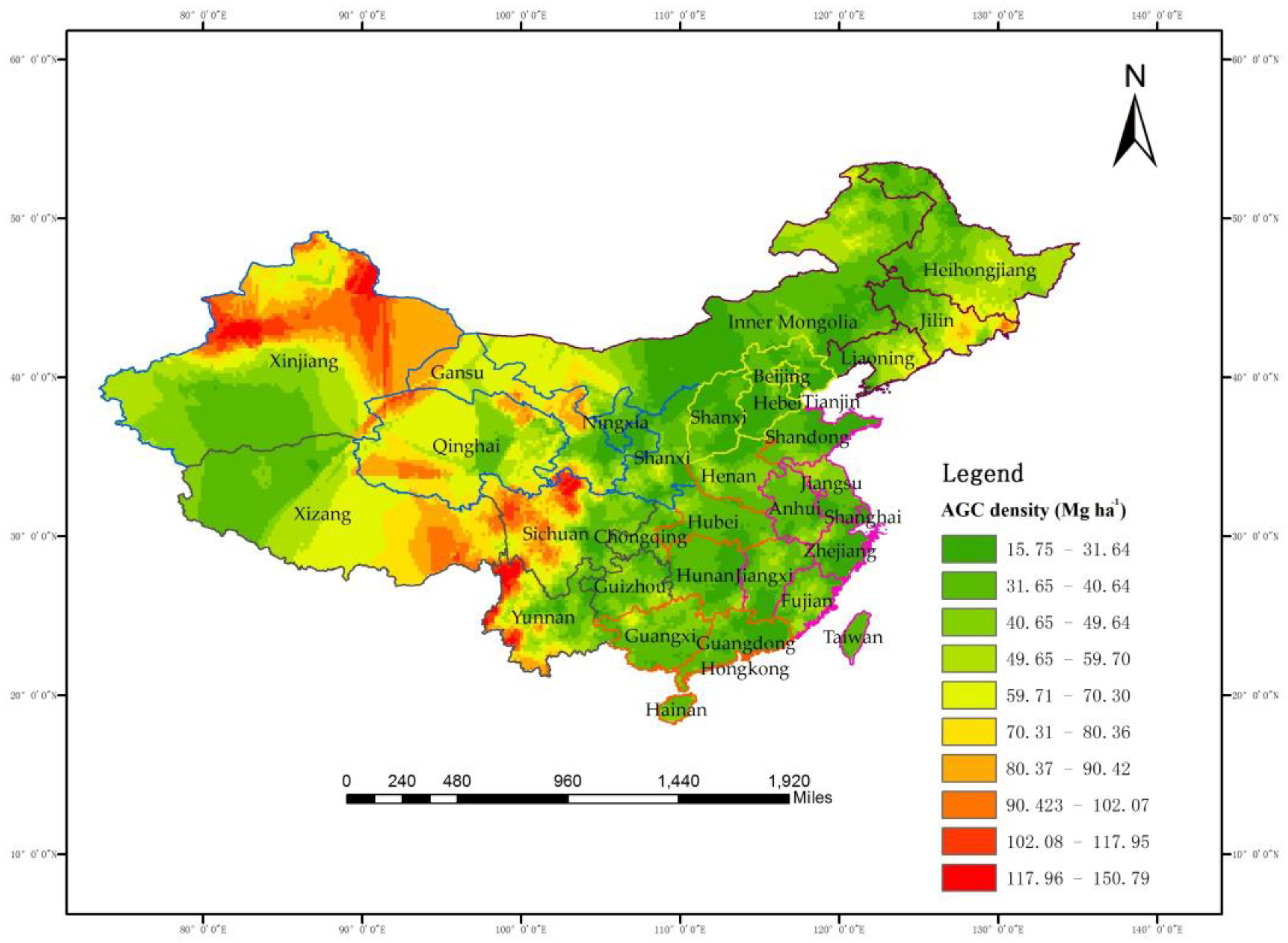
3.4. Spatial Distribution of Forest Aboveground Biomass (AGB) and Aboveground Carbon (AGC) in China
4. Discussion
5. Conclusions
Supplementary Materials
Author Contributions
Funding
Acknowledgments
Conflicts of Interest
Appendix A

| Provinces | Sub-Pop. | Area (ha) | Grid (km) | Plot Shape | Plot Size (ha) |
|---|---|---|---|---|---|
| Beijing | / | 16,410 | 2 × 2 | Square | 0.0667 |
| Tianjin | / | 11,305 | 2 × 2 | Square | 0.0667 |
| Hebei | / | 187,693 | 4 × 4 | Square | 0.06 |
| Shanxi | / | 156,623 | 4 × 4 | Square | 0.0667 |
| InnerMongolia | / | 11,830 | 8 × 8 | Rectangular | 0.06 |
| Liaoning | / | 145,739 | 4 × 8 | Square | 0.08 |
| Jilin | / | 189,193 | 4 × 16/3 | Square | 0.06 |
| Heilongjiang | I | 100,540 | 8 × 8 | Square | 0.06 |
| II | 64,786 | 8 × 8 | Rectangular | 0.06 | |
| III | 289,282 | 4 × 8 | Square | 0.06 | |
| Shanghai | / | 6341 | 2 × 1 | Square | 0.0667 |
| Jiangsu | / | 102,600 | 4 × 3 | Square | 0.0667 |
| Zhejiang | / | 101,800 | 4 × 6 | Square | 0.08 |
| Anhui | / | 138,165 | 4 × 3 | Square | 0.0667 |
| Fujian | / | 121,501 | 4 × 6 | Square | 0.0667 |
| Jiangxi | / | 166,946 | 8 × 8 | Square | 0.0667 |
| Shandong | / | 152,221 | 4 × 4 | Square | 0.0667 |
| Henan | / | 167,000 | 4 × 4 | Square | 0.08 |
| Hubei | / | 185,900 | 4 × 8 | Square | 0.0667 |
| Hunan | / | 211,835 | 4 × 8 | Square | 0.0667 |
| Guangdong | / | 176,769 | 6 × 8 | Square | 0.0667 |
| Guangxi | / | 237,600 | 6 × 8 | Square | 0.0667 |
| Hainan | / | 33,907 | 4 × 3 | Square | 0.0667 |
| Chongqing | / | 82,335 | 4 × 4 | Square | 0.0667 |
| Sichuan | / | 483,744 | 6 × 8 | Square | 0.0667 |
| Guizhou | / | 176,167 | 4 × 8 | Square | 0.0667 |
| Yunnan | / | 382,644 | 6 × 8 | Square | 0.0667 |
| Xizang | / | 1,228,436 | 6 × 8 | Circular | 0.0667 |
| Shaanxi | / | 205,977 | 4 × 8 | Square | 0.08 |
| Gansu | I | 449,734 | 2 × 3 | Square | 0.08 |
| II | 3 × 3 | Square | 0.08 | ||
| III | 4 × 8 | Square | 0.08 | ||
| Qinghai | I | 721,514 | 2 × 2 | Square | 0.08 |
| II | 4 × 2 | Square | 0.08 | ||
| Ningxia | / | 51,955 | 2 × 2 | Square | 0.06 |
| Xinjiang | I | 164,700 | 3 × 4 | Square | 0.08 |
| II | 6 × 4 | Square | 0.08 |
| Group | Forest Type (Dominant Species) | Common Name |
|---|---|---|
| broad-leaved forest | Abies fabri (Mast.) Craib | Acacia rachii |
| Abrus spp. | Birch | |
| Betula spp. | Ribbed Birch | |
| Betula Costata Trautv | White birch | |
| Betula platyphylla Suk. | Eucalyptus | |
| Cryptomeria fortunei Hooibrenk ex Otto et Dietr. | Larch | |
| Cunninghamia lanceolata (Lamb.) Hook. | Camphorwood | |
| Cupressus funebris Endl. | Other hard-and-broad trees | |
| Eucalyptus robusta Smith | Other soft-and-broad trees | |
| Keteleeria fortunei (Murr.) Carr. | Phoebe | |
| Larix gmelinii (Ruprecht) Kuzeneva | Quercus | |
| Cinnamomum camphora (L.) Presl. | Locust | |
| Other hard-and-broad trees | Willow | |
| Other pine trees | Schima | |
| Other soft-and-broad trees | Linden | |
| Phoebe zhennan S. Lee et F. N. Wei | Elm | |
| coniferous forest | Picea asperata Mast. | Fir |
| Pinus armandii Franch. | Japanese cedar | |
| Pinus densata Mast. | China fir | |
| Pinus densiflora Sieb. et Zucc. | Weeping cypress | |
| Pinus elliottii Engelmann | Keteleeria | |
| Pinus kesiya Royle ex Gordon var. langbianensis (A.Chev) Gaussen | Other pine trees | |
| Pinus koraiensis Siebold et Zuccarini | Spruce | |
| Pinus massoniana Lamb. | Pinus armandi | |
| Pinus sylvestris Linn. var. mongolica Litv. | Alpine pine | |
| Pinus tabulaeformis Carr. | Japanese red pine | |
| Pinus taiwanensis Hayata | Sash pine | |
| Pinus thunbergii Parlatore | Simao pine | |
| Pinus yunnanensis Franch. | Korean pine | |
| Populus spp. | Masson pine | |
| Quercus spp. | Mongolian scotch pine | |
| Robinia pseudoacacia Linn. | Chinese pine | |
| Salix spp. | Huangshan Pine | |
| Schima superba Gardn. et Champ. | Lodgepole pine | |
| Tilia tuan Szyszyl. | Yunnan pine | |
| Tsuga chinensis (Franch.) Pritz. | Poplar | |
| Ulmus pumila Linn. | Hemlock |
| Forest Type | n | |||||||
|---|---|---|---|---|---|---|---|---|
| a | SE(a) | b | SE(b) | c | SE(c) | R2 | ||
| Abies fabri (Mast.) Craib | 72 | 3.784 | 3.031 | 1.349 | 0.296 | 0.144 | 0.215 | 0.37 |
| Abrus spp. | 8 | 0.325 | 0.462 | 0.266 | 0.459 | 2.054 | 0.472 | 0.90 |
| Betula spp. | 98 | 1.713 | 0.620 | 1.099 | 0.140 | 0.285 | 0.210 | 0.54 |
| Betula Costata Trautv | 14 | 1.209 | 1.249 | 1.393 | 0.541 | 0.000 | 0.861 | 0.78 |
| Betula platyphylla Suk. | 206 | 2.732 | 0.813 | 0.064 | 0.091 | 1.167 | 0.127 | 0.37 |
| Cryptomeria fortunei Hooibrenk ex Otto et Dietr. | 9 | 8.884 | 8.498 | 0.991 | 0.293 | 0.097 | 0.114 | 0.63 |
| Cunninghamia lanceolata (Lamb.) Hook. | 318 | 2.369 | 0.642 | 1.204 | 0.120 | 0.303 | 0.077 | 0.38 |
| Cupressus funebris Endl. | 219 | 0.613 | 0.155 | 1.027 | 0.091 | 0.895 | 0.103 | 0.62 |
| Eucalyptus robusta Smith | 90 | 1.850 | 0.985 | 0.442 | 0.315 | 0.984 | 0.239 | 0.39 |
| Keteleeria fortunei (Murr.) Carr. | 182 | 21.074 | 30.222 | 0.533 | 0.766 | 0.000 | 0.993 | 0.15 |
| Larix gmelinii (Ruprecht) Kuzeneva | 294 | 2.637 | 0.663 | 0.581 | 0.093 | 0.697 | 0.107 | 0.39 |
| Cinnamomum camphora (L.) Presl. | 4 | 0.376 | 0.962 | 0.000 | 1.239 | 1.950 | 1.110 | 0.96 |
| Other hard-and-broad trees | 134 | 0.162 | 0.069 | 1.693 | 0.101 | 0.543 | 0.202 | 0.65 |
| Other pine trees | 8 | 0.085 | 0.077 | 2.046 | 0.347 | 0.523 | 0.229 | 0.79 |
| Other soft-and-broad trees | 87 | 1.824 | 0.570 | 0.635 | 0.093 | 0.795 | 0.159 | 0.60 |
| Phoebe zhennan S. Lee et F. N. Wei | 6 | 0.022 | 0.181 | 2.383 | 2.306 | 0.786 | 1.051 | 0.64 |
| Picea asperata Mast. | 479 | 5.013 | 0.879 | 1.078 | 0.089 | 0.230 | 0.077 | 0.52 |
| Pinus armandii Franch. | 29 | 6.742 | 5.018 | 1.007 | 0.385 | 0.000 | 0.343 | 0.34 |
| Pinus densata Mast. | 64 | 2.372 | 0.956 | 0.000 | 0.268 | 1.633 | 0.253 | 0.83 |
| Pinus densiflora Sieb. et Zucc. | 11 | 0.546 | 0.579 | 1.457 | 0.303 | 0.457 | 0.487 | 0.83 |
| Pinus elliottii Engelmann | 22 | 2.364 | 3.068 | 1.157 | 0.557 | 0.022 | 0.174 | 0.25 |
| Pinus kesiya Royle ex Gordon var. langbianensis (A.Chev) Gaussen | 28 | 87.330 | 50.705 | 0.150 | 0.278 | 0.002 | 0.273 | 0.02 |
| Pinus koraiensis Siebold et Zuccarini | 8 | 5.134 | 7.262 | 1.167 | 0.821 | 0.000 | 0.417 | 0.60 |
| Pinus massoniana Lamb. | 336 | 4.353 | 0.936 | 0.980 | 0.103 | 0.180 | 0.104 | 0.37 |
| Pinus sylvestris Linn. var. mongolica Litv. | 14 | 1.576 | 1.325 | 1.593 | 0.368 | 0.000 | 0.329 | 0.70 |
| Pinus tabulaeformis Carr. | 11 | 3.047 | 0.797 | 1.383 | 0.131 | 0.000 | 0.137 | 0.55 |
| Pinus taiwanensis Hayata | 4 | 2.709 | 2.253 | 1.585 | 1.618 | 0.023 | 1.218 | 0.95 |
| Pinus thunbergii Parlatore | 14 | 0.258 | 0.433 | 0.067 | 0.571 | 2.085 | 0.907 | 0.53 |
| Pinus yunnanensis Franch. | 184 | 2.120 | 0.444 | 1.677 | 0.144 | 0.000 | 0.151 | 0.80 |
| Populus spp. | 296 | 3.329 | 0.805 | 1.094 | 0.128 | 0.214 | 0.078 | 0.50 |
| Quercus spp. | 578 | 2.168 | 0.379 | 0.535 | 0.077 | 0.931 | 0.095 | 0.44 |
| Robinia pseudoacacia Linn. | 39 | 0.584 | 0.471 | 0.527 | 0.265 | 1.319 | 0.443 | 0.45 |
| Salix spp. | 36 | 0.695 | 0.594 | 0.223 | 0.318 | 1.496 | 0.300 | 0.56 |
| Schima superba Gardn. et Champ. | 16 | 1.369 | 1.174 | 0.231 | 0.426 | 1.382 | 0.332 | 0.76 |
| Tilia tuan Szyszyl. | 18 | 0.042 | 0.064 | 0.470 | 0.773 | 2.421 | 0.692 | 0.68 |
| Tsuga chinensis (Franch.) Pritz. | 6 | 0.085 | 0.127 | 0.948 | 0.965 | 1.486 | 0.963 | 0.94 |
| Ulmus pumila Linn. | 27 | 0.328 | 0.350 | 0.370 | 0.338 | 1.602 | 0.400 | 0.53 |
| Forest Type | ||||||
|---|---|---|---|---|---|---|
| n | BIAS | BIAS% | RMSE | RMSE% | ||
| Abies fabri (Mast.) Craib | 18 | −116.878 | −41.444 | 145.310 | 51.526 | 0.35 |
| Abrus spp. | 2 | −35.023 | −16.856 | 93.724 | 45.108 | 0.57 |
| Betula spp. | 25 | 12.710 | 4.148 | 147.679 | 48.198 | 0.73 |
| Betula Costata Trautv | 3 | −7.225 | −10.302 | 12.595 | 17.959 | 0.21 |
| Betula platyphylla Suk. | 51 | −22.239 | −20.507 | 75.932 | 70.019 | 0.38 |
| Cryptomeria fortunei Hooibrenk ex Otto et Dietr. | 2 | −33.926 | −60.551 | 53.802 | 96.025 | 0.49 |
| Cunninghamia lanceolata (Lamb.) Hook. | 79 | −29.391 | −27.698 | 62.854 | 59.235 | 0.12 |
| Cupressus funebris Endl. | 55 | −12.185 | −69.888 | 15.966 | 91.571 | 0.28 |
| Eucalyptus robusta Smith | 22 | 27.124 | 57.325 | 41.120 | 86.905 | 0.24 |
| Keteleeria fortunei (Murr.) Carr. | 48 | −8.513 | −13.906 | 37.974 | 62.032 | 0.36 |
| Larix gmelinii (Ruprecht) Kuzeneva | 73 | −22.215 | −43.409 | 30.424 | 59.451 | 0.51 |
| Cinnamomum camphora (L.) Presl. | 1 | −16.691 | −24.677 | 42.299 | 62.536 | 0.09 |
| Other hard-and-broad trees | 33 | 4.794 | 3.371 | 54.828 | 38.558 | 0.80 |
| Other pine trees | 2 | −29.521 | −23.042 | 48.311 | 37.709 | 0.04 |
| Other soft-and-broad trees | 22 | 1.103 | 0.425 | 50.061 | 19.268 | 0.82 |
| Phoebe zhennan S. Lee et F. N. Wei | 1 | −0.276 | −0.635 | 22.014 | 50.767 | 0.25 |
| Picea asperata Mast. | 120 | −31.003 | −30.775 | 76.481 | 75.920 | 0.15 |
| Pinus armandii Franch. | 7 | −35.244 | −52.462 | 81.124 | 120.756 | 0.29 |
| Pinus densata Mast. | 16 | −44.018 | −46.639 | 72.459 | 76.775 | 0.02 |
| Pinus densiflora Sieb. et Zucc. | 3 | 25.862 | 14.776 | 95.619 | 54.632 | 0.14 |
| Pinus elliottii Engelmann | 5 | 4.409 | 6.685 | 40.048 | 60.713 | 0.60 |
| Pinus kesiya Royle ex Gordon var. langbianensis (A.Chev) Gaussen | 7 | 11.064 | 11.301 | 51.230 | 52.327 | 0.25 |
| Pinus koraiensis Siebold et Zuccarini | 2 | 0.451 | 0.742 | 35.625 | 58.643 | 0.54 |
| Pinus massoniana Lamb. | 84 | −0.023 | −0.037 | 27.088 | 44.496 | 0.37 |
| Pinus sylvestris Linn. var. mongolica Litv. | 3 | 0.644 | 1.087 | 31.786 | 53.683 | 0.78 |
| Pinus tabulaeformis Carr. | 3 | 8.622 | 10.943 | 84.007 | 106.619 | 0.22 |
| Pinus taiwanensis Hayata | 1 | 2.739 | 0.980 | 149.686 | 53.568 | 0.56 |
| Pinus thunbergii Parlatore | 3 | 8.930 | 21.105 | 20.827 | 49.222 | 0.64 |
| Pinus yunnanensis Franch. | 44 | −9.961 | −68.416 | 12.052 | 82.781 | 0.76 |
| Populus spp. | 74 | −0.636 | −1.653 | 15.097 | 39.261 | 0.73 |
| Quercus spp. | 144 | 8.981 | 19.871 | 30.568 | 67.632 | 0.42 |
| Robinia pseudoacacia Linn. | 10 | 5.616 | 6.835 | 33.256 | 40.473 | 0.64 |
| Salix spp. | 9 | −5.621 | −7.254 | 39.167 | 50.541 | 0.51 |
| Schima superba Gardn. et Champ. | 4 | 8.462 | 8.489 | 50.323 | 50.485 | 0.68 |
| Tilia tuan Szyszyl. | 4 | −1.861 | −3.098 | 36.284 | 60.408 | 0.36 |
| Tsuga chinensis (Franch.) Pritz. | 2 | −10.277 | −15.895 | 31.432 | 48.614 | 0.71 |
| Ulmus pumila Linn. | 7 | −5.441 | −8.807 | 23.782 | 38.495 | 0.38 |
References
- Yang, X.; Wu, B.; Zhang, J.; Lin, D.; Chang, S. Progress of research into carbon fixation and storage of forest ecosystems. J. Beijing Norm. Univ. 2005, 41, 172–177. [Google Scholar]
- Liu, H.; Lei, R. Research Methods and Advances of AGC and Balance in Forest Ecosystems of China. Acta Bot. Boreali-Occident. Sin. 2005, 25, 835–843. [Google Scholar]
- Li, H.; Lei, Y.; Zeng, W. Forest AGC in China Estimated Using Forestry Inventory Data. Sci. Silvae Sin. 2011, 47, 7–12. [Google Scholar]
- Kang, L.; Meng, W.; He, H. Comparative study on stand volume models—Taking middle-aged Chinese fir in Hunan Province State-owned Forest Farm as an example. Trop. For. 2018, 46, 14–18. [Google Scholar]
- Zhang, N.; Feng, Z.; Feng, Y.; Fan, J. Research on coniferous forest volume estimation model for Wangyedian experimental forest farm. J. Cent. South Univ. For. Technol. 2013, 33, 83–87. [Google Scholar]
- Liu, F. Study on the Growth Dynamic Forecast Model of Chinese fir Stand in Fujian Province. For. Prospect Des. 2018, 38, 1–4. [Google Scholar]
- Zeng, W.; Yang, X.; Chen, X. Comparison on Prediction Precision of One-variable and Two-variable Volume Modelson Tree-leveland Stand-level. Cent. South For. Inventory Plan. 2017, 36, 1–6. [Google Scholar]
- Zhou, S. Construction of Precision Analysis Model for Binary Volume and Volume of Forest Trees. Technol. Innov. Appl. 2015, 34, 16–17. [Google Scholar]
- Reis, A.A.D.; Carvalho, M.C.; Mello, J.M.D.; Gomide, L.R.; Filho, A.C.F.; Junior, F.W.A. Spatial prediction of basal area and volume in Eucalyptus stands using Landsat TM data: An assessment of prediction methods. N. Z. J. For. Sci. 2018, 48, 1. [Google Scholar] [CrossRef]
- Zhang, X. Study on the Impact of Terrain on Community Distribution Pattern in Natural Secondary Forest; Northeast Forestry University: Jilin, China, 2007. [Google Scholar]
- Tong, J.; Jin, G.; Li, F.; Jia, W.; Cui, X. AGC density and distribution in soft broad-leaved mixed forest of different age classes in Heilongjiang Province, Northeast China. Chin. J. Ecol. 2014, 33, 3191–3202. [Google Scholar]
- Wang, X.; Qi, G.; Yu, D.; Zhou, L.; Dai, L. AGC, density, and distribution in forest ecosystems in Jilin Province of Northeast China. Chin. J. Appl. Ecol. 2011, 22, 2013–2020. [Google Scholar]
- Wang, W.; Song, L.; Sui, X. Estimation of Forest AGB and Its Temporal and Spatial Distribution Patterns in Maoershan Forest Farm. J. Northeast For. Univ. 2010, 38, 47–49. [Google Scholar]
- Guo, C.; Zhou, Z.; Kang, F.; Sun, J. The alteration of carbon stock of forest ecosystem by tree species composition in Taiyue Mountain. Chin. J. Ecol. 2014, 33, 2012–2018. [Google Scholar]
- Kauppi, P.E.; Mielikã Inen, K.; Kuusela, K. AGB and carbon budget of European forests, 1971 to 1990. Science 1992, 256, 70–74. [Google Scholar] [CrossRef] [PubMed]
- Liu, G.; Fu, G.; Fang, J. Carbon dynamics of Chinese forests and its contribution to global carbon balance. Acta Ecol. Sin. 2000, 5, 733–740. [Google Scholar]
- West, P.W. Tree and Forest Measurement; Springer: Berlin/Heidelberg, Germany, 2005. [Google Scholar]
- Di Cosmo, L.; Gasparini, P.; Tabacchi, G. A national-scale, stand-level model to predict total above-ground tree AGB from growing stock volume. For. Ecol. Manag. 2016, 361, 269–276. [Google Scholar] [CrossRef]
- Fang, J.; Chen, A.; Peng, C.; Zhao, S.; Ci, L. Changes in forest AGB AGC in China between 1949 and 1998. Science 2001, 292, 2320–2322. [Google Scholar] [CrossRef]
- Qiu, Z. Measurement and Statistics of Land-Surface Forest Vegetation Carbon Sink in China. Ph.D. Thesis, Beijing Forestry University, Beijing, China, 2019. [Google Scholar]
- Wang, X.; Feng, Z.; Ou, Z. Vegetation AGC and density of forest ecosystems in China. Chin. J. Appl. Ecol. 2001, 1, 13–16. [Google Scholar]
- Zhao, M.; Zhou, G. AGC of Forest Vegetation and Its Relationship with Climatic Factors. Sci. Geogr. Sin. 2004, 1, 50–54. [Google Scholar]
- Somogyi, Z.; Cienciala, E.; Mäkipää, R.; Muukkonen, P.; Lehtonen, A.; Weiss, P. Indirect methods of large-scale forest AGB estimation. Eur. J. For. Res. 2007, 126, 197–207. [Google Scholar] [CrossRef]
- Zhou, G.; Wang, Y.; Jiang, Y.; Yang, Z. Estimating AGB and net primary production from forest inventory data: A case study of China’s Larix forests. For. Ecol. Manag. 2002, 169, 149–157. [Google Scholar] [CrossRef]
- Fang, J.Y.; Wang, G.G.; Liu, G.H.; Xu, S.L. Forest AGB of China: An estimate based on the AGB–volume relationship. Ecol. Appl. 1998, 8, 1084–1091. [Google Scholar]
- Johnson, W.C.; Sharpe, D.M. The ratio of total to merchantable forest AGB and its application. Revue Can. Rech. For. 1983, 13, 372–383. [Google Scholar] [CrossRef]
- Liu, J.; Feng, Z.; Mannan, A.; Khan, T.; Cheng, Z. Comparing Non-Destructive Methods to Estimate Volume of Three Tree Taxa in Beijing, China. Forests 2019, 10, 92. [Google Scholar] [CrossRef]
- Fang, J.; Liu, G.; Zhu, B.; Wang, X.; Liu, S. Carbon Cycle of Three Temperate Forest Ecosystems in Dongling Mountain, Beijing. Sci. Sin. 2006, 36, 533–543. [Google Scholar]
- Huang, X.; Dai, D.; Huang, C.; Teng, M.; Zhou, Z. Researches Progress in AGB and Productivity of Pinus massoniana. World For. Res. 2019, 32, 53–58. [Google Scholar]
- Guo-Qing, W.; Xue-Feng, C. Studies on stand dynamic growth model for larch in Jilin in China. J. For. Res. 2004, 15, 323–326. [Google Scholar] [CrossRef]
- Shao, W.; Cai, J.; Wu, H.; Liu, J. An Assessment of AGC in China’s Arboreal Forests. Forests 2017, 8, 110. [Google Scholar] [CrossRef]
- LY/T 2188.1-2013, Forest resource data collection technical specification—Part 1: Forest continuous inventory. In Industry Standard—Forestry.
- Knowe, S.A.; Foster, G.S. Application of Growth Models for Simulating Genetic Gain of Loblolly Pine. For. Sci. 1989, 35, 211–228. [Google Scholar]
- Rehfeldt, G.E.; Wykoff, W.R.; Hoff, R.J.; Steinhoff, R.J. Genetic Gains in Growth and Simulated Yield of Pinus monticola. For. Sci. 1991, 37, 326–342. [Google Scholar]
- Buford, M.A.; Burkhart, H.E. Genetic Improvement Effects on Growth and Yield of Loblolly Pine Plantations. For. Sci. 1987, 33, 707–724. [Google Scholar]
- Nance, W.L.; Bay, C.F. Incorporating Genetic Information in Growth and Yield Models. In Proceedings of the 15th Southern Forest Tree Improvement Conference, Starkville, MS, USA, 19–21 June 1979. [Google Scholar]
- Wang, N.; Yang, Y.; Dai, W. The Basal Area Growth Model of Larch Plantation Based on Richards Equation. For. Eng. 2015, 31, 22–25. [Google Scholar]
- Zhang, L.; Hui, G.; Sun, C. Comparison of different stand density measures. J. For. Environ. 2011, 31, 257–261. [Google Scholar]
- Qin, Z.; Dong, W.; Liu, T.; Zhang, Y.; Guo, J.; Wu, Y. Responses of understory plant diversity to stand density in natural secondary forests of Pinus tabulaeformis. J. Shanxi Agric. Univ. (Nat. Sci. Edit.) 2019, 39, 61–67. [Google Scholar]
- LY/T 1353-1999, Standing Volume Table. In Industry Standard-Forestry.
- Maas, D.; Hox, J. The influence of violations of assumptions on multilevel parameter estimates and their standard errors. Comput. Stat. Data Anal. 2003, 46, 427–440. [Google Scholar] [CrossRef]
- Zhang, H.; Feng, Z.; Chen, P.; Chen, X. Development of a Tree Growth Difference Equation and Its Application in Forecasting the AGB Carbon Stocks of Chinese Forests in 2050. Forests 2019, 10, 582. [Google Scholar] [CrossRef]
- Friedlingstein, P.; Cox, P.; Betts, R.; Bopp, L.; Bloh, W.V.; Brovkin, V.; Cadule, P.; Doney, S.; Eby, M.; Fung, I. Climate-Carbon Cycle Feedback Analysis: Results from the C4MIP Model Intercomparison. J. Clim. 2006, 19, 3337–3353. [Google Scholar] [CrossRef]
- Landman, W. Climate change 2007: The physical science basis. S. Afri. Geogr. J. 2007, 92, 86–87. [Google Scholar] [CrossRef]
- Dixon, R.K.; Solomon, A.M.; Brown, S.; Houghton, R.A.; Trexier, M.C.; Wisniewski, J. Carbon pools and flux of global forest ecosystems. Science 1994, 263, 185–190. [Google Scholar] [CrossRef]
- Huang, C.; Zhang, J.; Yang, W.; Tang, X.; Zhao, A. Dynamics on forest carbon stock in Sichuan Province and Chongqing City. Acta Ecol. Sin. 2008, 28, 966–975. [Google Scholar]
- Li, F.; Li, M.; Shi, Z. Estimates Stand Age Distribution Based on Forest Survey and Remote Sensing data. For. Eng. 2018, 34, 30–34. [Google Scholar]
- Zhao, M.; Yue, T.; Zhao, N. Spatial distribution of forest vegetation carbon stock in China based on HASM. Acta Geogr. Sin. 2013, 68, 1212–1224. [Google Scholar]
- Chen, X. Study on the Influencing Factors of Regional Forest Resources Change in China; Beijing Forestry University: Beijing, China, 2007. [Google Scholar]
- Saud, P.; Lynch, T.B.; KC, A.; Guldin, J.M. Using quadratic mean diameter and relative spacing index to enhance height–diameter and crown ratio models fitted to longitudinal data. Forestry 2016, 89, 215–229. [Google Scholar] [CrossRef]
- Sisay, K.; Thurnher, C.; Belay, B.; Lindner, G.; Hasenauer, H. Volume and Carbon Estimates for the Forest Area of the Amhara Region in Northwestern Ethiopia. Forests 2017, 8, 122. [Google Scholar] [CrossRef]
- Zhang, X.; Zhang, J.; Duan, A. Compatibility of Stand Volume Model for Chinese Fir Based on Tree-Level and Stand-Level. Sci. Silvae Sin. 2014, 50, 82–87. [Google Scholar]
- Alexeyev, V.; Birdsey, R.; Stakanov, V.; Korotkov, I. Carbon in vegetation of Russian forests: Methods to estimate storage and geographical distribution. Water Air Soil Pollut. 1995, 82, 271–282. [Google Scholar] [CrossRef]
- Isaev, A.; Korovin, G.; Zamolodchikov, D.; Utkin, A.; Pryaznikov, A. Carbon Stock and Deposition in Phytomass of the Russian Forests. Water Air Soil Pollut. 1995, 82, 247–256. [Google Scholar] [CrossRef]
- Murillo, J.C.R. Temporal Variations in the Carbon Budget of Forest Ecosystems in Spain. Ecol. Appl. 1997, 7, 461–469. [Google Scholar] [CrossRef]
- Harmon, M.E. AGC and Sequestration in the Russian Forest Sector. Ambio 1996, 25, 284–288. [Google Scholar]
- Kurz, W.A.; Apps, M.J.; Webb, T.M.; Mcnamee, P.J. The carbon budget of the Canadian forest sector: Phase I. Simulation 1993, 61, 139–144. [Google Scholar] [CrossRef]
- Heath, L.S.; Kauppi, P.E.; Burschel, P.; Gregor, H.D.; Guderian, R.; Kohlmaier, G.H.; Lorenz, S.; Overdieck, D.; Scholz, F.; Thomasius, H. Contribution of temperate forests to the world’s carbon budget. Water Air Soil Pollut. 1993, 70, 55–69. [Google Scholar] [CrossRef]
- Lin, Q.; Hong, W. Summary of Research on Forest AGC in China. Chin. Agric. Sci. Bull. 2009, 25, 220–224. [Google Scholar]
- Xu, X.; Cao, M.; Li, K. Temporal-Spatial Dynamics of AGC of Forest Vegetation in China. Prog. Geogr. 2007, 6, 1–10. [Google Scholar]
- Bai, Y.; Huang, Y.; Wang, M.; Huang, S.; Sha, C.; Ruan, J. The progress of ecological civilization construction and its indicator system in China. Acta Ecol. Sin. 2011, 31, 6295–6304. [Google Scholar]

| Factors | Number of Data Points (n = 4958) | |||
|---|---|---|---|---|
| Max | Min | Mean | SD | |
| Stand Volume (m3 ha−1) | 1142.61 | 0.06 | 104.91 | 106.63 |
| Mean H (m) | 40.30 | 0.40 | 11.63 | 5.31 |
| Mean DBH (cm) | 85.27 | 5.00 | 15.69 | 7.91 |
| Stand Density (tree ha−1) | 6206.90 | 12.50 | 827.56 | 695.68 |
| Species | ||
|---|---|---|
| Abies fabri (Mast.) Craib | 0.53 | 22.951 |
| Abrus spp. | 0.81 | 10.371 |
| Betula spp. | 0.82 | 18.08 |
| Betula Costata Trautv | 0.93 | 16.459 |
| Betula platyphylla Suk. | 1.33 | −2.881 |
| Cryptomeria fortunei Hooibrenk ex Otto et Dietr. | 0.54 | 20.291 |
| Cunninghamia lanceolata (Lamb.) Hook. | 0.53 | 22.954 |
| Cupressus funebris Endl. | 0.54 | 46.846 |
| Eucalyptus robusta Smith | 0.87 | 1.531 |
| Keteleeria fortunei (Murr.) Carr. | 0.51 | 28.192 |
| Larix gmelinii (Ruprecht) Kuzeneva | 0.92 | −12.64 |
| Other hard-and-broad trees | 0.96 | 29.083 |
| Other pine trees | 0.71 | 18.993 |
| Other soft-and-broad trees | 0.62 | 33.931 |
| Phoebe zhennan S. Lee et F. N. Wei | 0.89 | 28.353 |
| Picea asperata Mast. | 0.48 | 81.143 |
| Pinus armandii Franch. | 0.61 | 29.923 |
| Pinus densata Mast. | 0.81 | 11.892 |
| Pinus densiflora Sieb. et Zucc. | 0.72 | 15.982 |
| Pinus elliottii Engelmann | 0.68 | 19.759 |
| Pinus koraiensis Siebold et Zuccarini | 0.69 | 15.833 |
| Pinus massoniana Lamb. | 0.65 | 25.761 |
| Pinus tabulaeformis Carr. | 0.78 | 13.889 |
| Pinus taiwanensis Hayata | 0.91 | 8.919 |
| Pinus thunbergii Parlatore | 0.82 | 16.414 |
| Populus spp. | 0.72 | 24.932 |
| Quercus spp. | 0.96 | 43.056 |
| Robinia pseudoacacia Linn. | 1.14 | 7.2 |
| Salix spp. | 0.51 | 44.003 |
| Schima superba Gardn. et Champ. | 0.92 | 19.808 |
| Tilia tuan Szyszyl. | 0.68 | 54.484 |
| Species | Species | Species | Species | ||||
|---|---|---|---|---|---|---|---|
| A | 52.59 | F | 52.11 | J | 51.6 | N | 50.19 |
| B | 54.37 | G | 53.65 | K | 49.56 | O | 48.32 |
| C | 51.44 | H | 54.79 | L | 50.41 | P | 50.5 |
| D | 52.16 | I | 50.5 | M | 49.38 | Q | 49.14 |
| E | 53.14 | ||||||
| coniferous forest | 52.82 | broad-leaved forest | 49.37 | ||||
| Average | 51.09 |
| Forest Type | n | |||||||||
|---|---|---|---|---|---|---|---|---|---|---|
| a | SE(a) | b | SE(b) | c | SE(c) | f | SE(f) | R2 | ||
| Abies fabri (Mast.) Craib | 72 | 0.064 | 0.056 | 1.259 | 0.178 | 0.311 | 0.152 | 0.592 | 0.078 | 0.77 |
| Abrus spp. | 8 | 0.026 | 0.065 | 1.094 | 0.715 | 0.946 | 0.696 | 0.438 | 0.292 | 0.98 |
| Betula spp. | 98 | 0.004 | 0.002 | 1.938 | 0.090 | 0.078 | 0.086 | 0.706 | 0.041 | 0.89 |
| Betula Costata Trautv | 14 | 0.005 | 0.007 | 1.921 | 0.231 | 0.010 | 0.367 | 0.681 | 0.131 | 0.97 |
| Betula platyphylla Suk. | 206 | 0.051 | 0.021 | 1.158 | 0.094 | 0.340 | 0.075 | 0.508 | 0.037 | 0.76 |
| Cryptomeria fortunei Hooibrenk ex Otto et Dietr. | 9 | 0.093 | 0.195 | 1.499 | 0.326 | 0.070 | 0.062 | 0.461 | 0.173 | 0.91 |
| Cunninghamia lanceolata (Lamb.) Hook. | 318 | 0.022 | 0.004 | 1.703 | 0.056 | 0.048 | 0.024 | 0.575 | 0.023 | 0.86 |
| Cupressus funebris Endl. | 219 | 0.006 | 0.002 | 1.633 | 0.065 | 0.419 | 0.054 | 0.646 | 0.035 | 0.87 |
| Eucalyptus robusta Smith | 90 | 0.010 | 0.005 | 1.568 | 0.146 | 0.186 | 0.068 | 0.650 | 0.044 | 0.87 |
| Keteleeria fortunei (Murr.) Carr. | 182 | 2.311 | 6.804 | 0.010 | 0.970 | 0.788 | 0.609 | 0.254 | 0.208 | 0.55 |
| Larix gmelinii (Ruprecht) Kuzeneva | 294 | 0.012 | 0.003 | 1.396 | 0.070 | 0.492 | 0.056 | 0.627 | 0.033 | 0.84 |
| Cinnamomum camphora (L.) Presl. | 4 | 0.188 | 2.191 | 1.904 | 1.513 | 0.001 | 1.865 | 0.134 | 1.508 | 0.96 |
| Other hard-and-broad trees | 134 | 0.005 | 0.001 | 2.066 | 0.098 | 0.194 | 0.150 | 0.561 | 0.066 | 0.80 |
| Other pine trees | 8 | 0.032 | 0.044 | 1.686 | 0.233 | 0.509 | 0.162 | 0.319 | 0.175 | 0.98 |
| Other soft-and-broad trees | 87 | 0.098 | 0.060 | 1.210 | 0.126 | 0.482 | 0.146 | 0.355 | 0.059 | 0.89 |
| Phoebe zhennan S. Lee et F. N. Wei | 6 | 0.013 | 0.070 | 1.447 | 1.203 | 0.863 | 0.729 | 0.542 | 0.538 | 0.83 |
| Picea asperata Mast. | 479 | 0.051 | 0.013 | 1.425 | 0.06 | 0.269 | 0.05 | 0.522 | 0.023 | 0.84 |
| Pinus armandii Franch. | 29 | 0.015 | 0.012 | 1.072 | 0.225 | 0.666 | 0.164 | 0.609 | 0.063 | 0.90 |
| Pinus densata Mast. | 64 | 0.348 | 0.375 | 0.014 | 0.319 | 1.578 | 0.246 | 0.333 | 0.085 | 0.91 |
| Pinus densiflora Sieb. et Zucc. | 11 | 0.008 | 0.013 | 1.206 | 0.373 | 0.863 | 0.188 | 0.552 | 0.146 | 0.96 |
| Pinus elliottii Engelmann | 22 | 0.043 | 0.058 | 1.365 | 0.321 | 0.069 | 0.083 | 0.513 | 0.115 | 0.80 |
| Pinus kesiya Royle ex Gordon var. langbianensis (A.Chev) Gaussen | 28 | 0.749 | 2.117 | 0.888 | 0.467 | 0.040 | 0.230 | 0.391 | 0.169 | 0.47 |
| Pinus koraiensis Siebold et Zuccarini | 8 | 0.054 | 0.185 | 0.556 | 0.932 | 1.312 | 0.672 | 0.415 | 0.330 | 0.89 |
| Pinus massoniana Lamb. | 336 | 0.014 | 0.006 | 1.559 | 0.074 | 0.184 | 0.045 | 0.603 | 0.027 | 0.83 |
| Pinus sylvestris Linn. var. mongolica Litv. | 14 | 0.084 | 0.088 | 0.438 | 0.268 | 1.328 | 0.239 | 0.376 | 0.093 | 0.90 |
| Pinus tabulaeformis Carr. | 11 | 0.011 | 0.004 | 1.089 | 0.095 | 0.821 | 0.064 | 0.614 | 0.031 | 0.90 |
| Pinus taiwanensis Hayata | 4 | 0.322 | 2.247 | 0.605 | 1.976 | 1.111 | 1.972 | 0.236 | 0.715 | 0.97 |
| Pinus thunbergii Parlatore | 14 | 0.022 | 0.032 | 1.274 | 0.464 | 0.545 | 0.303 | 0.529 | 0.137 | 0.88 |
| Pinus yunnanensis Franch. | 184 | 0.072 | 0.017 | 0.778 | 0.158 | 1.253 | 0.111 | 0.354 | 0.044 | 0.89 |
| Populus spp. | 296 | 0.015 | 0.009 | 1.533 | 0.071 | 0.194 | 0.072 | 0.627 | 0.032 | 0.77 |
| Quercus spp. | 578 | 0.011 | 0.003 | 1.555 | 0.059 | 0.286 | 0.050 | 0.626 | 0.024 | 0.82 |
| Robinia pseudoacacia Linn. | 39 | 0.004 | 0.002 | 1.761 | 0.133 | 0.069 | 0.132 | 0.750 | 0.065 | 0.90 |
| Salix spp. | 36 | 0.005 | 0.004 | 1.591 | 0.199 | 0.301 | 0.126 | 0.688 | 0.085 | 0.87 |
| Schima superba Gardn. et Champ. | 16 | 0.051 | 0.064 | 1.168 | 0.376 | 0.551 | 0.242 | 0.429 | 0.123 | 0.92 |
| Tilia tuan Szyszyl. | 18 | 0.003 | 0.004 | 1.509 | 0.459 | 0.968 | 0.394 | 0.559 | 0.142 | 0.91 |
| Tsuga chinensis (Franch.) Pritz. | 6 | 0.171 | 0.328 | 1.231 | 1.449 | 0.995 | 1.149 | 0.029 | 0.134 | 0.94 |
| Ulmus pumila Linn. | 27 | 0.002 | 0.002 | 1.363 | 0.265 | 0.833 | 0.185 | 0.711 | 0.102 | 0.84 |
| Forest Type | n | |||||||
|---|---|---|---|---|---|---|---|---|
| a | SE(a) | b | SE(b) | c | SE(c) | R2 | ||
| Abies fabri (Mast.) Craib | 72 | 5.678 | 1.726 | 1.033 | 0.103 | 0.278 | 0.061 | 0.86 |
| Abrus spp. | 8 | 3.439 | 2.612 | 0.863 | 0.493 | 0.385 | 0.240 | 0.99 |
| Betula spp. | 98 | 1.880 | 0.267 | 1.065 | 0.067 | 0.436 | 0.044 | 0.91 |
| Betula Costata Trautv | 14 | 1.851 | 0.421 | 1.257 | 0.137 | 0.237 | 0.119 | 0.98 |
| Betula platyphylla Suk. | 206 | 3.540 | 0.518 | 0.861 | 0.057 | 0.369 | 0.035 | 0.83 |
| Cryptomeria fortunei Hooibrenk ex Otto et Dietr. | 9 | 6.635 | 5.739 | 1.030 | 0.078 | 0.003 | 0.247 | 0.88 |
| Cunninghamia lanceolata (Lamb.) Hook. | 318 | 3.966 | 0.288 | 1.032 | 0.021 | 0.134 | 0.021 | 0.91 |
| Cupressus funebris Endl. | 219 | 2.218 | 0.205 | 1.076 | 0.045 | 0.334 | 0.030 | 0.92 |
| Eucalyptus robusta Smith | 90 | 3.434 | 0.380 | 0.992 | 0.042 | 0.226 | 0.033 | 0.94 |
| Keteleeria fortunei (Murr.) Carr. | 184 | 2.055 | 0.952 | 0.842 | 0.131 | 0.696 | 0.117 | 0.91 |
| Larix gmelinii (Ruprecht) Kuzeneva | 294 | 2.524 | 0.472 | 0.911 | 0.050 | 0.535 | 0.033 | 0.88 |
| Cinnamomum camphora (L.) Presl. | 4 | 3.760 | 15.418 | 0.953 | 1.558 | 0.346 | 0.862 | 0.95 |
| Other hard-and-broad trees | 134 | 0.462 | 0.140 | 1.299 | 0.134 | 0.741 | 0.058 | 0.82 |
| Other pine trees | 8 | 1.743 | 0.457 | 1.143 | 0.111 | 0.332 | 0.091 | 0.99 |
| Other soft-and-broad trees | 87 | 2.090 | 0.667 | 0.860 | 0.140 | 0.639 | 0.086 | 0.92 |
| Phoebe zhennan S. Lee et F. N. Wei | 6 | 0.131 | 0.050 | 1.521 | 0.089 | 1.156 | 0.090 | 0.99 |
| Picea asperata Mast. | 479 | 3.550 | 0.307 | 0.816 | 0.032 | 0.592 | 0.023 | 0.88 |
| Pinus armandii Franch. | 29 | 2.572 | 0.442 | 0.826 | 0.074 | 0.537 | 0.037 | 0.96 |
| Pinus densata Mast. | 64 | 2.918 | 0.393 | 0.936 | 0.056 | 0.582 | 0.054 | 0.97 |
| Pinus densiflora Sieb. et Zucc. | 11 | 1.335 | 0.344 | 0.921 | 0.122 | 0.682 | 0.131 | 0.98 |
| Pinus elliottii Engelmann | 22 | 3.099 | 0.496 | 1.077 | 0.034 | 0.110 | 0.060 | 0.95 |
| Pinus kesiya Royle ex Gordon var. langbianensis (A.Chev) Gaussen | 28 | 5.598 | 3.531 | 0.829 | 0.147 | 0.346 | 0.140 | 0.65 |
| Pinus koraiensis Siebold et Zuccarini | 8 | 1.052 | 0.532 | 0.953 | 0.147 | 0.800 | 0.113 | 0.96 |
| Pinus massoniana Lamb. | 336 | 2.694 | 0.243 | 0.949 | 0.032 | 0.371 | 0.024 | 0.87 |
| Pinus sylvestris Linn. var. mongolica Litv. | 14 | 2.154 | 0.971 | 0.431 | 0.180 | 1.036 | 0.105 | 0.89 |
| Pinus tabulaeformis Carr. | 11 | 2.027 | 0.183 | 0.837 | 0.042 | 0.623 | 0.028 | 0.93 |
| Pinus taiwanensis Hayata | 4 | 2.062 | 0.834 | 0.957 | 0.346 | 0.506 | 0.320 | 0.99 |
| Pinus thunbergii Parlatore | 14 | 1.681 | 0.276 | 1.025 | 0.077 | 0.497 | 0.058 | 0.98 |
| Pinus yunnanensis Franch. | 182 | 1.097 | 0.134 | 0.734 | 0.040 | 1.141 | 0.035 | 0.92 |
| Populus spp. | 296 | 3.797 | 0.291 | 1.032 | 0.043 | 0.217 | 0.028 | 0.81 |
| Quercus spp. | 578 | 2.204 | 0.166 | 1.018 | 0.031 | 0.423 | 0.021 | 0.88 |
| Robinia pseudoacacia Linn. | 39 | 2.727 | 0.516 | 1.081 | 0.081 | 0.251 | 0.051 | 0.95 |
| Salix spp. | 36 | 3.997 | 0.546 | 1.159 | 0.067 | 0.029 | 0.058 | 0.95 |
| Schima superba Gardn. et Champ. | 16 | 3.729 | 1.065 | 0.785 | 0.161 | 0.424 | 0.110 | 0.94 |
| Tilia tuan Szyszyl. | 18 | 0.900 | 0.324 | 1.079 | 0.210 | 0.697 | 0.123 | 0.96 |
| Tsuga chinensis (Franch.) Pritz. | 6 | 0.945 | 2.057 | 0.087 | 0.755 | 1.904 | 0.098 | 0.93 |
| Ulmus pumila Linn. | 27 | 1.376 | 0.485 | 0.888 | 0.164 | 0.740 | 0.101 | 0.89 |
| Forest Type | ||||||
|---|---|---|---|---|---|---|
| n | BIAS | BIAS% | RMSE | RMSE% | ||
| Abies fabri (Mast.) Craib | 18 | −4.631 | −1.469 | 108.468 | 34.410 | 0.77 |
| Abrus spp. | 2 | −0.979 | −1.514 | 11.599 | 17.939 | 0.96 |
| Betula spp. | 25 | −10.237 | −16.852 | 17.126 | 28.192 | 0.93 |
| Betula Costata Trautv | 3 | −6.334 | −10.697 | 12.197 | 20.600 | 0.97 |
| Betula platyphylla Suk. | 51 | −1.307 | −2.147 | 16.707 | 27.443 | 0.76 |
| Cryptomeria fortunei Hooibrenk ex Otto et Dietr. | 2 | −5.437 | −3.107 | 31.240 | 17.849 | 0.91 |
| Cunninghamia lanceolata (Lamb.) Hook. | 79 | −10.321 | −10.936 | 27.063 | 28.675 | 0.88 |
| Cupressus funebris Endl. | 55 | −11.859 | −17.978 | 22.442 | 34.023 | 0.89 |
| Eucalyptus robusta Smith | 22 | −0.391 | −0.722 | 14.273 | 26.371 | 0.88 |
| Keteleeria fortunei (Murr.) Carr. | 48 | −0.339 | −0.559 | 16.632 | 27.427 | 0.54 |
| Larix gmelinii (Ruprecht) Kuzeneva | 73 | −5.841 | −8.216 | 28.093 | 39.518 | 0.79 |
| Cinnamomum camphora (L.) Presl. | 1 | −2.543 | −3.228 | 14.319 | 18.173 | 0.96 |
| Other hard-and-broad trees | 33 | 3.048 | 5.391 | 34.443 | 60.914 | 0.82 |
| Other pine trees | 2 | −3.910 | −5.821 | 9.020 | 13.427 | 0.98 |
| Other soft-and-broad trees | 22 | −4.721 | −6.553 | 19.045 | 26.434 | 0.69 |
| Phoebe zhennan S. Lee et F. N. Wei | 1 | −38.301 | −17.039 | 101.687 | 45.236 | 0.84 |
| Picea asperata Mast. | 120 | −7.283 | −3.593 | 56.124 | 27.688 | 0.84 |
| Pinus armandii Franch. | 7 | 1.655 | 2.547 | 12.974 | 19.961 | 0.96 |
| Pinus densata Mast. | 16 | −0.278 | −0.107 | 35.021 | 13.479 | 0.91 |
| Pinus densiflora Sieb. et Zucc. | 3 | 0.147 | 0.752 | 4.024 | 20.512 | 0.96 |
| Pinus elliottii Engelmann | 5 | −0.615 | −1.418 | 11.488 | 26.493 | 0.80 |
| Pinus kesiya Royle ex Gordon var. langbianensis (A.Chev) Gaussen | 7 | −0.170 | −0.133 | 30.147 | 23.520 | 0.39 |
| Pinus koraiensis Siebold et Zuccarini | 2 | −2.533 | −1.975 | 31.033 | 24.197 | 0.89 |
| Pinus massoniana Lamb. | 84 | −0.694 | −1.026 | 18.405 | 27.210 | 0.82 |
| Pinus sylvestris Linn. var. mongolica Litv. | 3 | 0.232 | 0.243 | 19.212 | 20.097 | 0.91 |
| Pinus tabulaeformis Carr. | 3 | −5.454 | −8.909 | 15.139 | 24.730 | 0.90 |
| Pinus taiwanensis Hayata | 1 | −1.720 | −1.707 | 14.397 | 14.292 | 0.97 |
| Pinus thunbergii Parlatore | 3 | −3.351 | −6.567 | 13.240 | 25.945 | 0.88 |
| Pinus yunnanensis Franch. | 44 | −3.162 | −2.223 | 41.252 | 29.011 | 0.90 |
| Populus spp. | 74 | −9.204 | −7.402 | 36.749 | 29.557 | 0.82 |
| Quercus spp. | 144 | −4.219 | −5.780 | 26.319 | 36.063 | 0.82 |
| Robinia pseudoacacia Linn. | 10 | −4.830 | −14.251 | 8.243 | 24.323 | 0.92 |
| Salix spp. | 9 | 2.326 | 4.102 | 19.431 | 34.261 | 0.89 |
| Schima superba Gardn. et Champ. | 4 | −1.104 | −2.481 | 9.067 | 20.373 | 0.92 |
| Tilia tuan Szyszyl. | 4 | −1.906 | −3.392 | 14.126 | 25.136 | 0.91 |
| Tsuga chinensis (Franch.) Pritz. | 2 | −6.390 | −2.085 | 69.846 | 22.795 | 0.94 |
| Ulmus pumila Linn. | 7 | 2.612 | 8.343 | 11.359 | 36.280 | 0.88 |
| Forest Type | ||||||
|---|---|---|---|---|---|---|
| n | BIAS | BIAS% | RMSE | RMSE% | ||
| Abies fabri (Mast.) Craib | 18 | 3.856 | 1.223 | 82.991 | 26.328 | 0.86 |
| Abrus spp. | 2 | −0.600 | −0.928 | 8.563 | 13.243 | 0.98 |
| Betula spp. | 25 | 0.882 | 1.452 | 15.546 | 25.591 | 0.91 |
| Betula Costata Trautv | 3 | 0.829 | 1.401 | 9.201 | 15.539 | 0.98 |
| Betula platyphylla Suk. | 51 | 0.707 | 1.162 | 14.184 | 23.298 | 0.83 |
| Cryptomeria fortunei Hooibrenk ex Otto et Dietr. | 2 | −1.057 | −0.604 | 36.320 | 20.751 | 0.88 |
| Cunninghamia lanceolata (Lamb.) Hook. | 79 | −0.121 | −0.128 | 22.357 | 23.688 | 0.91 |
| Cupressus funebris Endl. | 55 | −0.112 | −0.170 | 17.710 | 26.849 | 0.92 |
| Eucalyptus robusta Smith | 22 | 0.126 | 0.234 | 10.057 | 18.581 | 0.94 |
| Keteleeria fortunei (Murr.) Carr. | 48 | −0.031 | −0.051 | 7.434 | 12.259 | 0.91 |
| Larix gmelinii (Ruprecht) Kuzeneva | 73 | 1.501 | 2.112 | 25.544 | 35.933 | 0.81 |
| Cinnamomum camphora (L.) Presl. | 1 | −1.269 | −1.611 | 15.434 | 19.588 | 0.95 |
| Other hard-and-broad trees | 33 | 10.573 | 18.699 | 32.778 | 57.970 | 0.82 |
| Other pine trees | 2 | −0.047 | −0.070 | 5.672 | 8.442 | 0.99 |
| Other soft-and-broad trees | 22 | −0.053 | −0.074 | 16.356 | 22.702 | 0.65 |
| Phoebe zhennan S. Lee et F. N. Wei | 1 | 1.504 | 0.669 | 12.534 | 5.576 | 1.00 |
| Picea asperata Mast. | 120 | 3.522 | 1.738 | 49.291 | 24.317 | 0.88 |
| Pinus armandii Franch. | 7 | −0.247 | −0.380 | 7.716 | 11.871 | 0.95 |
| Pinus densata Mast. | 16 | −0.254 | −0.098 | 21.830 | 8.402 | 0.97 |
| Pinus densiflora Sieb. et Zucc. | 3 | 0.111 | 0.567 | 2.767 | 14.106 | 0.98 |
| Pinus elliottii Engelmann | 5 | 0.156 | 0.360 | 5.645 | 13.019 | 0.95 |
| Pinus kesiya Royle ex Gordon var. langbianensis (A.Chev) Gaussen | 7 | 0.186 | 0.145 | 24.464 | 19.086 | 0.55 |
| Pinus koraiensis Siebold et Zuccarini | 2 | −0.489 | −0.381 | 17.280 | 13.474 | 0.97 |
| Pinus massoniana Lamb. | 84 | 0.647 | 0.956 | 15.811 | 23.376 | 0.87 |
| Pinus sylvestris Linn. var. mongolica Litv. | 3 | −0.122 | −0.128 | 20.878 | 21.840 | 0.89 |
| Pinus tabulaeformis Carr. | 3 | −0.290 | −0.474 | 12.692 | 20.733 | 0.93 |
| Pinus taiwanensis Hayata | 1 | 0.187 | 0.185 | 5.334 | 5.295 | 1.00 |
| Pinus thunbergii Parlatore | 3 | −0.133 | −0.261 | 4.757 | 9.321 | 0.98 |
| Pinus yunnanensis Franch. | 44 | 0.903 | 0.635 | 33.800 | 23.770 | 0.93 |
| Populus spp. | 74 | 1.233 | 0.992 | 32.559 | 26.187 | 0.88 |
| Quercus spp. | 144 | 0.070 | 0.096 | 21.501 | 29.461 | 0.88 |
| Robinia pseudoacacia Linn. | 10 | −0.212 | −0.625 | 5.891 | 17.382 | 0.95 |
| Salix spp. | 9 | 0.533 | 0.940 | 11.984 | 21.131 | 0.95 |
| Schima superba Gardn. et Champ. | 4 | −0.347 | −0.780 | 7.396 | 16.618 | 0.94 |
| Tilia tuan Szyszyl. | 4 | 0.232 | 0.414 | 9.135 | 16.255 | 0.96 |
| Tsuga chinensis (Franch.) Pritz. | 2 | −2.609 | −0.851 | 75.815 | 24.744 | 0.93 |
| Ulmus pumila Linn. | 7 | −0.226 | −0.723 | 9.345 | 29.847 | 0.89 |
| Forest Type | Area (ha−1) | AGB (Mg) | AGB Density (Mg ha−1) | AGC (Mg) | AGC Density (Mg ha−1) |
|---|---|---|---|---|---|
| Abies fabri (Mast.) Craib | 121 | 21,630.88 | 178.77 | 10,923.59 | 90.28 |
| Abrus spp. | 10 | 615.75 | 61.57 | 307.87 | 30.79 |
| Betula spp. | 136 | 9899.58 | 72.79 | 4888.41 | 35.94 |
| Betula Costata Trautv | 17 | 1215.93 | 71.53 | 600.42 | 35.32 |
| Betula platyphylla Suk. | 247 | 20,531.92 | 83.13 | 10,138.66 | 41.05 |
| Cryptomeria fortunei Hooibrenk ex Otto et Dietr. | 11 | 1262.85 | 114.80 | 691.92 | 62.90 |
| Cunninghamia lanceolata (Lamb.) Hook. | 397 | 28,970.88 | 72.97 | 15,542.88 | 39.15 |
| Cupressus funebris Endl. | 310 | 25,764.39 | 83.11 | 13,425.82 | 43.31 |
| Eucalyptus robusta Smith | 103 | 5394.36 | 52.37 | 2707.43 | 26.29 |
| Keteleeria fortunei (Murr.) Carr. | 15 | 898.67 | 59.91 | 449.34 | 29.96 |
| Larix gmelinii (Ruprecht) Kuzeneva | 370 | 28,162.67 | 76.12 | 13,957.42 | 37.72 |
| Cinnamomum camphora (L.) Presl. | 5 | 523.61 | 104.72 | 257.30 | 51.46 |
| Other hard-and-broad trees | 167 | 13,869.28 | 83.05 | 6934.64 | 41.52 |
| Other pine trees | 10 | 666.91 | 66.69 | 333.45 | 33.35 |
| Other soft-and-broad trees | 138 | 11,447.67 | 82.95 | 5723.84 | 41.48 |
| Phoebe zhennan S. Lee et F. N. Wei | 7 | 1598.92 | 228.42 | 807.45 | 115.35 |
| Picea asperata Mast. | 669 | 120,088.36 | 179.50 | 61,917.56 | 92.55 |
| Pinus armandii Franch. | 39 | 2859.77 | 73.33 | 1554.86 | 39.87 |
| Pinus densata Mast. | 80 | 17,787.37 | 222.34 | 8893.69 | 111.17 |
| Pinus densiflora Sieb. et Zucc. | 14 | 421.49 | 30.11 | 210.75 | 15.05 |
| Pinus elliottii Engelmann | 27 | 1329.63 | 49.25 | 693.53 | 25.69 |
| Pinus kesiya Royle ex Gordon var. langbianensis (A.Chev) Gaussen | 35 | 3849.93 | 110.00 | 1924.96 | 55.00 |
| Pinus koraiensis Siebold et Zuccarini | 10 | 1081.73 | 108.17 | 540.87 | 54.09 |
| Pinus massoniana Lamb. | 420 | 29,285.55 | 69.73 | 15,064.48 | 35.87 |
| Pinus sylvestris Linn. var. mongolica Litv. | 17 | 1476.73 | 86.87 | 738.36 | 43.43 |
| Pinus tabulaeformis Carr. | 246 | 15,819.99 | 64.31 | 8406.74 | 34.17 |
| Pinus taiwanensis Hayata | 5 | 502.96 | 100.59 | 251.48 | 50.30 |
| Pinus thunbergii Parlatore | 17 | 990.39 | 58.26 | 495.19 | 29.13 |
| Pinus yunnanensis Franch. | 228 | 27,349.17 | 119.95 | 14,443.10 | 63.35 |
| Populus spp. | 332 | 37,392.68 | 112.63 | 19,664.81 | 59.23 |
| Quercus spp. | 754 | 87,208.34 | 115.66 | 42,139.07 | 55.89 |
| Robinia pseudoacacia Linn. | 48 | 2527.81 | 52.66 | 1263.91 | 26.33 |
| Salix spp. | 45 | 3281.71 | 72.93 | 1626.42 | 36.14 |
| Schima superba Gardn. et Champ. | 20 | 1215.04 | 60.75 | 607.52 | 30.38 |
| Tilia tuan Szyszyl. | 22 | 2039.34 | 92.70 | 1019.67 | 46.35 |
| Tsuga chinensis (Franch.) Pritz. | 8 | 1475.66 | 184.46 | 737.83 | 92.23 |
| Ulmus pumila Linn. | 34 | 2010.73 | 59.14 | 1005.37 | 29.57 |
| AGC | AGC Density | ||
| AGB | Pearson correlation coefficient | 0.999 ** | |
| Significance | 0.000 | ||
| AGB Density | Pearson correlation coefficient | 0.998 ** | |
| Significance | 0.000 |
| Region | AGB (Mg) | AGB Density (Mg ha−1) | AGC (Mg) | AGC Density (Mg ha−1) |
|---|---|---|---|---|
| Northeast | 47,114.60 | 90.09 | 23,598.57 | 45.12 |
| North | 33,124.63 | 64.70 | 16,631.47 | 32.48 |
| East | 34,205.09 | 71.41 | 17,633.56 | 36.81 |
| Central South | 43,582.00 | 71.21 | 22,290.98 | 36.42 |
| Southwest | 169,050.87 | 131.25 | 85,909.11 | 66.70 |
| Northwest | 205,371.44 | 119.40 | 104,826.92 | 60.95 |
© 2019 by the authors. Licensee MDPI, Basel, Switzerland. This article is an open access article distributed under the terms and conditions of the Creative Commons Attribution (CC BY) license (http://creativecommons.org/licenses/by/4.0/).
Share and Cite
Lu, J.; Feng, Z.; Zhu, Y. Estimation of Forest Biomass and Carbon Storage in China Based on Forest Resources Inventory Data. Forests 2019, 10, 650. https://doi.org/10.3390/f10080650
Lu J, Feng Z, Zhu Y. Estimation of Forest Biomass and Carbon Storage in China Based on Forest Resources Inventory Data. Forests. 2019; 10(8):650. https://doi.org/10.3390/f10080650
Chicago/Turabian StyleLu, Jing, Zhongke Feng, and Yan Zhu. 2019. "Estimation of Forest Biomass and Carbon Storage in China Based on Forest Resources Inventory Data" Forests 10, no. 8: 650. https://doi.org/10.3390/f10080650
APA StyleLu, J., Feng, Z., & Zhu, Y. (2019). Estimation of Forest Biomass and Carbon Storage in China Based on Forest Resources Inventory Data. Forests, 10(8), 650. https://doi.org/10.3390/f10080650