Limitations of Species Distribution Models Based on Available Climate Change Data: A Case Study in the Azorean Forest


Abstract
1. Introduction
2. Materials and Methods
2.1. Study Area
2.2. Data source
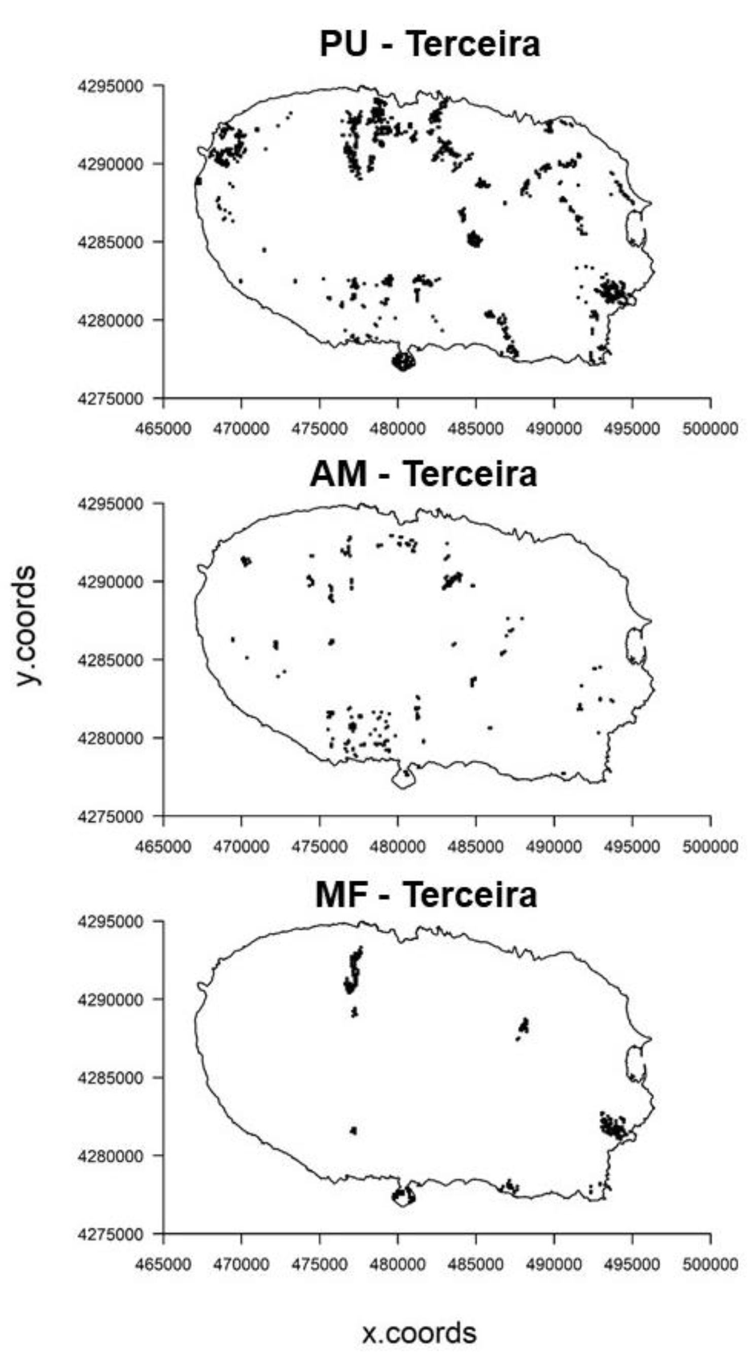
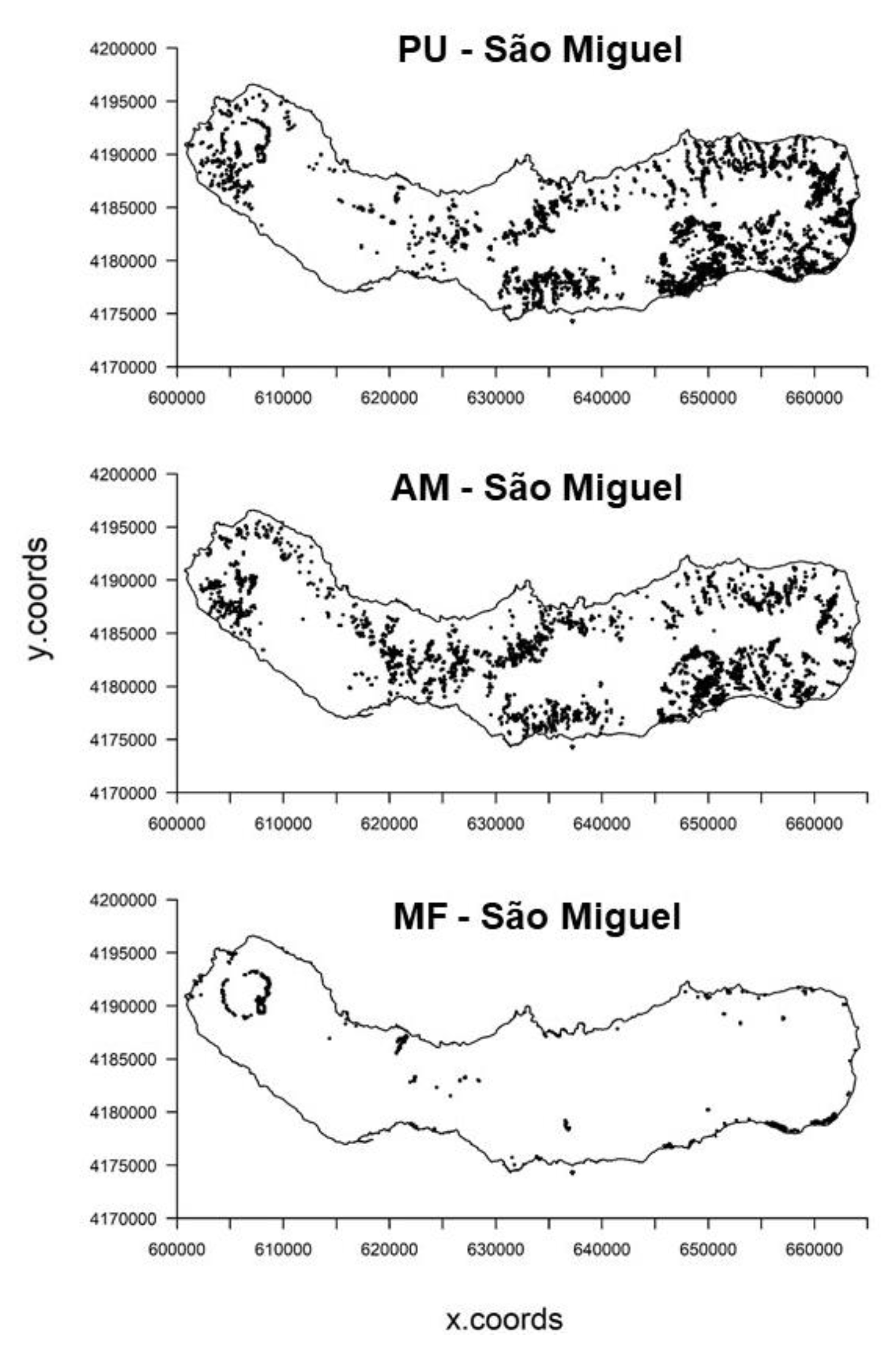
2.2.1. Species Data
2.2.2. Climate Data
2.2.3. Topographic Data
2.3. Modelling Approach
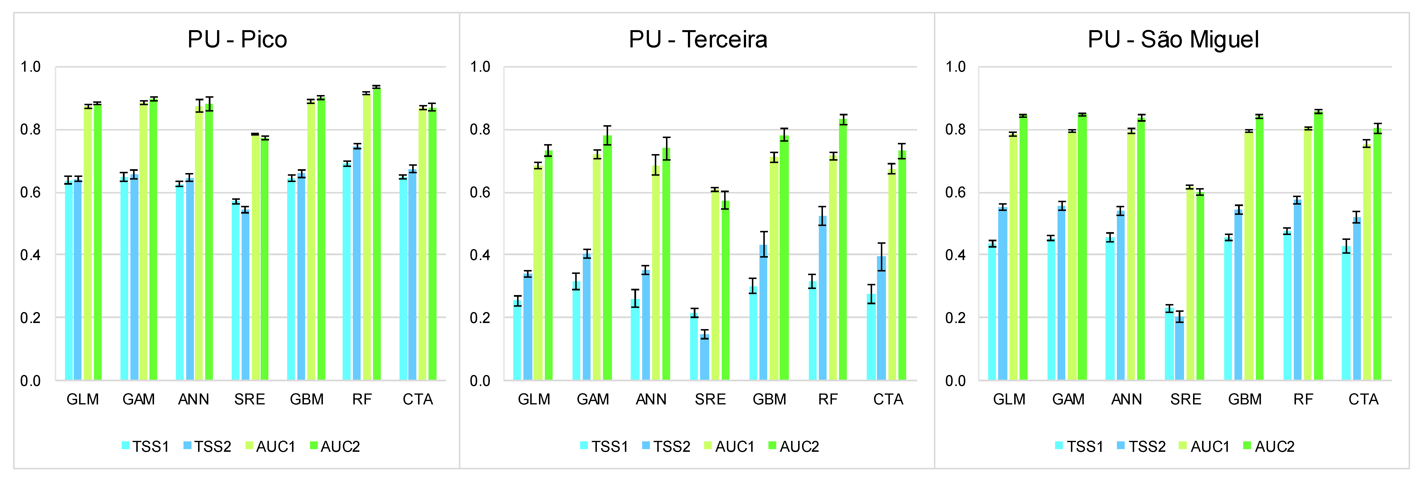
2.4. Model Validation
2.5. Model Projections
2.6. Variable Importance
3. Results
3.1. Summary of the Best Models
3.2. Relative Importance of EGVs
3.3. Present and Future Projections
4. Discussion
5. Conclusions
Supplementary Materials
Author Contributions
Funding
Acknowledgments
Conflicts of Interest
References
- Lackey, R.T. Seven pillars of ecosystem management. Landsc. Urban Plan. 1998, 40, 21–30. [Google Scholar] [CrossRef]
- Dukes, J.S.; Mooney, H.A. Does global change increase the success of biological invaders? Trends Ecol. Evol. 1999, 14, 135–139. [Google Scholar] [CrossRef]
- Landres, P.B.; Morgan, P.; Swanson, F.J. Overview of the use of natural variability concepts in managing ecological systems. Ecol. Appl. 1999, 9, 1179. [Google Scholar]
- Root, T.L.; Price, J.T.; Hall, K.R.; Schneider, S.H.; Rosenzweig, C.; Pounds, J.A. Fingerprints of global warming on wild animals and plants. Nature 2003, 421, 57–60. [Google Scholar] [CrossRef] [PubMed]
- Parmesan, C. Ecological and evolutionary responses to recent climate change. Annu. Rev. Ecol. Evol. Syst. 2006, 37, 637–669. [Google Scholar] [CrossRef]
- Lenoir, J.; Svenning, J.C. Climate-related range shifts: A global multidimensional synthesis and new research directions. Ecography 2015, 38, 15–28. [Google Scholar] [CrossRef]
- Walther, G.-R.; Roques, A.; Hulme, P.E.; Sykes, M.T.; Pysek, P.; Kühn, I.; Zobel, M.; Bacher, S.; Botta-Dukát, Z.; Bugmann, H.; et al. Alien species in a warmer world: Risks and opportunities. Trends Ecol. Evol. 2009, 24, 686–693. [Google Scholar] [CrossRef] [PubMed]
- Gallardo, B.; David, C.; Aldridge, D.C.; González-Moreno, P.; Jan Pergl, J.; Pizarro, M.; Pyšek, P.; Thuiller, W.; Yesson, C.; Vilà, M. Protected areas offer refuge from invasive species spreading under climate change. Glob. Change Biol. 2017, 23, 5331–5343. [Google Scholar] [CrossRef]
- Orians, G.H. An ecological and evolutionary approach to landscape aesthetics. In Landscape Meanings and Values; Penning-Rowsell, E.C., Lowenthal, D., Eds.; Allen and Unwin: London, UK, 1986; pp. 3–25. [Google Scholar]
- Peters, R.L.; Lovejoy, T.E. Global Warming and Biological Diversity; Yale University Press: Connecticut, NE, USA, 1992; p. 408. [Google Scholar]
- Vitousek, P.M.; D’Antonio, C.M.; Loope, L.L.; Westbrooks, R. Biological invasions as global environmental change. Am. Sci. 1996, 84, 468. [Google Scholar]
- Millar, C.I.; Stephenson, N.L.; Stephens, S.L. Climate change and forests of the future: Management in the face of uncertainty. Ecol. Appl. 2007, 17, 2145–2151. [Google Scholar] [CrossRef]
- Walther, G.-R.; Post, E.; Convey, P.; Menzel, A.; Parmesan, C.; Beebee, T.J.C.; Fromentin, J.-M.; Hoegh-Guldberg, O.; Bairlein, F. Ecological responses to recent climate change. Nature 2002, 416, 389–395. [Google Scholar] [CrossRef] [PubMed]
- Hellmann, J.J.; Byers, J.E.; Bierwagen, B.G.; Dukes, J.S. Five potential consequences of climate change for invasive species. Conserv. Biol. 2008, 22, 534–543. [Google Scholar] [CrossRef] [PubMed]
- Kerr, J.T.; Dobrowski, S.Z. Predicting the impacts of global change on species, communities and ecosystems: It takes time. Glob. Ecol. Biogeogr. 2013, 22, 261–263. [Google Scholar] [CrossRef]
- García, R.A.; Cabeza, M.; Rahbek, C.; Araújo, M.B. Multiple dimensions of climate change and their implications for biodiversity. Science 2014, 344, 1247579. [Google Scholar] [CrossRef] [PubMed]
- Mack, R.N.; Simberloff, D.; Lonsdale, W.M.; Evans, H.; Clout, M.; Bazzaz, F.A. Biotic invasions: Causes, epidemiology, global consequences, and control. Ecol. Appl. 2000, 10, 689–710. [Google Scholar] [CrossRef]
- Weltzin, J.F.; Bridgham, S.D.; Pastor, J.; Chen, J.; Harth, C. Potential effects of warming and drying on peatland plant community composition. Glob. Chang. Biol. 2003, 9, 141–151. [Google Scholar] [CrossRef]
- Thuiller, W. Biodiversity: Climate change and the ecologist. Nat. Reports Clim. Change 2007, 448, 60–62. [Google Scholar] [CrossRef]
- Thuiller, W.; Albert, C.; Araújo, M.B.; Berry, P.M.; Cabeza, M.; Guisan, A.; Hickler, T.; Midgley, G.F.; Paterson, J.; Schurr, F.M.; et al. Predicting global change impacts on plant species’ distributions: Future challenges. Perspect. Plant Ecol. Evol. Syst. 2008, 9, 137–152. [Google Scholar] [CrossRef]
- Bradley, B.A.; Oppenheimer, M.; Wilcove, D.S. Climate change and plant invasions: Restoration opportunities ahead? Glob. Chang. Biol. 2009, 15, 1511–1521. [Google Scholar] [CrossRef]
- Peters, R.L.; Darling, J.D.S. The greenhouse effect and nature reserves. Bioscience 1985, 35, 707–717. [Google Scholar] [CrossRef]
- Dudley, N. Forests and Climate Change; World Wildlife Fund International: Gland, Switzerland, 1998. [Google Scholar]
- Sala, O.E. Global biodiversity scenarios for the year 2100. Science 2000, 287, 1770–1774. [Google Scholar] [CrossRef] [PubMed]
- Noss, R.F. Beyond Kyoto: Forest management in a time of rapid climate change. Conserv. Biol. 2001, 15, 578–590. [Google Scholar] [CrossRef]
- Brooks, T.M.; Mittermeier, R.A.; Da Fonseca, G.A.B.; Gerlach, J.; Hoffmann, M.; Lamoreux, J.F.; Mittermeier, C.G.; Pilgrim, J.D.; Rodrigues, A.S.L.; Brooks, T. Global biodiversity conservation priorities. Science 2006, 313, 58–61. [Google Scholar] [CrossRef] [PubMed]
- Bush, A.A.; Nipperess, D.A.; Duursma, D.E.; Theischinger, G.; Turak, E.; Hughes, L. Continental-scale assessment of risk to the australian odonata from climate change. PLoS ONE 2014, 9, e88958. [Google Scholar] [CrossRef] [PubMed]
- Beerling, D.J. The impact of temperature on the northern distribution limits of the introduced species Fallopia japonica and Impatiens glandulifera in north-west Europe. J. Biogeogr. 1993, 20, 45. [Google Scholar] [CrossRef]
- Sutherst, R.W. The potential advance of pests in natural ecosystems under climate change: Implications for planning and management. Impacts of Climate Change on Ecosystems and Species: Terrestrial Ecosystems; IUCN: Gland, Switzerland, 1995; pp. 83–98. [Google Scholar]
- Zavaleta, E.S.; Royval, J.L. Climate change and the susceptibility of US ecosystems to biological invasions: Two cases of expected range expansion. In Wildlife Responses to Climate Change; Schneider, S.H., Root, T.L., Eds.; Island Press: Washington, DC, USA, 2002; pp. 277–341. [Google Scholar]
- Kriticos, D.; Sutherst, R.W.; Brown, J.R.; Adkins, S.W.; Maywald, G.F. Climate change and the potential distribution of an invasive alien plant: Acacia nilotica ssp. indica in Australia. J. Appl. Ecol. 2003, 40, 111–124. [Google Scholar] [CrossRef]
- Qian, H.; Ricklefs, R.E. The role of exotic species in homogenizing the North American flora. Ecol. Lett. 2006, 9, 1293–1298. [Google Scholar] [CrossRef]
- Mika, A.M.; Weiss, R.M.; Olfert, O.; Hallett, R.H.; Newman, J.A. Will climate change be beneficial or detrimental to the invasive swede midge in North America? Contrasting predictions using climate projections from different general circulation models. Glob. Chang. Biol. 2008, 14, 1721–1733. [Google Scholar] [CrossRef]
- Bradley, B.A.; Wilcove, D.S.; Oppenheimer, M. Climate change increases risk of plant invasion in the Eastern United States. Biol. Invasions 2010, 12, 1855–1872. [Google Scholar] [CrossRef]
- Vilà, M.; Vayreda, J.; Comas, L.; Ibáñez, J.J.; Mata, T.; Obon, B. Species richness and wood production: A positive association in Mediterranean forests. Ecol. Lett. 2007, 10, 241–250. [Google Scholar] [CrossRef]
- Weinberg, A.M. Science and trans-science. Minerva 1972, 10, 209–222. [Google Scholar] [CrossRef]
- Rastetter, E.B. Validating models of ecosystem response to global change. Bioscience 1996, 46, 190–198. [Google Scholar] [CrossRef]
- Thuiller, W.; Lavergne, S.; Roquet, C.; Boulangeat, I.; Lafourcade, B.; Araújo, M.B. Consequences of climate change on the tree of life in Europe. Nature 2011, 470, 531–534. [Google Scholar] [CrossRef] [PubMed]
- Lawler, J.J.; Ruesch, A.S.; Olden, J.; McRae, B.H. Projected climate-driven faunal movement routes. Ecol. Lett. 2013, 16, 1014–1022. [Google Scholar] [CrossRef] [PubMed]
- Casajus, N.; Périé, C.; Logan, T.; Lambert, M.-C.; De Blois, S.; Berteaux, D. An objective approach to select climate scenarios when projecting species distribution under climate change. PLoS ONE 2016, 11, e0152495. [Google Scholar] [CrossRef] [PubMed]
- Clavero, M.; Villero, D.; Brotons, L. Climate change or land use dynamics: Do we know what climate change indicators indicate? PLoS ONE 2011, 6, e18581. [Google Scholar] [CrossRef] [PubMed]
- Barnagaud, J.-Y.; Devictor, V.; Jiguet, F.; Barbet-Massin, M.; Le Viol, I.; Archaux, F. Relating habitat and climatic niches in birds. PLoS ONE 2012, 7, e32819. [Google Scholar] [CrossRef] [PubMed]
- Barnagaud, J.-Y.; Barbaro, L.; Hampe, A.; Jiguet, F.; Archaux, F. Species’ thermal preferences affect forest bird communities along landscape and local scale habitat gradients. Ecography 2013, 36, 1218–1226. [Google Scholar] [CrossRef]
- Schaefer, K.; Schuur, E.A.G.; Witt, R.; Lantuit, H.; E Romanovsky, V. The impact of the permafrost carbon feedback on global climate. Environ. Res. Lett. 2014, 9, 085003. [Google Scholar] [CrossRef]
- Regos, A.; Clavero, M.; D’amen, M.; Guisan, A.; Brotons, L. Wildfire-vegetation dynamics affect predictions of climate change impact on bird communities. Ecography 2018, 41, 982–995. [Google Scholar] [CrossRef]
- Elith, J.; Graham, C.H.; Anderson, R.P.; Dudík, M.; Ferrier, S.; Guisan, A.; Hijmans, R.J.; Huettmann, F.; Leathwick, J.R.; Lehmann, A.; et al. Novel methods improve prediction of species’ distributions from occurrence data. Ecography 2006, 29, 129–151. [Google Scholar] [CrossRef]
- Guisan, A.; Thuiller, W. Predicting species distribution: Offering more than simple habitat models. Ecol. Lett. 2005, 8, 993–1009. [Google Scholar] [CrossRef]
- Elith, J.; Leathwick, J.R. Species distribution models: Ecological explanation and prediction across space and time. Annu. Rev. Ecol. Evol. Syst. 2009, 40, 677–697. [Google Scholar] [CrossRef]
- Bellard, C.; Leclerc, C.; Courchamp, F. Impact of sea level rise on the 10 insular biodiversity hotspots. Glob. Ecol. Biogeogr. 2014, 23, 203–212. [Google Scholar] [CrossRef]
- Steadman, D.W. Extinction and Biogeography of Tropical Pacific Birds; University of Chicago Press: Chicago, IL, USA, 2006; p. 480. [Google Scholar]
- Whittaker, R.J.; Fernández-Palacios, J.M. Island Biogeography: Ecology, Evolution, and Conservation, 2nd ed.; Oxford University Press: Oxford, UK, 2007; p. 416. [Google Scholar]
- Triantis, K.A.; Borges, P.A.V.; Ladle, R.J.; Hortal, J.; Cardoso, P.; Gaspar, C.; Dinis, F.; Mendonça, E.; Silveira, L.M.A.; Gabriel, R.; et al. Extinction debt on oceanic islands. Ecography 2010, 33, 285–294. [Google Scholar] [CrossRef]
- Silva, L.; Dias, E.F.; Sardos, J.; Azevedo, E.B.; Schaefer, H.; Moura, M.; Azevedo, E.B. Towards a more holistic research approach to plant conservation: The case of rare plants on oceanic islands. AoB PLANTS 2015, 7, 066. [Google Scholar] [CrossRef] [PubMed]
- Paulay, G. Biodiversity on oceanic islands: Its origin and extinction 1. Am. Zool. 1994, 34, 134–144. [Google Scholar] [CrossRef]
- Thompson, K.; Hodgson, J.G.; Rich, T.C.G. Native and alien invasive plants: More of the same? Ecography 1995, 18, 390–402. [Google Scholar] [CrossRef]
- Blackburn, T.M.; Cassey, P.; Duncan, R.P.; Evans, K.L.; Gaston, K.J. Avian extinction and mammalian introductions on oceanic islands. Science 2004, 305, 1955–1958. [Google Scholar] [CrossRef]
- Sax, D.F.; Gaines, S.D. Species invasions and extinction: The future of native biodiversity on islands. Proc. Natl. Acad. Sci. USA 2008, 105, 11490–11497. [Google Scholar] [CrossRef]
- Raposeiro, P.M.; Rubio, M.J.; González, A.; Hernández, A.; Sánchez-López, G.; Vázquez-Loureiro, D.; Rull, V.; Bao, R.; Costa, A.C.; Gonçalves, V.; et al. Impact of the historical introduction of exotic fishes on the chironomid community of Lake Azul (Azores Islands). Palaeogeogr. Palaeoclim. Palaeoecol. 2017, 466, 77–88. [Google Scholar] [CrossRef]
- Cowie, R.H.; Holland, B.S. Dispersal is fundamental to biogeography and the evolution of biodiversity on oceanic islands. J. Biogeogr. 2006, 33, 193–198. [Google Scholar] [CrossRef]
- Sadler, J.P. Biodiversity on oceanic islands: A palaeoecological assessment. J. Biogeogr. 1999, 26, 75–87. [Google Scholar] [CrossRef]
- Markham, A. Potential impacts of climate change on tropical forest ecosystems. Clim. Chang. 1998, 39, 141–143. [Google Scholar] [CrossRef]
- Ferreira, M.T.; Cardoso, P.; Borges, P.A.; Gabriel, R.; Azevedo, E.B.; Reis, F.; Araújo, M.B.; Elias, R.B. Effects of climate change on the distribution of indigenous species in oceanic islands (Azores). Clim. Chang. 2016, 138, 603–615. [Google Scholar] [CrossRef]
- Santos, F.D.; Valente, M.A.; Miranda, P.M.A.; Aguiar, A.; Azevedo, E.B.; Tomé, A.R.; Coelho, F. Climate change scenarios in the Azores and Madeira islands. World Resource Rev. 2004, 16, 473–491. [Google Scholar]
- Thomas, C.D.; Cameron, A.; Green, R.E.; Bakkenes, M.; Beaumont, L.J.; Collingham, Y.C.; Erasmus, B.F.N.; De Siqueira, M.F.; Grainger, A.; Hannah, L.; et al. Extinction risk from climate change. Nature 2004, 427, 145–148. [Google Scholar] [CrossRef]
- Thom, D.; Rammer, W.; Dirnböck, T.; Müller, J.; Kobler, J.; Katzensteiner, K.; Helm, N.; Seidl, R. The impacts of climate change and disturbance on spatio-temporal trajectories of biodiversity in a temperate forest landscape. J. Appl. Ecol. 2017, 54, 28–38. [Google Scholar] [CrossRef]
- Myers, N.; Mittermeier, R.A.; Mittermeier, C.G.; Da Fonseca, G.A.B.; Kent, J. Biodiversity hotspots for conservation priorities. Nature 2000, 403, 853–858. [Google Scholar] [CrossRef]
- Parrotta, J.A.; Wildburger, C.; Mansourian, S. Understanding relationships between biodiversity, carbon, forests and people: The key to achieving REDD+ objectives. IUFRO World Series (Austria) 2012, eng v. 31. Available online: https://www.fs.usda.gov/treesearch/pubs/download/47822.pdf (accessed on 21 November 2017).
- Bourque, C.-A.; Hassan, Q.K.; Swift, D.E. Modelled potential species distribution for current and projected future climates for the Acadian Forest region of Nova Scotia, Canada. Report prepared for the Nova Scotia Department of Natural Resources, Truro, Nova Scotia; 2008; p. 46. Available online: http://www.gov.ns.ca/natr/forestry/reports/Final-Report-for-NS-Climate-Change Project (accessed on 12 October 2017).
- Silva, L.; Smith, C.W. A quantitative approach to the study of non-indigenous plants: An example from the Azores Archipelago. Biodivers. Conserv. 2006, 15, 1661–1679. [Google Scholar] [CrossRef]
- Silva, L.; Ojeda-Land, E.; Rodríguez-Luengo, J.L. Invasive Terrestrial Flora and Fauna of Macaronesia. Top 100 in Azores, Madeira and Canaries; ARENA: Ponta Delgada, Portugal, 2008; pp. 167–188. [Google Scholar]
- Costa, H.; Aranda, S.C.; Lourenço, P.; Medeiros, V.; Azevedo, E.B.; Silva, L. Predicting successful replacement of forest invaders by native species using species distribution models: The case of Pittosporum undulatum and Morella faya in the Azores. For. Ecol. Manag. 2012, 279, 90–96. [Google Scholar] [CrossRef]
- Hortal, J.; Borges, P.A.; Jiménez-Valverde, A.; Azevedo, E.B.; Silva, L. Assessing the areas under risk of invasion within islands through potential distribution modelling: The case of Pittosporum undulatum in São Miguel, Azores. J. Nat. Conserv. 2010, 18, 247–257. [Google Scholar] [CrossRef]
- Thuiller, W. BIOMOD—Optimizing predictions of species distributions and projecting potential future shifts under global change. Glob. Chang. Boil. 2003, 9, 1353–1362. [Google Scholar] [CrossRef]
- Costa, H.; Medeiros, V.; Azevedo, E.B.; Silva, L. Evaluating ecological-niche factor analysis as a modelling tool for environmental weed management in island systems. Weed Res. 2013, 53, 221–230. [Google Scholar] [CrossRef]
- Costa, H.; Ponte, N.B.; Azevedo, E.B.; Gil, A. Fuzzy set theory for predicting the potential distribution and cost-effective monitoring of invasive species. Ecol. Model. 2015, 316, 122–132. [Google Scholar] [CrossRef]
- Borges, P.A.V.; Lobo, J.M.; Azevedo, E.B.; Gaspar, C.S.; Melo, C.; Nunes, L.V. Invasibility and species richness of island endemic arthropods: A general model of endemic vs. exotic species. J. Biogeogr. 2006, 33, 169–187. [Google Scholar] [CrossRef]
- Gabriel, R.; Coelho, M.M.C.; Henriques, D.S.G.; Borges, P.A.V.; Elias, R.B.; Kluge, J.; Ah-Peng, C. Long-term monitoring across elevational gradients to assess ecological hypothesis: A description of standardized sampling methods in oceanic islands and first results. Arquipelago. Life Mar. Sci. 2014, 31, 45–67. [Google Scholar]
- Elias, R.B.; Gil, A.; Silva, L.; Fernández-Palacios, J.M.; Azevedo, E.B.; Reis, F. Natural zonal vegetation of the Azores Islands: Characterization and potential distribution. Phytocoenologia 2016, 46, 107–123. [Google Scholar] [CrossRef]
- Silveira, L.M.A. Learning with History: Interaction with Nature during the Human Colonization in Terceira Island. Dissertation. Master Degree, University of Azores, Angra do Heroísmo, 2007. [Google Scholar]
- Gaspar, C.; Borges, P.A.; Gaston, K.J. Diversity and distribution of arthropods in native forests of the Azores archipelago. 2008. Available online: http://hdl.handle.net/10400.3/249 (accessed on 17 July 2017).
- Borges Silva, L.; Lourenço, P.; Ponte, N.B.; Medeiros, V.; Elias, R.B.; Alves, M.; Silva, L.; Pinto, A.A.; Zilberman, D. Development of Allometric Equations for Estimating Above-Ground Biomass of Woody Plant Invaders: The Case of Pittosporum undulatum in the Azores Archipelago. In Intelligent Techniques in Engineering Management; Springer Science and Business Media LLC.: Berlin, Germany, 2017; Volume 195, pp. 463–484. [Google Scholar]
- Borges Silva, L.; Lourenco, P.; Teixeira, A.; Azevedo, E.; Alves, M.; Elias, R.; Silva, L. Biomass valorization in the management of woody plant invaders: The case of Pittosporum undulatum in the Azores. Biomass Bioenergy 2018, 109, 155–165. [Google Scholar] [CrossRef]
- Direcção Regional dos Recursos Florestais (DRRF). Avaliação da Biomassa Disponível em Povoamentos Florestais na Região Autónoma dos Açores. Inventário Florestal da Região Autónoma dos Açores; Direcção Regional dos Recursos Florestais, Secretaria Regional da Agricultura e Florestas da Região Autónoma dos Açores: Ponta Delgada, Portugal, 2007; p. 8. [Google Scholar]
- Gleadow, R.M.; Ashton, D.H. Invasion by Pittosporum undulatum of the forests of central Victoria. I. Invasion patterns and plant morphology. Aust. J. Bot. 1981, 29, 705–720. [Google Scholar] [CrossRef]
- Harden, G.J. Flora of New South Wales; New South Wales University Press: Kensington, UK, 1992; Volume 3. [Google Scholar]
- Bellingham, P.J.; Tanner, E.V.; Healey, J.R. Hurricane disturbance accelerates invasion by the alien tree Pittosporum undulatum in Jamaican montane rain forests. J. Veg. Sci. 2005, 16, 675–684. [Google Scholar] [CrossRef]
- Dias, E.; Aráujo, C.; Mendes, J.F.; Elias, R.B.; Mendes, C.; Melo, C. Espécies florestais das ilhas Açores. In Árvores e florestas de Portugal; Público, Comunicação Social; SA/Fundação Luso-Americana/Liga para a Protecção da Natureza: Lisboa, Portugal, 2007; Volume 6, pp. 199–254. ISBN 978-989-619-103-0. [Google Scholar]
- Ferreira, N.J.; Meireles de Sousa, I.G.; Luís, T.C.; Currais, A.J.M.; Figueiredo, A.C.; Costa, M.M.; Lima, A.S.B.; Santos, P.A.G.; Barroso, J.G.; Pedro, L.G.; et al. Pittosporum undulatum Vent. grown in Portugal: Secretory structures, seasonal variation and enantiomeric composition of its essential oil. Flavour Frag. J. 2007, 22, 1–9. [Google Scholar] [CrossRef]
- Cronk, Q.C.B.; Fuller, J.L. Plant Invaders: The threat to natural ecosystems; Chapman and Hall: New York, NY, USA, 2014; p. 241. [Google Scholar]
- Lourenço, P.; Medeiros, V.; Gil, A.; Silva, L. Distribution, habitat and biomass of Pittosporum undulatum, the most important woody plant invader in the Azores Archipelago. For. Ecol. Manag. 2011, 262, 178–187. [Google Scholar] [CrossRef]
- Dutra Silva, L.; Costa, H.; Azevedo, E.B.; Medeiros, V.; Alves, M.; Elias, R.B.; Silva, L.; Pinto, A.A.; Zilberman, D. Modelling Native and Invasive Woody Species: A Comparison of ENFA and MaxEnt Applied to the Azorean Forest. In Intelligent Techniques in Engineering Management; Springer Science and Business Media LLC.: Berlin, Germany, 2017; Volume 195, pp. 415–444. [Google Scholar]
- Dutra Silva, L.; Azevedo, E.B.; Elias, R.B.; Silva, L. Species distribution modeling: Comparison of fixed and mixed effects models using INLA. ISPRS Int. J. Geo-Information 2017, 6, 391. [Google Scholar] [CrossRef]
- Sjögren, E. Recent changes in the vascular flora and vegetation of the Azores Islands. Memórias da Sociedade Broteriana 1973, 22, 1–113. [Google Scholar]
- Silva, L.; Tavares, J. Phytophagous Insects Associated with Endemic, Macaronesian, and Exotic Plants in the Azores. In Avances en Entomologia Ibérica; Museo Nacional de Ciencias Naturales (CSIC) y Universidad Autónoma de Madrid: Madrid, Spain, 1995; pp. 179–187. [Google Scholar]
- Wagner, W.L.; Herbst, D.R.; Sohmer, S.H. Manual of the Flowering Plants of Hawai’i, 2nd ed.; University of Hawai’i and Bishop Museum Press: Honolulu, HI, USA, 1999; Volumes 1 and 2, p. 1952. [Google Scholar]
- Dröuet, H. Catalogue de la Flore des îles Açores; Baillière and Fils: Paris, France, 1866. [Google Scholar]
- Silva, L.; Tavares, J. Factors affecting Myrica faya Aiton demography in the Azores. Açoreana 1997, 8, 359–374. [Google Scholar]
- Azevedo, E.B. Modelação do Clima Insular à Escala Local. Modelo CIELO aplicado à ilha Terceira; Dissertation, PhD, Universidade dos Açores: Angra do Heroísmo, Portugal, 1996. [Google Scholar]
- Azevedo, E.B.; Pereira, L.S.; Itier, B. Modelling the local climate in island environments: Water balance applications. Agric. Water Manag. 1999, 40, 393–403. [Google Scholar] [CrossRef]
- Azevedo, E.B. Projecto CLIMAAT - Clima e Meteorologia dos Arquipélagos Atlânticos, PIC Interreg IIIB Mac2, 3/A3; Universidade dos Açores: Angra do Heroísmo, Portugal, 2003; Unpublished report on file. [Google Scholar]
- IPCC-AR5. Summary for Policymakers. In Climate Change 2014: Mitigation of Climate Change; Contribution of Working Group III to the Fifth Assessment Report of the Intergovernmental Panel on Climate Change; Edenhofer, O., Pichs-Madruga, R., Sokona, Y., Farahani, E., Kadner, S., Seyboth, K., Adler, A., Baum, I., Brunner, S., Eickemeier, P., et al., Eds.; Cambridge University Press: Cambridge, UK, 2014. [Google Scholar]
- Peters, G.P.; Andrew, R.M.; Boden, T.; Canadell, J.G.; Ciais, P.; Le Quéré, C.; Marland, G.; Raupach, M.R.; Wilson, C. The challenge to keep global warming below 2 °C. Nat. Clim. Chang. 2013, 3, 4. [Google Scholar] [CrossRef]
- Araújo, M.B.; New, M. Ensemble forecasting of species distributions. Trends Ecol. Evol. 2007, 22, 42–47. [Google Scholar] [CrossRef]
- Thuiller, W.; Lafourcade, B.; Engler, R.; Araújo, M.B. BIOMOD – a platform for ensemble forecasting of species distributions. Ecography 2009, 32, 369–373. [Google Scholar] [CrossRef]
- Thuiller, W.; Georges, D.; Engler, R.; Breiner, F.; Georges, M.D.; Thuiller, C.W. Package ‘biomod2′. Version 3.3-7. Available online: https://cran.r-project.org/web/packages/biomod2/biomod2.pdf (accessed on 15 May 2019).
- R Development Core Team. R: A Language and Environment for Statistical Computing; R Foundation for Statistical Computing: Vienna, Austria, 2016; Available online: www.R-project.org (accessed on 12 June 2017).
- McCullagh, P.; Nelder, J.A. Generalized Linear Models no. 37 in Monograph on Statistics and Applied Probability; Chapman & Hall: London, UK, 1989; p. 532. [Google Scholar]
- Hastie, T.J. Tibshirani R.J. Generalized Additive Models; CRC Press: Boca Raton, FL, USA, 1990; p. 352. [Google Scholar]
- Venables, W.N.; Ripley, B.D. Random and mixed effects. In Modern Applied Statistics with S.; Springer: New York, NY, USA, 2002; pp. 271–300. [Google Scholar]
- Ripley, B.D. Pattern Recognition and Neural Networks; Cambridge University Press: London, UK, 2007; p. 416. [Google Scholar]
- White, H. Learning in artificial neural networks: A statistical perspective. Learning 2008, 1. [Google Scholar] [CrossRef]
- Ridgeway, G. The state of boosting. Comput. Sci. Stat. 1999, 31, 172–181. [Google Scholar]
- Breiman, L. Random forests. Mach. Learn. 2001, 45, 5–32. [Google Scholar] [CrossRef]
- Gordon, A.D.; Breiman, L.; Friedman, J.H.; Olshen, R.A.; Stone, C.J. Classification and Regression Trees. Biological 1984, 40, 874. [Google Scholar] [CrossRef]
- Busby, J. BIOCLIM –a bioclimate analysis and prediction system. Plant Prot. Q. (Aust.) 1991, 6, 8–9. [Google Scholar]
- Dobson, A.J.; Barnett, A. An Introduction to Generalized Linear Models; CRC Press: Boca Raton, FL, USA, 2008; p. 320. [Google Scholar]
- Singer, A.; Millat, G.; Staneva, J.; Kröncke, I. Modelling benthic macrofauna and seagrass distribution patterns in a North Sea tidal basin in response to 2050 climatic and environmental scenarios. Estuarine, Coast. Shelf Sci. 2017, 188, 99–108. [Google Scholar] [CrossRef]
- Rigby, R.A.; Stasinopoulos, D.M. Generalized additive models for location, scale and shape. SJ. R. Stat. Soc. er. C. 2005, 54, 507–554. [Google Scholar] [CrossRef]
- Haykin, S. Neural Networks a Comprehensive Introduction; Prentice Hall PTR: Upper Saddle River, NJ, USA, 1999; p. 938. [Google Scholar]
- Park, Y.-S.; Céréghino, R.; Compin, A.; Lek, S. Applications of artificial neural networks for patterning and predicting aquatic insect species richness in running waters. Ecol. Model. 2003, 160, 265–280. [Google Scholar] [CrossRef]
- Svetnik, V.; Liaw, A.; Tong, C.; Culberson, J.C.; Sheridan, R.P.; Feuston, B.P. Random Forest: A classification and regression tool for compound classification and QSAR modeling. J. Chem. Inf. Comput. Sci. 2003, 43, 1947–1958. [Google Scholar] [CrossRef]
- Prasad, A.M.; Iverson, L.R.; Liaw, A. Newer classification and regression tree techniques: Bagging and Random Forests for ecological prediction. Ecosystems 2006, 9, 181–199. [Google Scholar] [CrossRef]
- Lawrence, R.L.; Ripple, W.J. Fifteen years of revegetation of Mount St. Helens: A landscape-scale analysis. Ecology 2000, 81, 2742–2752. [Google Scholar] [CrossRef]
- Lawrence, R.; Bunn, A.; Powell, S.; Zambon, M. Classification of remotely sensed imagery using stochastic gradient boosting as a refinement of classification tree analysis. Remote. Sens. Environ. 2004, 90, 331–336. [Google Scholar] [CrossRef]
- Nix, H.A.; Busby, J. BIOCLIM, a Bioclimatic Analysis and Prediction System; Division of Water and Land Resources: Canberra, Australia, 1986. [Google Scholar]
- Lomba, Â.; Pellissier, L.; Randin, C.; Vicente, J.; Moreira, F.; Honrado, J.; Guisan, A. Overcoming the rare species modelling paradox: A novel hierarchical framework applied to an Iberian endemic plant. Biol. Conserv. 2010, 143, 2647–2657. [Google Scholar] [CrossRef]
- Mayer, K.; Haeuser, E.; Dawson, W.; Essl, F.; Kreft, H.; Pergl, J.; Pyšek, P.; Weigelt, P.; Lenzner, B.; Winter, M.; et al. Naturalization of ornamental plant species in public green spaces and private gardens. Biol. Invasions 2017, 19, 3613–3627. [Google Scholar] [CrossRef]
- Merow, C.; Smith, M.J.; Edwards, T.C., Jr.; Guisan, A.; McMahon, S.M.; Normand, S.; Wilfried Thuiller, W.; Wüest, R.O.; Zimmermann, N.E.; Elith, J. What do we gain from simplicity versus complexity in species distribution models? Ecography 2014, 37, 1267–1281. [Google Scholar] [CrossRef]
- Barbet-Massin, M.; Jiguet, F.; Albert, C.H.; Thuiller, W.; Barbet-Massin, M. Selecting pseudo-absences for species distribution models: How, where and how many? Methods Ecol. Evol. 2012, 3, 327–338. [Google Scholar] [CrossRef]
- Hijmans, R.J.; van Etten, J.; Cheng, J.; Mattiuzzi, M.; Sumner, M.; Greenberg, J.A.; Lamigueiro, O.P.; Bevan, A.; Racine, E.B.; Shortridge, A. Package ‘raster’. R package 2016. Available online: https://cran.r-project.org/web/packages/raster/index.html (accessed on 2 September 2017).
- Quillfeldt, P.; Engler, J.O.; Silk, J.R.; Phillips, R.A. Influence of device accuracy and choice of algorithm for species distribution modelling of seabirds: A case study using black-browed albatrosses. J. Avian Boil. 2017, 48, 1549–1555. [Google Scholar] [CrossRef]
- Allouche, O.; Tsoar, A.; Kadmon, R. Assessing the accuracy of species distribution models: Prevalence, kappa and the true skill statistic (TSS). J. Appl. Ecol. 2006, 43, 1223–1232. [Google Scholar] [CrossRef]
- Fielding, A.H.; Bell, J.F. A review of methods for the assessment of prediction errors in conservation presence/absence models. Environ. Conserv. 1997, 24, 38–49. [Google Scholar] [CrossRef]
- Pearson, R.G. Species’ distribution modeling for conservation educators and practitioners. Available online: https://pdfs.semanticscholar.org/66db/947ee1a6ab91c408f489d17cfb6e068931a6.pdf (accessed on 22 May 2017).
- Landis, J.R.; Koch, G.G. An application of hierarchical Kappa-type statistics in the assessment of majority agreement among multiple observers. Biometrics 1977, 33, 363. [Google Scholar] [CrossRef]
- Coetzee, B.W.T.; Robertson, M.P.; Erasmus, B.F.N.; Van Rensburg, B.J.; Thuiller, W. Ensemble models predict Important bird areas in southern Africa will become less effective for conserving endemic birds under climate change. Glob. Ecol. Biogeogr. 2009, 18, 701–710. [Google Scholar] [CrossRef]
- Peterson, A.T.; Papeş, M.; Soberón, J. Rethinking receiver operating characteristic analysis applications in ecological niche modeling. Ecol. Model. 2008, 213, 63–72. [Google Scholar] [CrossRef]
- Hernandez, P.A.; Graham, C.H.; Master, L.L.; Albert, D.L. The effect of sample size and species characteristics on performance of different species distribution modeling methods. Ecography 2006, 29, 773–785. [Google Scholar] [CrossRef]
- Swets, J. Measuring the accuracy of diagnostic systems. Science 1988, 240, 1285–1293. [Google Scholar] [CrossRef] [PubMed]
- Bellard, C.; Bertelsmeier, C.; Leadley, P.; Thuiller, W.; Courchamp, F. Impacts of climate change on the future of biodiversity. Ecol. Lett. 2012, 15, 365–377. [Google Scholar] [CrossRef] [PubMed]
- Solomon, S. Climate Change 2007—The Physical Science Basis: Working Group I Contribution to the Fourth Assessment Report of the IPCC; Cambridge University Press: London, UK.
- Thuiller, W.; Brotons, L.; Araújo, M.B.; Lavorel, S. Effects of restricting environmental range of data to project current and future species distributions. Ecography 2004, 27, 165–172. [Google Scholar] [CrossRef]
- Araújo, M.B.; Whittaker, R.J.; Ladle, R.J.; Erhard, M. Reducing uncertainty in projections of extinction risk from climate change. Glob. Ecol. Biogeogr. 2005, 14, 529–538. [Google Scholar] [CrossRef]
- Gama, M.; Crespo, D.; Dolbeth, M.; Anastacio, P. Predicting global habitat suitability for Corbicula fluminea using species distribution models: The importance of different environmental datasets. Ecol. Model. 2016, 319, 163–169. [Google Scholar] [CrossRef]
- Araújo, M.B.; Cabeza, M.; Thuiller, W.; Hannah, L.; Williams, P.H. Would climate change drive species out of reserves? An assessment of existing reserve-selection methods. Glob. Chang. Biol. 2004, 10, 1618–1626. [Google Scholar] [CrossRef]
- Lawton, J.H. Range, population abundance and conservation. Trends Ecol. Evol. 1993, 8, 409–413. [Google Scholar] [CrossRef]
- Pimm, S.L. Community stability and structure. In Conservation Biology: The Science of Scarcity and Diversity; Soule’, M., Ed.; Simauer: Sunderland, MA, USA, 1996; pp. 309–329. [Google Scholar]
- Hirzel, A.H.; Perrin, N.; Hausser, J.; Chessel, D. Ecological-niche factor analysis: How to compute habitat-suitability maps without absence data? Ecology 2002, 83, 2027–2036. [Google Scholar] [CrossRef]
- Hirzel, A.H.; Le Lay, G.; Helfer, V.; Randin, C.; Guisan, A. Evaluating the ability of habitat suitability models to predict species presences. Ecol. Model. 2006, 199, 142–152. [Google Scholar] [CrossRef]
- Caruana, R.; Karampatziakis, N.; Yessenalina, A. An empirical evaluation of supervised learning in high dimensions. In Proceedings of the 25th International Conference on Machine Learning, Helsinki, Finland, 5–9 July 2008; pp. 96–103. [Google Scholar]
- Scales, K.L.; Miller, P.I.; Ingram, S.N.; Hazen, E.L.; Bograd, S.J.; Phillips, R.A. Identifying predictable foraging habitats for a wide-ranging marine predator using ensemble ecological niche models. Divers. Distrib. 2016, 22, 212–224. [Google Scholar] [CrossRef]
- Dullinger, I.; Wessely, J.; Bossdorf, O.; Dawson, W.; Essl, F.; Gattringer, A.; Klonner, G.; Kreft, H.; Kuttner, M.; Moser, D.; et al. Climate change will increase the naturalization risk from garden plants in Europe. Glob. Ecol. Biogeogr. 2017, 26(1), 43–53. [Google Scholar] [CrossRef]
- Oppel, S.; Meirinho, A.; Ramírez, I.; Gardner, B.; O’Connell, A.F.; Miller, P.I.; Louzao, M. Comparison of five modelling techniques to predict the spatial distribution and abundance of seabirds. Biol. Conserv. 2012, 156, 94–104. [Google Scholar] [CrossRef]
- Segurado, P.; Araújo, M.B. An evaluation of methods for modelling species distributions. J. Biogeogr. 2004, 31, 1555–1568. [Google Scholar] [CrossRef]
- Syphard, A.D.; Franklin, J. Differences in spatial predictions among species distribution modeling methods vary with species traits and environmental predictors. Ecography 2009, 32, 907–918. [Google Scholar] [CrossRef]
- Hauenstein, S.; Wood, S.N.; Dormann, C.F. Computing AIC for black-box models using generalized degrees of freedom: A comparison with cross-validation. Commun. Stat. Simul. Comput. 2018, 47, 1382–1396. [Google Scholar] [CrossRef]
- Lobo, J.M.; Real, R.; Jiménez-Valverde, A.; Jiménez-Valverde, A. AUC: A misleading measure of the performance of predictive distribution models. Glob. Ecol. Biogeogr. 2008, 17, 145–151. [Google Scholar] [CrossRef]
- Jimenez-Valverde, A.; Peterson, A.T.; Soberon, J.; Overton, J.M.; Aragón, P.; Lobo, J.M. Use of niche models in invasive species risk assessments. Biol. Invasions 2011, 13, 2785–2797. [Google Scholar] [CrossRef]
- Wisz, M.S.; Pottier, J.; Kissling., D.; Pellissier, L.; Lenoir, J.; Damgaards, C.F.; Dormann, C.F.; Forchhammer, M.C.; Grytnes, J.; Guisan, A.; et al. The role of biotic interactions in shaping distributions and realised assemblages of species: Implications for species distribution modelling. Biol. Rev. 2013, 88, 15–30. [Google Scholar] [CrossRef] [PubMed]
- Skov, F.; Svenning, J.-C.; Svenning, J.-C.; Svenning, J. Could the tree diversity pattern in Europe be generated by postglacial dispersal limitation? Ecol. Lett. 2007, 10, 453–460. [Google Scholar]
- Valladares, F.; Matesanz, S.; Guilhaumon, F.; Araújo, M.B.; Balaguer, L.; Benito-Garzón, M.; Cornwell, W.; Gianoli, E.; Van Kleunen, M.; Naya, D.E.; et al. The effects of phenotypic plasticity and local adaptation on forecasts of species range shifts under climate change. Ecol. Lett. 2014, 17, 1351–1364. [Google Scholar] [CrossRef] [PubMed]
- Sitzia, T.; Campagnaro, T.; Kowarik, I.; Trentanovi, G. Using forest management to control invasive alien species: Helping implement the new European regulation on invasive alien species. Biol. Invasions. 2016, 18, 1–7. [Google Scholar] [CrossRef]
- PRAC. Programa Regional para as Alterações Climáticas dos Açores. Available online: www.azores.gov.pt/Gra/srrn-ambiente/menus/secundario/PRAC/. (accessed on 3 November 2017).
- Azevedo, E.B.; Reis, F.V. PRoAAcXXIs - Projeções das Alterações Climática nos Açores para o século XXI - Implicações Hidrológicas de interesse Agronómico e Ambiental – 1º Relatório de Progresso; University of the Azores: Angra do Heroísmo, Portugal, 2017; p. 23. [Google Scholar]


| Environmental Variables | Code | Units | Data Type | Data Source |
|---|---|---|---|---|
| Annual minimum temperature | TMIN | °C | Climatic | CIELO model 1,2 |
| Annual maximum temperature | TMAX | |||
| Annual mean temperature | TM | |||
| Annual minimum relative humidity | RHMIN | % | ||
| Annual maximum relative humidity | RHMAX | |||
| Total annual precipitation | PT | mm | ||
| Elevation | DEM | m | Topographical | CIELO model DEM |
| Aspect | ASP | ° | ||
| Slope | SLP | % | ||
| Curvature | CRV | |||
| Flow accumulation | FLA | |||
| Summer hill shade | SHS | |||
| Winter hill shade | WHS |
| Variables | Pico Island | Terceira Island | São Miguel Island | |||||||||||||||
|---|---|---|---|---|---|---|---|---|---|---|---|---|---|---|---|---|---|---|
| Min. | Q1 | Median | Mean | Q3 | Max. | Min. | Q1 | Median | Mean | Q3 | Max. | Min. | Q1 | Median | Mean | Q3 | Max. | |
| Present | ||||||||||||||||||
| TMIN | 1.1 | 10.8 | 12.7 | 12.6 | 14.7 | 17.6 | 7.8 | 11.5 | 12.6 | 12.6 | 14.0 | 15.6 | 6.6 | 10.8 | 12.2 | 12.0 | 13.3 | 15.7 |
| TMAX | 7.4 | 16.1 | 17.9 | 17.9 | 19.8 | 22.9 | 13.5 | 16.9 | 18.0 | 18.0 | 19.3 | 20.9 | 13.3 | 17.3 | 18.6 | 18.4 | 19.7 | 22.2 |
| TM | 4.3 | 13.5 | 15.3 | 15.2 | 17.2 | 20.2 | 10.7 | 14.2 | 15.3 | 15.3 | 16.7 | 18.2 | 10.0 | 14.0 | 15.4 | 15.2 | 16.5 | 18.9 |
| RHMIN | 67.8 | 81.1 | 87.5 | 86.9 | 93.2 | 100.0 | 77.6 | 84.3 | 89.4 | 89.1 | 93.3 | 100.0 | 73.7 | 84.9 | 89.0 | 89.0 | 93.1 | 100.0 |
| RHMAX | 82.6 | 93.7 | 97.5 | 95.9 | 98.9 | 100.0 | 89.2 | 95.4 | 97.9 | 97.2 | 99.3 | 100.0 | 85.7 | 96.2 | 98.3 | 97.4 | 99.2 | 100.0 |
| PT | 974.0 | 1397.0 | 2301.0 | 2510.0 | 3346.0 | 6817.0 | 1126.0 | 1168.0 | 1621.0 | 1831.0 | 2280.0 | 4258.0 | 1027.0 | 1105.0 | 1382.0 | 1531.0 | 1864.0 | 2988.0 |
| Future | ||||||||||||||||||
| TMIN | 4.5 | 13.7 | 15.5 | 15.4 | 17.4 | 20.4 | 10.8 | 14.3 | 15.4 | 15.4 | 16.8 | 18.4 | 9.6 | 13.7 | 15.1 | 14.8 | 16.1 | 18.5 |
| TMAX | 10.7 | 18.9 | 20.6 | 20.6 | 22.5 | 25.7 | 16.3 | 19.6 | 20.7 | 20.7 | 22.0 | 23.6 | 16.3 | 20.1 | 21.4 | 21.2 | 22.4 | 25.0 |
| TM | 7.6 | 16.3 | 18.1 | 18.0 | 20.0 | 23.1 | 13.5 | 17.0 | 18.0 | 18.0 | 19.4 | 21.0 | 12.9 | 16.9 | 18.2 | 18.0 | 19.3 | 21.8 |
| RHMIN | 68.7 | 82.0 | 88.1 | 87.4 | 93.4 | 100.0 | 78.5 | 85.2 | 90.1 | 89.7 | 93.6 | 100.0 | 74.2 | 85.5 | 89.5 | 89.4 | 93.4 | 100.0 |
| RHMAX | 82.5 | 93.5 | 97.4 | 95.8 | 98.9 | 100.0 | 89.2 | 95.3 | 97.9 | 97.2 | 99.3 | 100.0 | 85.7 | 96.2 | 98.2 | 97.4 | 99.2 | 100.0 |
| PT | 934.5 | 1332.0 | 2280.0 | 2511.0 | 3397.0 | 7050.0 | 1086.0 | 1121.0 | 1579.0 | 1796.0 | 2243.0 | 4372.0 | 988.0 | 1064.0 | 1337.0 | 1488.0 | 1816.0 | 3021.0 |
| Modelling Technique | Description | References |
|---|---|---|
| GLM: Generalized linear models | This is a generalization of ordinary linear regression, allowing for response variables that have normal (i.e., Gaussian) or non-normal error distribution models, such as the binomial and Poisson, through the use of a link function. Akaike’s or Bayesian information criteria (AIC or BIC) are used to select the most informative and parsimonious model. | [107,116,117] |
| GAM: Generalized additive models | A non-parametric extension of GLMs, where the linear predictors correspond to smooth nonlinear functions of the predictive variables. Typically use the same underlying distributions for the response variable as GLMs. | [108,118] |
| ANN: Artificial neural networks | Models are based on a stepwise progression of multivariate and univariate analyses, which are versatile in extracting information out of complex data, and which can be effectively applicable to classification and association. | [119,120] |
| GBM: Generalized boosted models | The individual models consist of classification or regression trees. In an iterative process, a final model is built by progressively adding trees while re-weighting the data poorly predicted by the previous tree. | [112,117] |
| RF: Random forest | Consists in an ensemble of unpruned classification or regression trees, created by using bootstrap samples of the training data and random feature selection in tree induction. | [113,121,122] |
| CTA: Classification tree analysis | Operates by recursively parsing the training observations on a binary splitting measure applied to explanatory variables, such as spectral responses. | [114,123,124] |
| SRE: Surface range envelope | It is a presence-only approach, based on the environmental conditions corresponding to the occurrence data, allowing the definition of the environment where a species can be found. Uses the extreme percentiles, as recommended by Nix or Busby. | [105,115,125] |
| Variables | Code | Pico Island | Terceira Island | São Miguel Island | |||||||||||||||
|---|---|---|---|---|---|---|---|---|---|---|---|---|---|---|---|---|---|---|---|
| PU | AM | MF | PU | AM | MF | PU | AM | MF | |||||||||||
| EGV set | EGV set | EGV set | EGV set | EGV set | EGV set | EGV set | EGV set | EGV set | |||||||||||
| Climatic | 1 | 2 | 1 | 2 | 1 | 2 | 1 | 2 | 1 | 2 | 1 | 2 | 1 | 2 | 1 | 2 | 1 | 2 | |
| Temperature | |||||||||||||||||||
| Annual minimum temperature | TMIN | + | + | + | + | + | + | + | + | + | + | + | + | + | + | + | + | ||
| Annual maximum temperature | TMAX | + | + | + | + | + | + | + | + | + | + | + | + | + | + | ||||
| Annual mean temperature | TM | + | + | + | + | + | + | + | + | ||||||||||
| Humidity | |||||||||||||||||||
| Annual minimum relative humidity | RHMIN | + | + | + | + | + | + | + | + | + | + | + | + | + | + | + | + | ||
| Annual maximum relative humidity | RHMAX | + | + | + | + | + | + | + | + | + | + | + | + | + | + | + | + | ||
| Precipitation | |||||||||||||||||||
| Total annual precipitation | PT | + | + | + | + | + | + | + | + | + | + | + | + | + | + | + | + | ||
| Topographic | |||||||||||||||||||
| Elevation | DEM | + | + | + | + | + | + | ||||||||||||
| Aspect | ASP | + | |||||||||||||||||
| Slope | SLP | + | + | + | + | + | + | + | + | ||||||||||
| Curvature | CRV | + | |||||||||||||||||
| Flow accumulation | FLA | + | + | + | |||||||||||||||
| Summer hill shade | SHS | + | + | + | |||||||||||||||
| Winter hill shade | WHS | + | + | + | + | + | |||||||||||||
| Species | Island | Scenario | Q1 | Q2 | Q3 | Q4 | Gain (+)/Loss (−) (%) |
|---|---|---|---|---|---|---|---|
| P. undulatum | Pico | P | 7599 | 2802 | 2891 | 31238 | −85 |
| F | 20246 | 19107 | 2994 | 2183 | |||
| Terceira | P | 23822 | 6035 | 4453 | 5506 | 7 | |
| F | 22073 | 7083 | 4971 | 5689 | |||
| São Miguel | P | 46414 | 7954 | 6687 | 13208 | −46 | |
| F | 40194 | 23234 | 9470 | 1365 | |||
| A. melanoxylon | Pico | P | 21668 | 3604 | 2735 | 16523 | −92 |
| F | 40939 | 2098 | 231 | 1262 | |||
| Terceira | P | 39604 | 150 | 38 | 24 | 174 | |
| F | 28501 | 11145 | 170 | 0 | |||
| São Miguel | P | 42701 | 8734 | 8332 | 14496 | −6 | |
| F | 35152 | 17637 | 16498 | 4976 | |||
| M. faya | Pico | P | 29802 | 1785 | 1740 | 11203 | −17 |
| F | 28708 | 5091 | 4952 | 5779 | |||
| Terceira | P | 25506 | 3628 | 2928 | 7754 | −32 | |
| F | 25024 | 7494 | 5483 | 1815 | |||
| São Miguel | P | 73236 | 413 | 270 | 344 | 5534 | |
| F | 28465 | 11204 | 10069 | 24525 |
© 2019 by the authors. Licensee MDPI, Basel, Switzerland. This article is an open access article distributed under the terms and conditions of the Creative Commons Attribution (CC BY) license (http://creativecommons.org/licenses/by/4.0/).
Share and Cite
Dutra Silva, L.; Brito de Azevedo, E.; Vieira Reis, F.; Bento Elias, R.; Silva, L. Limitations of Species Distribution Models Based on Available Climate Change Data: A Case Study in the Azorean Forest. Forests 2019, 10, 575. https://doi.org/10.3390/f10070575
Dutra Silva L, Brito de Azevedo E, Vieira Reis F, Bento Elias R, Silva L. Limitations of Species Distribution Models Based on Available Climate Change Data: A Case Study in the Azorean Forest. Forests. 2019; 10(7):575. https://doi.org/10.3390/f10070575
Chicago/Turabian StyleDutra Silva, Lara, Eduardo Brito de Azevedo, Francisco Vieira Reis, Rui Bento Elias, and Luís Silva. 2019. "Limitations of Species Distribution Models Based on Available Climate Change Data: A Case Study in the Azorean Forest" Forests 10, no. 7: 575. https://doi.org/10.3390/f10070575
APA StyleDutra Silva, L., Brito de Azevedo, E., Vieira Reis, F., Bento Elias, R., & Silva, L. (2019). Limitations of Species Distribution Models Based on Available Climate Change Data: A Case Study in the Azorean Forest. Forests, 10(7), 575. https://doi.org/10.3390/f10070575