Assessing Landscape Fire Hazard by Multitemporal Automatic Classification of Landsat Time Series Using the Google Earth Engine in West-Central Spain

Abstract

Annual Land Use and Land Cover (LULC) maps are needed to identify the interaction between landscape changes and wildland fires. Objectives: In this work, we determined fire hazard changes in a representative Mediterranean landscape through the classification of annual LULC types and fire perimeters, using a dense Landsat Time Series (LTS) during the 1984–2017 period, and MODIS images. Methods: We implemented a semiautomatic process in the Google Earth Engine (GEE) platform to generate annual imagery free of clouds, cloud shadows, and gaps. We compared LandTrendr (LT) and FormaTrend (FT) algorithms that are widely used in LTS analysis to extract the pixel tendencies and, consequently, assess LULC changes and disturbances such as forest fires. These algorithms allowed us to generate the following change metrics: type, magnitude, direction, and duration of change, as well as the prechange spectral values. Results and conclusions: Our results showed that the FT algorithm was better than the LT algorithm at detecting low-severity changes caused by fires. Likewise, the use of the change metrics’ type, magnitude, and direction of change increased the accuracy of the LULC maps by 4% relative to the ones obtained using only spectral and topographic variables. The most significant hazardous LULC change processes observed were: deforestation and degradation (mainly by fires), encroachment (i.e., invasion by shrublands) due to agriculture abandonment and forest fires, and hazardous densification (from open forests and agroforestry areas). Although the total burned area has decreased significantly since 1985, the landscape fire hazard has increased since the second half of the twentieth century. Therefore, it is necessary to implement fire management plans focused on the sustainable use of shrublands and conifer forests; this is because the stability in these hazardous vegetation types is translated into increasing fuel loads, and thus an elevated landscape fire hazard.

1. Introduction

The Earth’s surface is subject to constant change, and it should be assessed for sustainable land planning [1]. In the Mediterranean basin, fires are a very common disturbance, which have shaped extant landscapes for millennia [2]. Moreover, human activities and consequent Land Use and Land Cover (LULC) changes have altered these landscapes, changing vegetation structure and composition, and hence indirectly modifying fire regimes [3]. Mediterranean vegetation includes highly flammable plant communities, such as pine forests (i.e., Pinus halepensis, Pinus pinaster) and planted eucalyptus forests (i.e., Eucalyptus globulus) due to their high content of resin and essential oils. In addition, shrublands (i.e., Ulex spp.; Cistus spp.) and grasslands are very fire-prone, given their intrinsic characteristics related to ease of ignition and high rates of fire spread [4,5]. By contrast, other types of vegetation, such as broadleaved forests (i.e., Quercus robur, Q. ilex, Q. pyrenaica, Castanea sativa), have shown lower fire proneness as they are more humid and managed compared to other forest types [6,7].

In relation to this, a higher landscape fire hazard (i.e., higher flammability and fuel continuity) is expected where LULC changes have promoted an increase in density and continuity of conifers and shrublands, as a result of afforestation activities or agricultural abandonment. Conversely, other LULC changes can decrease fire hazard when associated with the removal of biomass (e.g., land clearing or forest harvesting) [6,8].

In European Mediterranean countries (Portugal, Spain, Italy, Greece, and France), landscape fire hazard has increased since the second half of the twentieth century due to some LULC changes that led to an increase in fuel load [9,10,11]. These changes can contribute to turning fires into a serious environmental hazard (i.e., uncontrollable and severe large fires), rather than a natural process [2].

However, despite the increase in landscape fire hazard and more severe fire weather conditions due to climate change [12], the number of fires and total burned area in Mediterranean Europe have decreased by 59% (12,600 fires) and 66% (302,000 hectares), respectively, for the 1985–2011 period [13]. This negative trend can be explained by the improvement in fire management strategies and firefighting services that have been implemented in recent decades [14,15,16]. Still, it is projected that as a result of climate change, fires could increase, particularly larger fires [17,18]. Because landscape structure and composition has demonstrated to be one of the most important factors controlling fires in Mediterranean-type regions [19,20], assessing how changes in spatial patterns of LULC types affect landscape fire-hazard is important in order to project future changes in fire regime, notably in the context of global change.

LULC mapping in the context of forest fire management enables the assessment of the spatial distribution of different vegetation types, which is needed in order to model the hazardousness of the landscape and the probability of fire [5,6]. To generate LULC maps over large areas or long periods of time, the use of satellite data is required [21]. Different generations of Landsat-MSS (Multispectral Scanner System) have been in orbit since 1972, but its low spectral, spatial (80 m resolution) and radiometric resolutions limit their use in LULC monitoring [22]. However, since Landsat–TM (Thematic Mapper) was launched in 1982, and the next generation of Landsat (i.e., ETM+ and OLI), a continuous record of freely accessible Earth observations has been available, generating images with an appropriate spatial detail level (30 m resolution) for landscape monitoring at regional scales. By contrast, low-resolution images (i.e., spatial resolution > 100 m), such as Moderate Resolution Imaging Spectroradiometer (MODIS, 250-m resolution), have a high temporal resolution and wide spatial coverage, making them suitable for large-scale characterizations [23]. In a regional context, MODIS has been particularly used in fire detection [24], being a reliable source to compare Landsat products as independent data. In spite of the availability of large Landsat Time Series (LTS), these images may be affected by clouds, cloud shadows, atmospheric opacity, or ETM+ sensor failures, causing loss of information. Recently, new methodologies have been widely used to reduce this loss of information [25,26,27], allowing the generation of continuous and homogeneous Landsat Time Series (LTS) with representative images of seasonal variability (or a period of time of interest) [28,29,30]. LTS analysis is an important technique for analyzing LULC changes over time [31,32], and has been applied for LULC mapping [33], fire mapping [34], postfire regeneration dynamics [35], and in other fields such as urban expansion [36], forest degradation, and deforestation [37].

In this context, LTS allows the characterization of three types of changes on the Earth’s surface [38]: (i) “Seasonal” changes, related to intra- and interannual cyclical changes, generated by the interactions between temperature and precipitation that affect the phenology of plants and therefore the spectral response in the images; (ii) “Gradual” changes that are subtle changes of regeneration or disturbance produced by the variability of management practices or climate; (iii) “Abrupt” changes, such as those caused by disturbances from deforestation, urbanization, floods, or fires. Several algorithms have recently been introduced to analyze and detect changes in LTS through the generation of change metrics. The change metrics can establish patterns of type, direction, duration, and magnitude among other characteristics (e.g., year of change, post- and prechange spectral values). These change metrics identify the vegetation dynamics that occur prior to the date of image classification; therefore, their inclusion in the LTS classification has been shown to increase the accuracy of LULC maps [33,39]. The most widely used algorithms to analyze LTS are BFAST (Breaks for Additive Season and Trend project) [38], LandTrendr (Landsat-based Detection of Trends in Disturbance and Recovery) [40], DBEST (Detecting Breakpoints and Estimating Segments in Trend) [41], and FormaTrend (Forest Monitoring for Action) [42]. These algorithms perform a pixel spectral trajectory fit by simplifying it into a series of individual trend segments separated from each other by abrupt and gradual changes. The BFAST algorithm focuses mainly on seasonal change components. By contrast, the LandTrendr, DBEST, and FormaTrend algorithms detect abrupt and gradual changes in annual time series.

In this study, we determined changes in fire hazard in a large Mediterranean area of west-central Spain. This analysis was done through the classification of annual LULC types (vegetation types, agriculture, artificial uses, among others) and fire perimeters, by analyzing LTS changes during the 1984–2017 period. To increase the mapping accuracy, we tested the change metrics produced by LandTrendr (LT) and FormaTrend (FT) algorithms, which can be applied using the Google Earth Engine (GEE) platform. This platform allows the processing and analysis of large volumes of spatial data [43]. In our study, we applied a semiautomated routine for LTS analysis and LULC map generation to compare data produced in a standardized way. Thus, this technique allows reducing the errors caused by visual or standard supervised land cover classifications [23]. To our knowledge, this is the first study on a Mediterranean landscape which analyzes LULC change processes in a systematic manner using a semiautomatic routine. The significance of our study lies in the use of powerful tools for change analysis in dense LTS, that enhances the understanding of the long-term dynamics of ecological processes such as LULC changes or fire effects, which are important components of global change.

2. Materials and Methods

2.1. Study Area

The study area is located in west-central Spain. It partially covers approximately 3,000,000 hectares (ha) in the Central Iberian Range provinces of Salamanca, Ávila, Segovia, Cáceres, Toledo, and Madrid, WGS 84 (EPSG: 4326) coordinates 41°21′0″ N, 6°12′6″ W and 39°45′0″ N, 4°61′4″ W (Figure 1). This landscape is representative of Mediterranean conditions, given its vegetation composition, climate conditions, extensive land use changes, and fire history. The northern and southern zones of the study area are dominated by grasslands and irrigated and rainfed crops. The area is characterized by the mountainous landscapes of Sierra de Gredos, and the gentler mountains in the south-east, both flanked by relatively flat areas. In the central part, there are different protected natural areas that are characterized by mountainous landscapes with natural vegetation mixed with agroforestry zones: open oak forests with pastures/grassland called “dehesas” and agricultural lands. The climate is Mediterranean, with colder and wetter climates up in the mountainous areas, and warmer and drier climates in the low-lands. Soils in the mountainous areas are shallow, with high stoniness and coarse texture (cambisol, regosol, and lithosol), whereas in the low-lands, they are deep and fine textured (luvisol and fluvisol) [44]. Due to human use, mature forest cover in the region corresponds to a mosaic of broadleaved oak forests (e.g., Quercus suber and Quercus ilex), including deciduous oaks (e.g., Quercus pyrenaica), chestnut plantations (e.g., Castanea sativa), and conifers (e.g., Pinus pinaster, P. sylvestris). From the second half of the twentieth century, the presence of conifers was encouraged, so that, according to the Spanish Forest Map, the dominant landscape is constituted by a mosaic of artificial plantations of Pinus nigra, P. pinaster, and P. sylvestris, and, to a lesser extent, native vegetation of broadleaved forests. Riparian species such as Salix spp., Alnus glutinosa, Populus nigra, and Prunus lusitanica grow on the banks of watercourses. At the high elevation in the sierra, legume-brooms (Cytisus purgans) dominate, intermingled with prostrate juniper shrubs (Juniperus comunis). Shrublands dominated by heather (Erica spp.) and rockrose (Cistus spp.) are present in abandoned and altered areas at lower elevations.

2.2. Data

2.2.1. Landsat Images

The study area is covered by a single Landsat scene (path-row: 202-032, Worldwide Referencing System: WRS-2), available in the GEE (Google Earth Engine) catalogue [43]. All selected images were corrected for radiometric, geometric, and terrain distortions with the Level-1 Surface Reflectance Terrain-Corrected (LT1) processing level. The sensors Landsat Thematic Mapper (TM) and Landsat Enhanced Thematic Mapper Plus (ETM+) have been corrected using the LEDAPS system algorithm, and the sensor Landsat OLI/TIRS with the LaSRC system algorithm. These algorithms convert digital numbers into surface reflectance using radiative transfer models to assure the intercalibration and comparability of results across TM, ETM+, and OLI/TIRS sensors, making them suitable for time series analysis [45,46,47]. Earlier images acquired by MSS sensor were not taken into account to ensure homogeneity in spatial, spectral, and radiometric resolutions between all images in the LTS. In addition, clouds, cloud shadows, haze, and water were detected and masked by the CFMASK algorithm to avoid false detections of change. We evaluated 165 images (33 year × five images/yr) acquired in late summer (between 20 July and 30 September) from 1984 to 2017, in order to use imagery from the same time of the year, so that the vegetation conditions were similar, and to better characterize discrete disturbance events, such as forest fires which occur mostly in summer [29]. The selection criteria of the images were image quality equal to or greater than 7 (on a scale from 1 to 9), and cloud cover less than 70%. For images captured after May 2003, we preferred the Landsat 5 TM and 8 OLI/TIRS sensors over the 7 ETM+ sensor, in order to avoid the data gaps caused by the Scan Line Corrector (SLC) failure (for a more in-depth explanation see [48]). On GEE, the values of the missing pixels are classified as ‘NA’ values [49]. For our study, we used equivalent surface reflectance bands between TM, ETM+, and OLI/TIRS sensors: Red, Near Infrared (NIR), and Short Wave Infrareds (SWIR-1 and SWIR-2) at the original 30 m spatial resolution. The Red and NIR bands are useful to discriminate vegetation slopes and biomass content, while SWIR-1 and SWIR-2 typically have the highest response to burning among the reflective spectral regions [50].

2.2.2. Auxiliary Data: Vegetation Maps, Digital Terrain Model, Orthophotography

We used the national LULC and forest maps available from the 1980s to the present in order to perform the sampling and validation process of our LULC classification. The national LULC map represents the main areas of crops, other uses, and unproductive lands of Spain. This map, at 1:50,000 scale, was developed for the period 1980–1990 by the Ministry of Agriculture, Fisheries and Food [51]. The Spanish Forest Map is the cartographic basis for the national forest inventory, which collects data on the distribution of Spanish forests; it is updated every ten years [52]. In this work, we used the forest maps for the periods: 1986–1998 (at scale 1:200.000), 1997–2006 (at scale 1:50.000), and 2007–2017 (at scale 1:25.000). We reclassified the LULC and forest maps’ legends to the standard legend of the CORINE land cover project [53], following previous studies [9,54]: croplands (irrigated and nonirrigated) and woody crops, agroforestry zones (open oak forests with pastures/grassland called “dehesas”), burned areas (areas affected by recent fires for the same year of classification or the previous ones, provided that fire scars remained identifiable), pastures (natural and artificial herbaceous vegetation), shrublands, open forests (shrub or herbaceous vegetation with dispersed trees, these covering < 30%), dense forests (separating broadleaved, coniferous, and mixed forests, with > 30% tree cover), and bare areas (areas without vegetation such as urban, industrial, snow-covered, etc.).

Moreover, we used orthophotos produced by the Spanish plan for aerial orthophotography (PNOA) [55], with resolutions of 25 to 50 cm, taken between 2004 and 2017, for the visual validation of training and validation points used in LULC classification. Finally, taking into account that topography influences spatial patterns, composition, and flammability of vegetation [56], we used information related to elevation and slope in the LULC classification. The Digital Elevation Model (DEM) was obtained from the Shuttle Radar Topography Mission (SRTM) at a resolution of 1-sec arc, i.e., 30 meters [57], which is available from the GEE archive. From this DEM we calculated the slopes in degrees using ArcGIS 10.2.1. (Environmental Systems Research Institute, Inc., Redlands, CA, USA).

2.2.3. Collection 6 MODIS Burned Area Product (MCD64A1)

To assess the performance of the LandTrendr (LT) and FormaTrend (FT) algorithms in detecting fire disturbance, we compared them with the Collection 6 MODIS Burned Area product (MCD64A1), which is a monthly global grid containing information on the burned areas and quality per pixel, ranging from 1 November 2000 to the present, available in the GEE data catalogue. The algorithm uses a burn sensitive vegetation index derived from the MODIS short wave infrared band. The algorithm identifies the Julian date of burn for the 500 m grid cells within each individual MODIS tile [24]. We filtered all fire perimeters detected between 20 July and 30 September from 2001 to 2017 in order to ensure that fire detection dates were equivalent between Landsat and MODIS. Moreover, we compared fire perimeters derived from MODIS between 2001–2009 with those detected in a previous study using pre- and postfire Landsat TM and ETM+ images, and validated using the National Forest Fire statistics (see Viedma and del Campo, 2016 [58] for further details).

2.3. Methods

We applied a methodological process distributed into five phases (Figure 2). The first phase was related to image processing and generation of spectral indices. The second phase included LULC change analysis in LTS. The sampling process was implemented in phase 3. The annual LULC classification and validation were performed in phase 4 and, finally, the fifth phase assessed the changes in landscape fire hazard over time.

2.3.1. Phase 1: Approach for Image Processing and Generation of Spectral Indices

In the first phase, we generated annual cloud-free Landsat composites through the application of a pixel-based approach described by [28] in the GEE platform. This methodology takes the sequence of pixel observations for each band and calculates a summary statistic of these observations called “medoid” [28,59]. To remove clouds, cloud shadows, and haze, we filtered the values in bits of these artefacts using “BitwiseAnd” and “neq” GEE functions, and then we reduced the unmasked pixels in the image collection using “Reducer.Median”. In addition, we applied “buildSRcollection”, which builds annual cloud and cloud shadow masked composites automatically [60].

Then, we calculated spectral transformations in order to enhance the discrimination of changes in the land surface [61]. In this study, we calculated three spectral transformations: (i) the Normalized Difference Vegetation Index (NDVI), which contrasts the difference in reflectivity between the Red and the Near Infrared (NIR): [$NDVI=\left(NIR-RED\right)/\left(NIR+RED\right)$], to evidence changes in the strength and density of green vegetation [62]. (ii) The Normalized Burn Ratio, which contrasts the difference in reflectance between the NIR and the SWIR-2 (Short Wave Infrared): [$NBR=\left(NIR-SWIR-2\right)/\left(NIR+SWIR-2\right)$] to identify burned areas, tree mortality, fuel consumption, and ash coverage [63]. Finally, (iii) the orthogonal Tasseled Cap Transformation (TCT), which reduced spectral data into three components: brightness (TCB), greenness (TCG) and wetness (TCW), to improve the discrimination of the LULC characteristics [64].

2.3.2. Phase 2: Change Analysis in LTS

We analyzed changes in LTS through the characterization of the spectral trajectory by pixel. In this analysis, time was the independent variable and the values of certain spectral transformations were the dependent variable. The decomposition model that iteratively adjusted to a linear trend [38] was (Equation (1)):

$$Yt=Tt+St+et$$

(1)

where Yt was the spectral information observed over time t, Tt the trend component, St the seasonal component, and et the error in the data. We assumed that Tt was linear with cut points T1,..,Tm [38] (Equation (2)):

$$Tt={\alpha }_j+{\beta }_{j}t$$

(2)

The intercept αj and the slope βj were used to calculate the magnitude and direction of abrupt and gradual changes [38]. The magnitude and direction, also called change metrics, were derived from the difference between T and T-1 in the temporal segmentation of spectral trends for each pixel. In regression, negative slopes indicate disturbance and positive, regeneration (Equation (3)):

$$magnitude=({\alpha }_{j-1}-{\alpha }_j)+\left({\beta }_{j-1}-{\beta }_j\right)t$$

(3)

In this context, we applied two spectral-temporal segmentation algorithms available in GEE which are useful to detect changes in LTS: (i) the FormaTrend (FT) algorithm (described in [42]), and (ii) the LandTrendr (LT) algorithm (described in detail in [40,60]). Based on sensitivity analysis (see Appendix A, Figure A1), we selected the NBR index as a dependent variable in both FT and LT algorithms, because this index showed a greater capacity to detect low magnitude disturbances compared to NDVI, as confirmed by several studies [40,65].

The FT algorithm performs an Ordinary Least Squares (OLS) linear regression on NBR values versus time to identify areas with changes. Abrupt changes were estimated from linear regression in the full-time series, and gradual changes were computed as the windowed minimum over the time series. The result of FT is a three-band image including: type of change (gradual o abrupt) (type), magnitude given in % (mag), and direction of change (dir). Conversely the LT algorithm adjusts the pixel trend by simplifying the spectral trajectory in straight-line segments. This algorithm generates four change metrics: year of change (year), mag, duration of change given in number of years (dur), and the spectral value before the change (pre_change). LT requires a set of control parameters to ensure the quality of change detection. To determine the optimal configuration of these parameters, we tested different combinations through the app change mapper [66] (see Appendix A,

Table A1. Selected parameters to perform time spectral segmentation in LT algorithm.

Type	Parameters	Value
Segmentation	maximum number of segments	6
	spikeThreshold	0.9
	recovery threshold	0.25
	p-value for the fitted trajectory	0.05
Change magnitude filter	tree_loss1	110
	tree_loss20	200
	pre_val_loss	400
	mag_tree_gain	300
	pre_val_gain	300

* Note: treeLoss20 is the minimum value of NBR negative variation in 20 years or more to be considered disturbance and treeLoss1 is the minimum value of NBR negative variation between two years to be considered disturbance. The full meaning of the parameter can be found in [40].

). Finally, to assess the performance of the FT and LT algorithms in detecting fire disturbances, we compared them with the fires detected by the fire MODIS collection (MCD64A1). For that, we calculated, as a ratio, the surface and the number of fires detected by MODIS, in relation to the surface and the number of fires detected by the LT and FT algorithms.

2.3.3. Phase 3: Sampling Process

In this phase, stratified random sampling was conducted only in stable areas (i.e., with no LULC change) to keep the same set of training and validation points in the classification of the entire LTS. This strategy allowed us to increase the efficiency of the sampling process and ensure the spectral characterization of each of the LULC types over time. We performed the identification of the stable areas through the intersection between the areas without change on the vegetation maps and with the stable areas (pixels whose slope in the temporal trajectory was equal to zero) identified by the FT and LT algorithms. Due to the low temporal dynamics of most LULC types, it was possible to keep the same training and validation points for all years of study, except for irrigated crops and fires, for which we performed the sampling year by year because they showed a high spectral variability over time. The minimum sample size was calculated according to Equation (4) [67]:

$$n=\left(z^{2}pq\right)\ast {\left(e^2\right)}^{-1}$$

(4)

where z = 1.96 is the abscissa of the normal curve for a given probability level, p = 85% is the percentage of estimated hits, q = 15% is the percentage of estimated errors, and e = 5% is the allowed level of error.

Of the 100% of the points generated per year (n = 2900), 60% were used as training points and 40% as validation points. The nonirrigated croplands (approximately 622,000 ha, 21% of the study area) and shrublands (approximately 594,000 ha, 20.6%) were the classes with the highest proportion of area; therefore, the sample size for these classes was larger. By contrast, the size of the mixed forest (approximately 11,000 ha, < 1%) and open wood (approximately 60,000 ha, 2%) classes were smaller; consequently, the sample size was smaller.

In order to reduce spectral variation within the same LULC class and increase the separability between different classes, a spectral separability analysis and a filtering process over the stable sampled points was performed. Scatter or spectral dispersion diagrams between band pairs and the Jeffries Matusita (JM) distance were applied to estimate the heterogeneity of each class and to statistically evaluate the separability between all possible class pairs, respectively [68]. JM values range from 0 to 1414. A JM value of 1414 suggests excellent class separation. A value above 1300 provides good separation, while below 1100 there is low separability. In addition, we used two filters over the stable sampled points to improve the spectral characterization of the LULC classes: (i) selecting only the points with a probability of belonging to each class greater than 70% by means of a K-means cluster analysis of the initial image of the time series (1984) (not shown); and (ii) eliminating the points that did not adequately represent the spectral properties of each LULC type by analyzing the spectral separability between classes and visual verification of each LULC class using the PNOA orthophotos. Because nonirrigated croplands showed different spectral responses according to the phenology, we improved the sampling process by dividing the class into three subclasses and merged them into a single thematic category after classification.

2.3.4. Phase 4: Annual LULC Maps Classification and Validation

In this phase, we assessed the potential for inclusion of change metrics in the multitemporal LTS classification. In this context, we performed a supervised classification of each annual Landsat composite using three different classification methods. Method 1 had as independent variables the original spectral information (Red, NIR, and SWIR), spectral transformations (NDVI, NBR, and TCT), elevation, and slope. In Methods 2 and 3, besides the variables used in Method 1, we also included the change metrics generated by the FT and LT algorithms, respectively. All the classifications were performed using the Random Forest (RF) algorithm [69], due to its robustness and its ability to produce high-quality outcomes with less training time, compared to other classifiers [70]. In GEE, the use of RF requires adjusting the number of trees (k) used in the classification. Although the number of decision trees (k value) used in LULC classification is generally 500, we used a k value of 100 to avoid memory allocation problems in GEE, as using a number of trees greater than 100 has limited influence on the accuracy of classification [71]. Then, we applied a spatial filter on the LULC maps using GEE’s “connectedPixelCount” function to avoid “salt and pepper” effects. Finally, we implemented an accuracy assessment to validate the LULC maps, using an error matrix. In this regard, we compared the vegetation maps (national LULC map and Spanish Forest Map) with our LULC maps, using the validation points generated in Phase 3. The statistical analysis of the error matrix was carried out using the overall measure of the map’s reliability and the user’s and producer’s reliability [72].

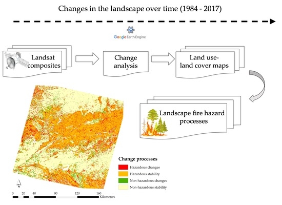
2.3.5. Phase 5: Landscape Fire Hazard Characterization

We detected LULC changes by comparing LULC maps every five years: 1984–1989; 1989–1994; 1994–1999; 1999–2004; 2004–2009; 2009–2014; and 2014–2017. To characterize the hazardousness of the landscape, we reclassified the original LULC types into two classes based on previous studies [7,8,9,73,74]: (i) Hazardous LULC types: pastures, shrublands, open forests, coniferous, and mixed forests; and (ii) nonhazardous LULC types: bare areas, croplands, agroforestry areas, and broadleaved forests. Moreover, to estimate if LULC changes led to a greater or lesser landscape fire hazard, we classified LULC changes for each five-year period into the following change processes: (i) nonhazardous LULC changes: artificialization, agriculture intensification, nonhazardous forest conversion, nonhazardous densification, nonhazardous afforestation, and nonhazardous stability; and (ii) hazardous LULC changes: deforestation, burning degradation, degradation, hazardous forest conversion, encroachment by regeneration and by agriculture abandonment, hazardous densification, hazardous afforestation, and hazardous stability (for a more in-depth explanation see Appendix B,

Table A2. LULC change processes categorized by their hazardousness to fire.

Type	LULC Change	From	To
Nonhazardous changes	Artificialization	All LULC types	Bare areas
	Agriculture intensification	All LULC types	Croplands ( nonirrigated, irrigated or woody crops)
			Agroforestry areas
			Pastures
	Nonhazardous stability	Croplands (nonirrigated, irrigated or woody crops)	Croplands (nonirrigated, irrigated or woody crops)/Agroforestry areas
		Agroforestry areas	Agroforestry areas/ Croplands (nonirrigated, irrigated or woody crops)
		Bare areas	Bare areas
		Broadleaved Forest	Broadleaved Forest
	Nonhazardous forest conversion	Forest (coniferous, mixed and open)	Broadleaved Forest
	Nonhazardous densification	Open Forest	Broadleaved Forest
	Nonhazardous afforestation	Croplands (nonirrigated, irrigated or woody crops)	Broadleaved Forest
		Pastures
		Shrublands
Hazardous changes	Deforestation	Agroforestry areas	Shrublands/pastures/burnt areas
		Broadleaves Forest	Open forests/shrublands/pastures
		Forest (coniferous, mixed and open)	Open forests/shrublands/pastures
	Burning degradation	All LULC types	Burnt areas
	Degradation	Shrublands	Pastures
	Hazardous forest conversion	Mixed Forest	Coniferous forest
	Encroachment	Burnt areas/bare areas	Pastures, Shrublands
	Agriculture abandonment	Croplands (nonirrigated, irrigated or woody crops)	Pastures/shrublands
		Agroforestry areas	Open forests/shrublands/pastures
		Pastures	Shrublands
	Hazardous densification	Open Forest	Forest (coniferous and mixed)
		Shrublands	Open Forest
	Hazardous afforestation	Croplands (nonirrigated, irrigated or woody crops)	Forest (coniferous, mixed and open)
		Agroforestry areas
		Pastures
		Shrublands
	Hazardous stability	Forest (coniferous, mixed and open)	Forest (coniferous, mixed and open)

).

3. Results

3.1. Landsat Images Composites

In 64.7% of the years considered it was possible to create the image composites using pixels acquired within the target year and months (July–August–September). However, in 17.6% of cases, we used pixels acquired one year before or after the target year to cover small areas that remained without data. Specifically, the years 2004 and 2012 had areas without data, due to the failures of the Landsat 7 sensor. In addition, in approximately 17% of the years evaluated, it was not necessary to make a composite image, since there was a single image with 0% cloud cover captured within the target time window. Approximately 55% of the pixels in the time series were acquired in August, 39% in September, and 5% in July. Figure 3 shows an example of the image composite generated for the year 2003.

3.2. Change Analysis

From the temporal segmentation performed using the LT and FT algorithms, we identified: (i) stable areas where the spectral response of the pixel did not change during the entire LTS; therefore, we assigned a single LULC class during the entire period (Figure 4a), (ii) recovery areas with positive slope (Figure 4b), and (iii) disturbed areas with negative slope, which were indicated as breakpoints or abrupt changes in the spectral trajectory of the pixel (Figure 4c,d) [75].

The spatial pattern of disturbance and recovery, using the FT algorithm, was rendered as a gradient according to the change magnitude, showing smooth and abrupt changes from the initial year up to any year of the series. For the year 2003, which was a year with a high number of large fires in our study area, the resulting map showed that in the north, disturbance and recovery events were associated with agricultural activities; in the central zone, the changes were predominantly abrupt and short-term, mostly caused by fires, while stable zones were distributed throughout the study area, occurring mainly in bare areas, grasslands, and shrublands (Figure 5).

The simple relationship between the fires detected by MODIS and the fires detected by LT and FT indicates that the FT algorithm detected 95% of MODIS fires, while the LT algorithm detected 83% of them. In terms of area ratio, FT was able to detect 64.9% of the fire areas, whereas LT only 34.46%, which indicated that LT had a lower ability to identify low-severity burned areas. It is important to note that LT and FT can detect burned areas below the MODIS size detectability threshold, however, if the spectral signal of change is light, neither LT nor FT will be able to detect it. Moreover, when MODIS detects any burn pixel located on the edge of the fire or on a non-burning island within the fire, it can overestimate the burn area with respect to Landsat because of its large pixel size (500 m versus 30 m). Accordingly, the area detected by MODIS was always slightly larger than the burned area detected by the LT and FT algorithms, resulting in commission errors in the MCD64A1 burned area maps (Figure 6).

3.3. Training and Validation Points

The spectral separability analysis performed using the Jeffries Matusita (JM) distance (Appendix C,

Table A3. The spectral separability analysis using the Jeffries Matusita (JM) distance for the 1985 classification.

Class	Nonirrigated Crops	Irrigated Crops	Burnt	Woody Crops	Agroforestry	Pastures	Broadleaved	Coniferous	Mixed	Shrublands	Open Forest	Bare Areas
Nonirrigated crops	0.0
Irrigated crops	1407.6	0.0
Burnt	1411.9	1414.1	0.0
Woody Crops	1241.5	1348.9	1409.9	0.0
Agroforestry	1319.2	1403.3	1410.9	1003.9	0.0
Pastures	1211.4	1403.9	1412.9	1056.4	902.7	0.0
Broadleaved	1411.1	1231.1	1413.8	1341.5	1381.6	1397.2	0.0
Coniferous	1413.1	1393.4	1406.4	1390.3	1395.1	1412.0	1301.7	0.0
Mixed	1412.7	1409.1	1409.5	1374.8	1360.3	1406.5	1355.0	1201.9	0.0
Shrublands	1373.0	1400.6	1380.5	1175.2	1050.1	1288.9	1360.6	1288.5	1208.1	0.0
Open forest	1408.7	1360.6	1410.6	1306.7	1332.0	1392.9	1090.9	1096.6	982.4	1178.9	0.0
Bare Areas	1165.7	1408.2	1386.8	1107.9	1265.0	1281.4	1409.4	1403.9	1403.8	1259.8	1394.6	0.0

* Note: JM values range from 0 to 1414. A JM value of 1414 suggests excellent class separation. A value above 1300 provides good separation, while below 1100 there is low separability.

), and the spectral dispersion diagrams between pairs of bands (Appendix C, Figure A2), indicated that despite the accurate sampling of LULC classes, open woods and mixed forests had similar spectral signatures to conifer and broadleaved forests as well as to woody crops (JM distance values between 900 and 1100). Additionally, the spectral response of pastures showed a low separability with shrublands, agroforestry areas, and nonirrigated croplands.

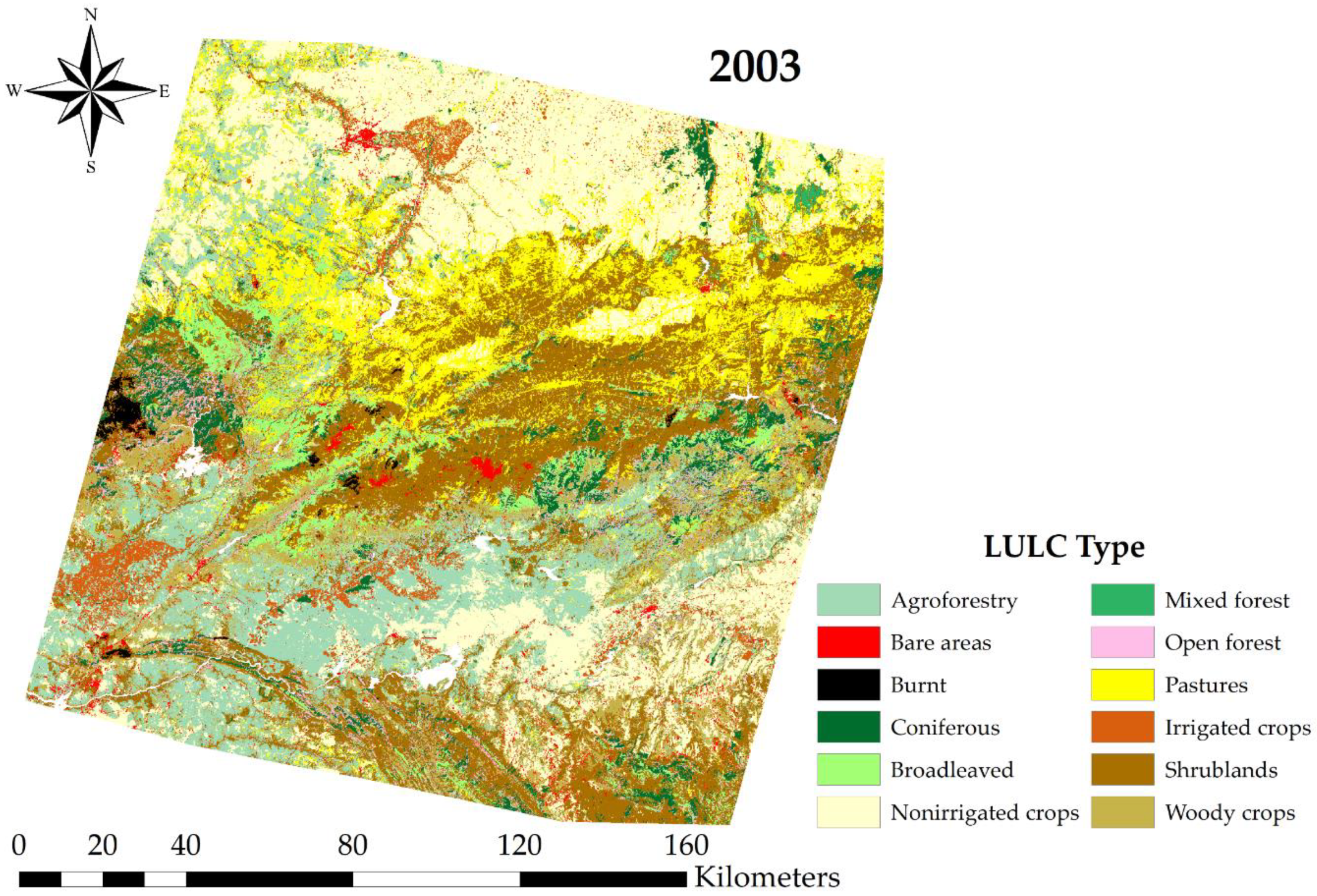
3.4. Annual LULC Maps

The overall accuracy of LULC maps using the three classification methods was rather high for the entire time series (

Table 1. Overall accuracy of the Landsat Time Series (LTS) classification using different methods.

General Accuracy of the Classification (%)
Method 1: Spectral Information + Vegetation Indices + Elevation + Slope	81.11 ± 0.043
Method 2: Variables of Method 1 + Change Metrics generated by FormaTrend	85.07 ± 0.012
Method 3: Variables of Method 1 + Change metrics generated by LandTrendr	84.23 ± 0.014

). Method 1 (spectral information + vegetation indices + elevation + slope) showed the lowest accuracy (81.11%). Method 2 (variables of Method 1 + change metrics generated by FT) increased the accuracy of the classification to 85.07%. However, Method 3 (variables of Method 1 + change metrics generated by LT), slightly decreased the classification accuracy of Method 2 to 84.23% (see Appendix D, Figure A3 to view the LULC map for 2003).

To assess the relative importance of each explanatory variable, we carried out RF classifications with single variables (not shown). From these models, we observed that none of the variables alone explained more than 60% of the spectral variability of the LULC types. According to this, we included, step by step, only the variables which were able to increase the accuracy of the classification. Regarding the additive accuracy, we found that Red and NIR were the variables which gave greater accuracy to the classification (34% and 23% respectively), followed by SWIR-1 (10%), and slope (5%) (

Table 2. Overall accuracy of the classification for different methods.

Number of Bands/Indices/Change Metrics	Band/ Index/Change Metrics Set	Overall Accuracy
1	Red	0.34
2	Red, NIR	0.57
3	Red, NIR, SWIR	0.67
4	Red, NIR, SWIR-1, SWIR-2	0.69
7	Red, NIR, SWIR-1, SWIR-2, TCB, TCG, TCW	0.71
8	Red, NIR, SWIR-1, SWIR-2, TCB, TCG, TCW, NBR	0.73
9	Red, NIR, SWIR-1, SWIR-2, TCB, TCG, TCW, NBR, NDVI	0.72
10	Red, NIR, SWIR-1, SWIR-2, TCB, TCG, TCW, NBR, NDVI, Slope	0.77
11	Red, NIR, SWIR-1, SWIR-2, TCB, TCG, TCW, NBR, NDVI, slope, elevation	0.81
14	FT variables: Red, NIR, SWIR-1, SWIR-2, TCB, TCG, TCW, NBR, NDVI, slope, elevation, type, mag, dir.	0.85
17	LT variables: Red, NIR, SWIR-1, SWIR-2, TCB, TCG, TCW, NBR, NDVI, slope, elevation, type, mag, dir, dur, year, prechange	0.84

). Furthermore, the variables elevation, change magnitude (mag), change direction (dir) and change type (type) were included in the group of good predictors because they increased the accuracy of the LULC maps by 4%. Variables with a lower impact on the classification, but that also increased accuracy were: NBR, brightness, greenness, and wetness. By contrast, the NDVI, change year (year) and prechange spectral value showed a slightly negative effect on the accuracy of the classification (Table 2).

In general, omission errors were lower than commission errors in all the years. Open wood, mixed forests, and pastures were the LULC types that showed the most omission and commission errors in the classifications using Methods 2 and 3. However, Method 2 (Figure 7a) had less omission and commission errors in all LULC classes compared to Method 3 (Figure 7b). Based on these results, we selected Method 2 (i.e., variables of method 1 + change metrics generated by FT) to produce the annual LULC maps, to characterize the dynamics of change over the last 34 years, and to assess changes in landscape fire hazard.

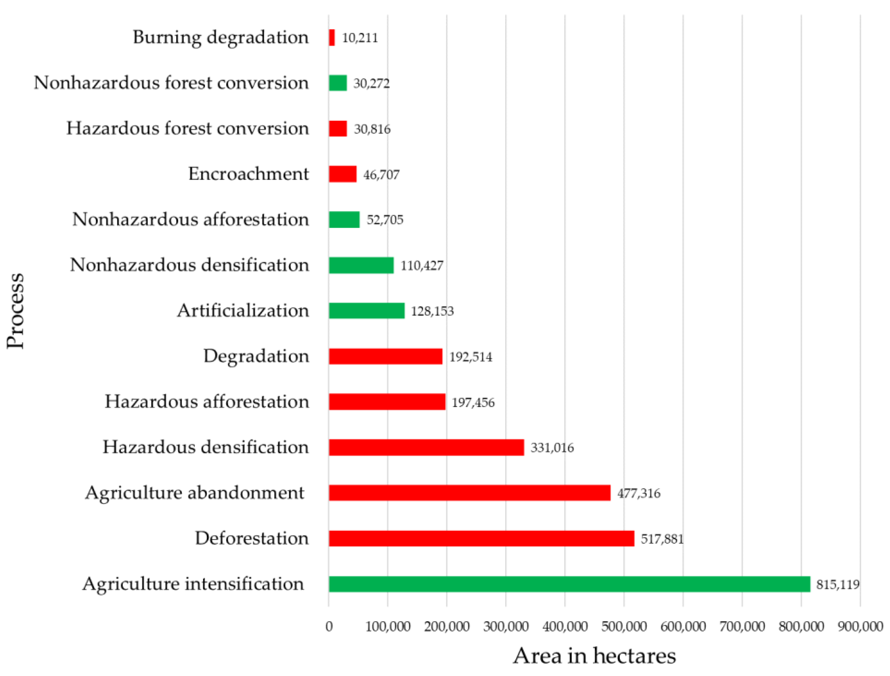
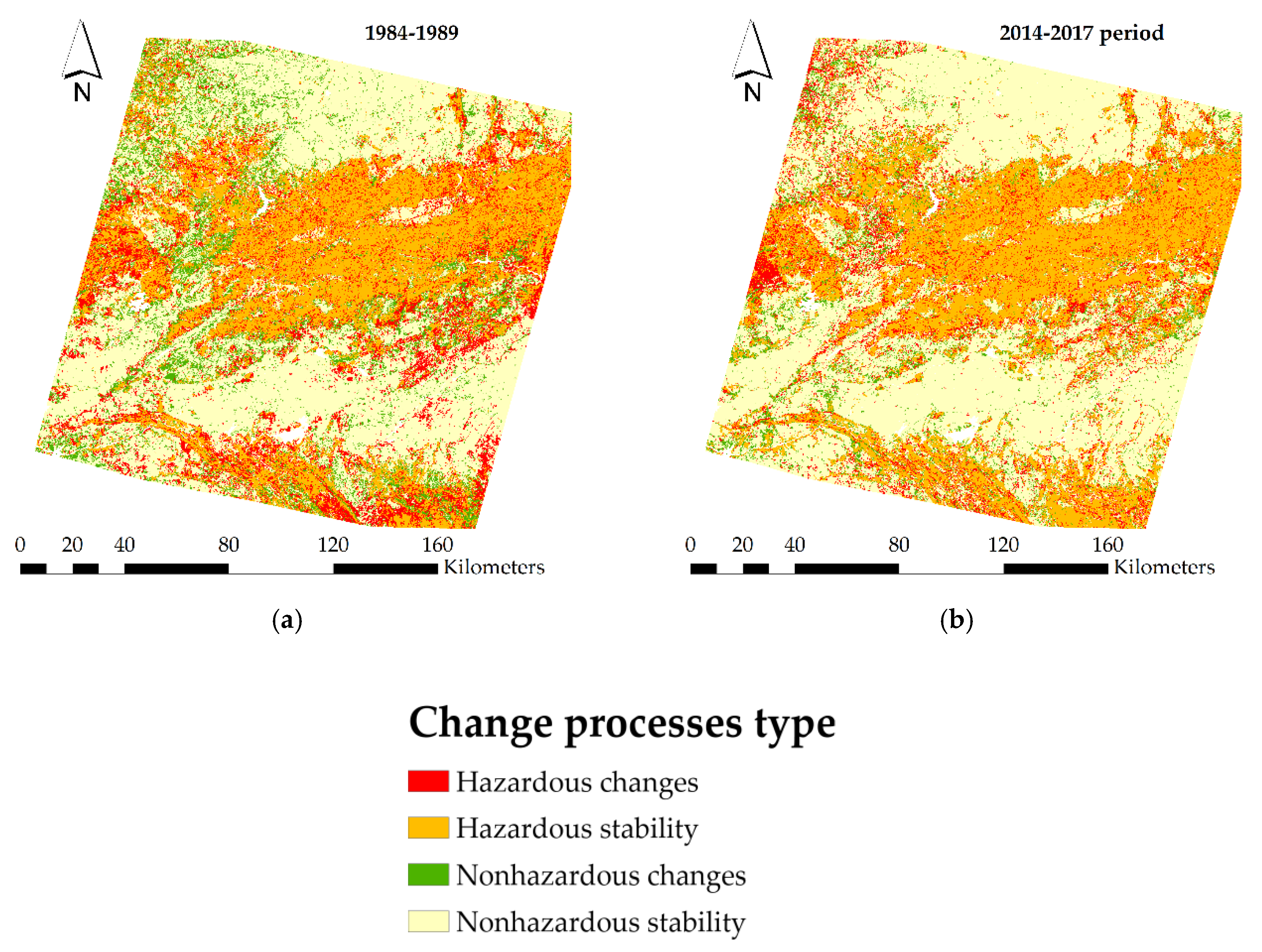
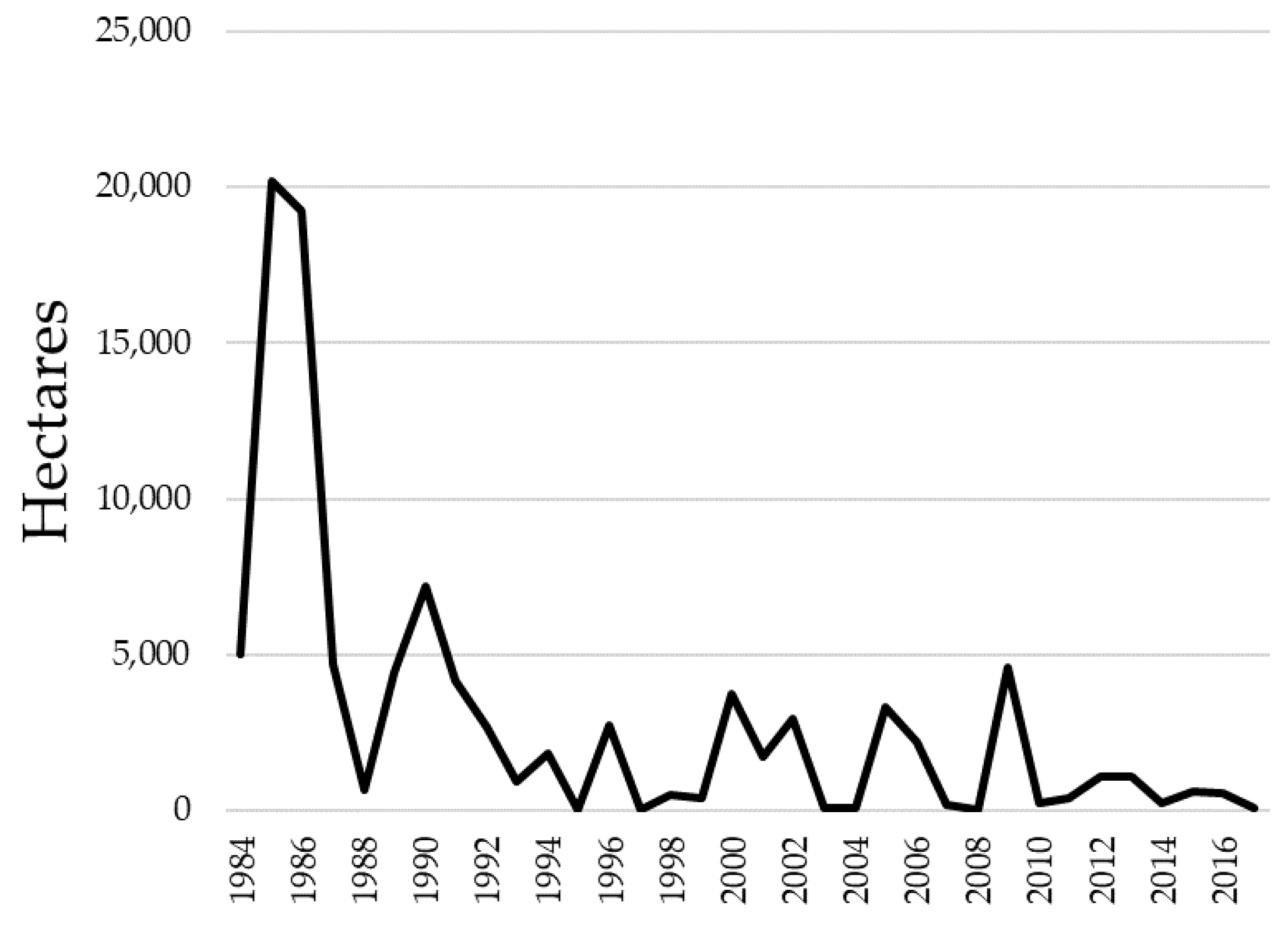
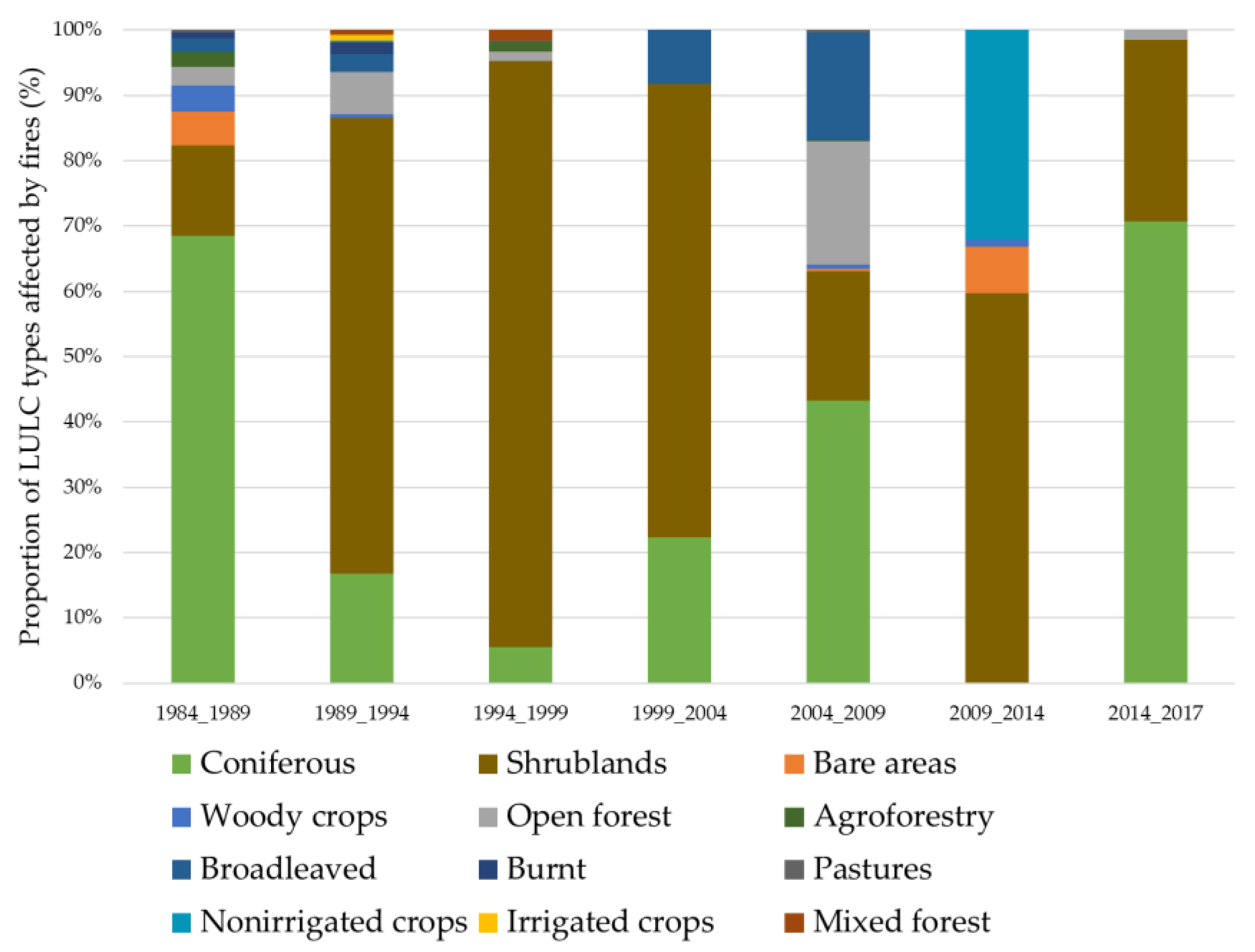
3.5. Landscape Fire Hazard Characterization

In absolute terms, the landscape was rather stable, since the areas that did not change occupied approximately 80% of the total surface, increasing over time (varying from 74% in the period 1984–1989 to 82% in 2014–2017). In this context, nonhazardous stable LULC classes occupied 45–49% of the total area, and hazardous ones covered 28–33% during the study period. Nevertheless, more than 20% of the territory experiencing changes was a considerable value.

Regarding LULC changes experienced during the 34 years of study, more area was affected by processes that increased landscape fire hazard (1,803,917 ha) than by those that decreased it (1,136,676 ha). The most important nonhazardous LULC change was agrarian intensification, while artificialization and nonhazardous densification were less abundant (Figure 8). On the other hand, the most important hazardous LULC changes during the entire period were deforestation, agriculture abandonment, hazardous densification, hazardous afforestation, and degradation. The processes that increased the hazardousness of the landscape were spatially aggregated at the eastern and western edges of our study area, where conifers and shrublands predominate. To the contrary, the processes that decreased landscape hazard were concentrated mainly in the center and north of the study area (Figure 9, see Appendix E, Figure A4 for the entire series of maps).

The rate of change of the hazardous and nonhazardous LULC processes decreased over time. Among nonhazardous changes, agrarian intensification was the only process that showed a significant trend, with a rate of change which varied from 8% in the first five-year period (1984–1989) to 5.4% in the last five-year period (2014–2017). Similarly, several LULC hazardous rates of change were reduced: deforestation rates went from 4.6% to 3.3%, and encroachment by agricultural abandonment from 4% to 2.6%. The remaining hazardous processes (i.e., hazardous densification, hazardous afforestation, and degradation) had very low rates of change (< 2.5%) over time (Figure 10).

The area affected by fires decreased over time. The most affected years by fires were 1985 (with approximately 20,166 ha burned), followed by 1986 (19,215 ha) and 1990 (7,218 ha) (Figure 11). During the periods 1989–1994, 1994–1999, 1999–2004, and 2009–2014, the LULC type most affected by fire was shrublands (70%, 90%, 69%, and 59% in each period, respectively), while during the periods 1984–1989, 2004–2009, and 2014–2017, the LULC type with the greatest area burned was coniferous forest (69%, 43%, and 70% respectively). In general, these two LULC types were the most affected by fires in all the years under study (Figure 12).

4. Discussion

4.1. Methodological Issues

In order to maximize classification accuracy, input images must have minimal contamination from clouds, haze, or shadows, as these are an important obstacle to studying the ground surface [76]. In this study, we used a simple and robust statistics-based composites method (“medoid”) that does not need to set parameters and could be automated for application into very large data collections and time series. In spite of the potential offered by the “medoid” technique, the resulting image collection presented areas without information. This situation underlines the need to complement the analysis with other sensors with similar spectral and spatial characteristics (e.g., Sentinel 2 available from 2015) [29].

Regarding the change analysis, we demonstrate the utility of LT and FT algorithms to detect LULC changes in our study area. However, as with automated algorithms, there are some limitations in their application. For example, FT, in contrast to LT, does not have the ability to generate metrics that are very useful when studying the postdisturbance regeneration, such as year, duration of change, and the spectral values before the change. The LT algorithm, although generating these metrics in some years of the time series, can present misidentified change events (omission errors) [77,78,79] and false detections (commission errors) [39]. Therefore, studies interested in obtaining the most accurate time segmentation have performed the LTS analysis using methodologies that allow greater control by the user, either through human interpretation [27], or by using algorithms such as TimeSync [80]. Our results indicate that LT had a lower ability to detect low severity burned areas, compared to the FT algorithm. These results may be mainly caused by the effect of residual interannual noise (e.g., phenology, sun-angle, and residual atmospheric effects), and because LT is a complex system with many control parameters, and therefore is very sensitive to inaccurate calibration. Thus, it is recommended to perform a true sensitivity analysis or parameter optimization more exhaustive than the one performed in this study, to determine how changing those parameters and the spectral transformations used in the detection of changes affects final outcomes. These results have to be taken with caution because we compared the LT and FT results with the MCD64A1 burned area product derived from the MODIS satellite, which has lower resolution than Landsat. Thus, the minimum size of a land cover change detectable with Landsat data is much smaller than that detectable with MODIS. In this respect, a more precise approach would be a validation method using independent data taken from sensors with the same or higher resolution than that available from Landsat.

Moreover, to improve the spectral separability of complex LULC types and to perform a consistent spectral characterization over time, we collected space-time reference samples reducing the spectral-temporal variability [81]. For this purpose, a stratified random sampling only on the stable areas throughout the time series, allowed us to keep fixed most of the training and validation points during all the years, increasing the efficiency of the sampling process. In addition, we included “auxiliary data” related to the topography (elevation and slope) improving our classification, mainly because the spatial patterns of vegetation in Sierra de Gredos is highly influenced by topography [56]. Apart from topography, it is possible to include additional auxiliary data to increase the accuracy of LULC mapping or even to classify them as fuel complexes, such as LiDAR (Light Detection and Ranging), hyperspectral, and environmental data, such as bioclimatic regions (precipitation and temperature) [82]. This type of information has led to a significant increase in the overall LULC classification accuracy relative to the pure spectral information input [83,84]. However, the LiDAR data are often limited to the last years of the time series; therefore, only auxiliary data that are both available and consistent over time should be included. Moreover, processing LiDAR data over large areas is rather impractical due to the high data volume.

In the LULC classification and validation phase, we demonstrate that information about the type of change (disturbance or recovery) and its magnitude and direction, derived from the FT and LT algorithms, are important variables for predicting the LULC types and that those variables increased the overall accuracy of our LULC maps by 4%, compared to the classification of single date spectral variables. This confirms previous works [25,33,40,75] that indicated that the LULC composition at any point in time is linked to past disturbance and recovery events, so that change is not simply a contrast between conditions at two times points, but a continuous process that operates at both rapid (abrupt changes) and slow (gradual changes) rates in the landscape. However, some metrics from the LT algorithm, such as the time in which the change occurs (year), the duration of the change (dur) and the spectral value prior to the change (prechange) had a slightly negative effect on the accuracy of the classification. This was contrary to the results obtained by Franklin et al. 2015 [33] who used change metrics to increase the accuracy of the LULC maps in a managed forest area in south-eastern Canada, finding that the change metrics magnitude and duration were important variables for their LULC classification. Therefore, it is evidenced that the importance of the variables can change with the type of landscape, being convenient to separately analyze the applicability of each one of the variables in other study areas. Future research will evaluate the utility of the other change metrics (e.g., duration, year, and prechange) to study the postdisturbance regeneration rate, depending on the different LULC types.

4.2. Changes in Landscape Fire Hazard

In absolute terms, approximately 20% of the landscape has changed during the study period. In terms of nonhazardous changes, we found that the agrarian intensification homogenized the northern and south-eastern areas of our landscape, with large areas dedicated to intensive agriculture. Regarding hazardous changes, deforestation, agriculture abandonment, and hazardous densification by conifers were the most salient changes, which appear to considerably affect fire activity. In our study area, the most affected LULC types by fires were conifer forests and shrublands, which confirms the results indicated by Moreno et al. 2011 [6] in the same study area, in which fire showed positive selectivity for these LULC types. These results also validate the characterization of hazardous change processes in Mediterranean landscapes by several previous authors [7,8,9,73,74,85]. Here, the increase of conifer forests occurred due to both hazardous afforestation and hazardous densification. This increase began in the second half of the twentieth century, due to the forest management of that time [86]. These monospecific pine stands from anthropogenic origin have been more sensitive to fires and have favored large and intense fires [87], whereas broadleaved forests have been able to cope well with current and past fire regimes, although a recent trend toward higher fire occurrences has been observed [54]. Shifts from pine-dominated to oak-dominated stands may play an important role in further reducing overall landscape fire hazard by offering enhanced firefighting opportunities [7]. For example, in areas where coniferous forests are known to burn the most, intermingling with mixed or broadleaved forests could be an effective way to reduce fire spread [5]. Moreover, the densification of open forests and agroforestry areas, due to the abandonment of traditional forest practices such as grazing, have augmented the extension of dense conifer or mixed forests. In addition, the proliferation of shrublands as a result of encroachment, due to both regeneration of burned areas and agriculture abandonment, have increased the spatial continuity of hazardous vegetation, which might have favored fire spread [5,9,88].

In this sense, although a decrease in fire activity has been observed, this trend does not necessarily imply that the landscape is less hazardous. On the contrary, the continued abandonment of traditional agriculture activities implies that there is a currently greater wildfire risk due to the build-up of large and continuously growing vegetation prone to burn [5,9]. A common practice before agricultural abandonment in the 1970s was to maintain and improve pastures to avoid encroachment through proper management of livestock [89]. Livestock played an important role in firefighting that was interrupted when crop cultivation/plant production was separated from livestock in the second half of the twentieth century, and most notably in the 1970s, linked to the incentive system of the European Union agricultural policy [9,86]. This resulted in the proliferation of large fires in the area, as happened in 1985. Afterwards, the use of fire was regulated and prohibited in times of high risk, and new efficient firefighting services were implemented [15,54], such that fires have progressively decreased. However, in a context of increased extreme fire weather conditions due to global warming, the fire regime could shift to more severe fires. Current firefighting capacity may be overridden when wind, topography, high fuel load, and fuel continuity facilitate fire propagation [90].

Moreover, although LULC stability was dominant, this did not mean that fire hazardousness had not increased in the landscape over time [9,91]. Stability through time in terms of land cover does not necessarily mean stability of other vegetation properties related to flammability, as they may change with age, or the accumulation of litter in conifer forests [88,92], which increases susceptibility to fire over time [93]. For burned areas, shrublands that develop after a fire can reach almost continuous coverage in a few years, as well as accumulate large amounts of highly flammable biomass [94]. Consequently, the evaluation of the interaction between fires and landscape should not be limited only to the analysis of the spatial occupation of LULC types, since the structure and state of the vegetation must also be taken into account. Future research will consist of prioritizing representative areas, with different bioclimatic and vegetation characteristics, to characterize and compare fuel types, using LULC types and LiDAR data, which could facilitate valuable information regarding vegetation height and structure.

5. Conclusions

Spectral trajectories and change metrics derived from LandTrendr (LT) and FormaTrend (FT) algorithms have allowed a robust and consistent spectral characterization of LULC types over time. In addition, this type of analysis also increased the accuracy of the LULC classification. However, some of the change metrics have had a slightly negative effect on the classification, suggesting that the real potential of these metrics is the analysis of postdisturbance dynamics rather than being just another variable in the classification process. In addition to this, we found that the FT algorithm had a greater ability than the LT algorithm to identify low-severity fire disturbances. Nevertheless, the LT algorithm, unlike the FT algorithm, generates change metrics that are very useful when studying the dynamics of postdisturbance regeneration of vegetation, such as year, duration of change, and the spectral values before the change. Moreover, the Google Earth Engine (GEE) has proved to be a powerful free access tool to automate processes for image composition, change metrics generation, and LULC maps classification, as well as having advanced algorithms and an extensive data catalogue which is accessible and easy to use. This is important because it reduces the need to download and store large amounts of data.

In relation to the landscape dynamics, we found that the most important change processes during the study period were agrarian intensification, deforestation, encroachment by abandonment, and hazardous densification. However, these changes have slowed down, increasing the extension of stable areas over time. We also observed that the incidence of fires has decreased over time, after peaking in 1985, in spite of an increase of risk factors, including climate change. That means that the recent trend in fire activity is being largely decoupled from trends in climate and landscape hazard, suggesting that fire suppression efforts have been effective. The most affected LULC types by fire were mainly conifer forests and shrublands. In this context, fire management should focus on those vegetation types, favoring silvopastoral practices and afforestation with fire-resistant and resilient species. Although LULC maps are an excellent tool to support long-term fire prevention planning, it is important that this information is complemented with spatially continuous information relative to the vertical structure of vegetation (e.g., height, biomass, diameter, and crown volume), as these characteristics are important for fire propagation and behavior. With the vegetation structure data, it will be possible to obtain a deeper knowledge of the interaction between the landscape and forest fires, complementing the spectral information of satellite images about the severity of change and regenerative dynamics. All of this may contribute to the improvement of fire management plans in the study area.

References

1. Keeley, J.; Bond, W.; Bradstock, R.; Pausas, J.; Rundel, P. Fire in Mediterranean Ecosystems: Ecology, Evolution and Management; Cambridge University Press: Cambridge, UK, 2011; pp. 1–515. [Google Scholar]
2. Pausas, J.G.; Llovet, J.; Rodrigo, A.; Vallejo, R. Are wildfires a disaster in the Mediterranean basin?—A review. Int. J. Wildl. Fire 2008, 17, 713–723. [Google Scholar] [CrossRef]
3. Martínez, J.; Vega-Garcia, C.; Chuvieco, E. Human-caused wildfire risk rating for prevention planning in Spain. J. Environ. Manag. 2009, 90, 1241–1252. [Google Scholar] [CrossRef]
4. Le Houerou, H.N. Fire and vegetation in the Mediterranean basin. In Plant Production and Protection Division; FAO-Rome: Rome, Italy, 1974; pp. 237–277. ISBN 0082-1527. [Google Scholar]
5. Oliveira, S.; Moreira, F.; Boca, R.; San-Miguel-Ayanz, J.; Pereira, J.M.C. Assessment of fire selectivity in relation to land cover and topography: A comparison between Southern European countries. Int. J. Wildl. Fire 2014, 23, 620–630. [Google Scholar] [CrossRef]
6. Moreno, J.M.; Viedma, O.; Zavala, G.; Luna, B. Landscape variables influencing forest fires in central Spain. Int. J. Wildl. Fire 2011, 20, 678–689. [Google Scholar] [CrossRef] [Green Version]
7. Moreira, F.; Vaz, P.; Catry, F.; Silva, J.S. Regional variations in wildfire susceptibility of land-cover types in Portugal: Implications for landscape management to minimize fire hazard. Int. J. Wildl. Fire 2009, 18, 563–574. [Google Scholar] [CrossRef]
8. Fernandes, P.M. Fire-smart management of forest landscapes in the Mediterranean basin under global change. Landsc. Urban Plan. 2013, 110, 175–182. [Google Scholar] [CrossRef] [Green Version]
9. Viedma, O.; Moity, N.; Moreno, J.M. Changes in landscape fire-hazard during the second half of the 20th century: Agriculture abandonment and the changing role of driving factors. Agric. Ecosyst. Environ. 2015, 207, 126–140. [Google Scholar] [CrossRef]
10. Pausas, J.G.; Fernández-Muñoz, S. Fire regime changes in the Western Mediterranean Basin: from fuel-limited to drought-driven fire regime. Clim. Chang. 2012, 110, 215–226. [Google Scholar] [CrossRef]
11. Moreira, F.; Rego, F.C.; Ferreira, P.G. Temporal (1958–1995) pattern of change in a cultural landscape of northwestern Portugal: Implications for fire occurrence. Landsc. Ecol. 2001, 16, 557–567. [Google Scholar] [CrossRef]
12. Bedia, J.; Herrera, S.; Camia, A.; Moreno, J.; Gutiérrez, J. Forest Fire Danger Projections in the Mediterranean using ENSEMBLES Regional Climate Change Scenarios. Clim. Chang. 2014, 122, 185–199. [Google Scholar] [CrossRef]
13. Turco, M.; Bedia, J.; Di Liberto, F.; Fiorucci, P.; Von Hardenberg, J.; Koutsias, N.; Llasat, M.C.; Xystrakis, F.; Provenzale, A. Decreasing fires in Mediterranean Europe. PLoS ONE 2016, 11, e0150663. [Google Scholar] [CrossRef]
14. Brotons, L.; Aquilué, N.; de Cáceres, M.; Fortin, M.J.; Fall, A. How Fire History, Fire Suppression Practices and Climate Change Affect Wildfire Regimes in Mediterranean Landscapes. PLoS ONE 2013, 8, e62392. [Google Scholar] [CrossRef]
15. Ruffault, J.; Mouillot, F.; Peters, D.P.C. How a new fire-suppression policy can abruptly reshape the fire-weather relationship. Ecosphere 2015, 6, 1–19. [Google Scholar] [CrossRef]
16. Urbieta, I.R.; Zavala, G.; Bedia, J.; Gutiérrez, J.M.; Miguel-Ayanz, J.S.; Camia, A.; Keeley, J.E.; Moreno, J.M.; San Miguel-Ayanz, J.; Camia, A.; et al. Fire activity as a function of fire–weather seasonal severity and antecedent climate across spatial scales in southern Europe and Pacific western USA. Environ. Res. Lett. 2015, 10, 114013. [Google Scholar] [CrossRef]
17. Cardil, A.; Eastaugh, C.S.; Molina, D.M. Extreme temperature conditions and wildland fires in Spain. Theor. Appl. Climatol. 2015, 122, 219–228. [Google Scholar] [CrossRef]
18. Turco, M.; Llasat, M.C.; von Hardenberg, J.; Provenzale, A. Climate change impacts on wildfires in a Mediterranean environment. Clim. Chang. 2014, 125, 369–380. [Google Scholar] [CrossRef]
19. Viedma, O.; Angeler, D.G.; Moreno, J.M. Landscape structural features control fire size in a Mediterranean forested area of central Spain. Int. J. Wildl. Fire 2009, 18, 575–583. [Google Scholar] [CrossRef]
20. Pausas, J.G.; Paula, S. Fuel shapes the fire-climate relationship: Evidence from Mediterranean ecosystems. Glob. Ecol. Biogeogr. 2012, 21, 1074–1082. [Google Scholar]
21. Wulder, M.A.; White, J.C.; Goward, S.N.; Masek, J.G.; Irons, J.R.; Herold, M.; Cohen, W.B.; Loveland, T.R.; Woodcock, C.E. Landsat continuity: Issues and opportunities for land cover monitoring. Remote Sens. Environ. 2008, 112, 955–969. [Google Scholar] [CrossRef]
22. Roder, A.; Hill, J.; Hostert, P. Radiometric intercalibration of Landsat-TM and—MSS data for quantitative long-term environmental monitoring. In Proceedings of the EARSeL 20th Symposium—A Decade of Trans-European Remote Sensing Cooperation, Dresden, Germany, 14–16 June 2001; pp. 1–28. [Google Scholar]
23. Hansen, M.C.; Roy, D.P.; Lindquist, E.; Adusei, B.; Justice, C.O.; Altstatt, A. A method for integrating MODIS and Landsat data for systematic monitoring of forest cover and change in the Congo Basin. Remote Sens. Environ. 2008, 112, 2495–2513. [Google Scholar] [CrossRef]
24. Giglio, L.; Boschetti, L.; Roy, D.P.; Humber, M.L.; Justice, C.O. The Collection 6 MODIS burned area mapping algorithm and product. Remote Sens. Environ. 2018, 217, 72–85. [Google Scholar] [CrossRef]
25. Hermosilla, T.; Wulder, M.A.; White, J.C.; Coops, N.C.; Hobart, G.W.; Campbell, L.B. Mass data processing of time series Landsat imagery: Pixels to data products for forest monitoring. Int. J. Digit. Earth 2016, 9, 1035–1054. [Google Scholar] [CrossRef]
26. Matasci, G.; Hermosilla, T.; Wulder, M.A.; White, J.C.; Coops, N.C.; Hobart, G.W.; Bolton, D.K.; Tompalski, P.; Bater, C.W. Three decades of forest structural dynamics over Canada’s forested ecosystems using Landsat time-series and lidar plots. Remote Sens. Environ. 2018, 216, 697–714. [Google Scholar] [CrossRef]
27. Potapov, P.V.; Turubanova, S.A.; Hansen, M.C.; Adusei, B.; Broich, M.; Altstatt, A.; Mane, L.; Justice, C.O. Quantifying forest cover loss in Democratic Republic of the Congo, 2000–2010, with Landsat ETM + data. Remote Sens. Environ. 2012, 122, 106–116. [Google Scholar] [CrossRef]
28. Flood, N. Seasonal composite Landsat TM/ETM + Images using the medoid (a multi-dimensional median). Remote Sens. 2013, 5, 6481–6500. [Google Scholar] [CrossRef]
29. White, J.C.; Wulder, M.A.; Hobart, G.W.; Luther, J.E.; Hermosilla, T.; Griffiths, P.; Coops, N.C.; Hall, R.J.; Hostert, P.; Dyk, A.; et al. Pixel-based image compositing for large-area dense time series applications and science. Can. J. Remote Sens. 2014, 40, 192–212. [Google Scholar] [CrossRef]
30. Griffiths, P.; van der Linden, S.; Kuemmerle, T.; Hostert, P. A Pixel-Based Landsat Compositing Algorithm for Large Area Land Cover Mapping. IEEE J. Sel. Top. Appl. Earth Obs. Remote Sens. 2013, 6, 2088–2101. [Google Scholar] [CrossRef]
31. Banskota, A.; Kayastha, N.; Falkowski, M.J.; Wulder, M.A.; Froese, R.E.; White, J.C. Forest Monitoring Using Landsat Time Series Data: A Review. Can. J. Remote Sens. 2014, 40, 362–384. [Google Scholar] [CrossRef]
32. Shumway, R.H.; Stoffer, D.S. Time Series Analysis and Applications Using the R Statistical Package, 3rd ed.; Springer: New York, USA, 2011. [Google Scholar]
33. Franklin, S.E.; Ahmed, O.S.; Wulder, M.A.; White, J.C.; Hermosilla, T.; Coops, N.C. Large Area Mapping of Annual Land Cover Dynamics Using Multitemporal Change Detection and Classification of Landsat Time Series Data. Can. J. Remote Sens. 2015, 41, 293–314. [Google Scholar] [CrossRef]
34. Hawbaker, T.J.; Vanderhoof, M.K.; Beal, Y.; Takacs, J.D.; Schmidt, G.L.; Falgout, J.T.; Williams, B.; Fairaux, N.M.; Caldwell, M.K.; Picotte, J.J.; et al. Mapping burned areas using dense time-series of Landsat data. Remote Sens. Environ. 2017, 198, 504–522. [Google Scholar] [CrossRef]
35. Frazier, R.J.; Coops, N.C.; Wulder, M.A.; Hermosilla, T.; White, J.C. Analyzing spatial and temporal variability in short-term rates of post fire vegetation return from Landsat time series. Remote Sens. Environ. 2018, 205, 32–45. [Google Scholar] [CrossRef]
36. Li, X.; Zhou, Y.; Zhu, Z.; Liang, L.; Yu, B.; Cao, W. Mapping annual urban dynamics (1985–2015 ) using time series of Landsat data. Remote Sens. Environ. 2018, 216, 674–683. [Google Scholar] [CrossRef]
37. Hansen, M.C.; Potapov, P.V.; Moore, R.; Hancher, M.; Turubanova, S.A.; Tyukavina, A.; Thau, D.; Stehman, S.V.; Goetz, S.J.; Loveland, T.R.; et al. High-resolution global maps of 21st-century forest cover change. Science 2013, 342, 850–853. [Google Scholar] [CrossRef]
38. Verbesselt, J.; Hyndman, R.; Newnham, G.; Culvenor, D. Detecting trend and seasonal changes in satellite image time series. Remote Sens. Environ. 2010, 114, 106–115. [Google Scholar] [CrossRef]
39. Griffiths, P.; Kuemmerle, T.; Kennedy, R.E.; Abrudan, I.V.; Knorn, J.; Hostert, P. Using annual time-series of Landsat images to assess the effects of forest restitution in post-socialist Romania. Remote Sens. Environ. 2012, 118, 199–214. [Google Scholar] [CrossRef]
40. Kennedy, R.E.; Yang, Z.; Cohen, W.B. Detecting trends in forest disturbance and recovery using yearly Landsat time series: 1. LandTrendr—Temporal segmentation algorithms. Remote Sens. Environ. 2010, 114, 2897–2910. [Google Scholar] [CrossRef]
41. Jamali, S.; Seaquist, J.; Eldundh, L.; Ardo, J.; Eklundh, L.; Ardö, J.; Eldundh, L.; Ardo, J. Automated mapping of vegetation trends with polynomials using NDVI imagery over the Sahel. Remote Sens. Environ. 2014, 141, 79–89. [Google Scholar] [CrossRef]
42. Hammer, D.; Kraft, R.; Zedilllo, E.; Wheeler, D. FORMA: Forest Monitoring for Action—Rapid Identification of Pan-Tropical Deforestation Using Moderate Resolution Remotely Sensed Data; Center for Global Development: Washington, DC, USA, 2009. [Google Scholar]
43. Gorelick, N.; Hancher, M.; Dixon, M.; Ilyushchenko, S.; Thau, D.; Moore, R. Google Earth Engine: Planetary-scale geospatial analysis for everyone. Remote Sens. Environ. 2017, 202, 18–27. [Google Scholar] [CrossRef]
44. FAO-Unesco. Soil Map of the World, Volume V—Europe. In Soil Map of the World; Unesco: Paris, France, 1974; Volume 1, p. 20. [Google Scholar]
45. U.S. Geological Survey. Landsat 4–7 Surface Reflectance (Ledaps) Version 1.0 Product Guide; U.S. Geological Survey: Sioux Falls, SD, USA, 2018.
46. Vermote, E.; Tantre, D.; Deuzé, J.; Herman, M.; Morcrette, J. Second Simulation of the Satellite Signal in the Solar Spectrum, 6S: An Overview. IEEE Trans. Geosci. Remote Sens. 1997, 21, 177–179. [Google Scholar] [CrossRef]
47. U.S. Geological Survey. Landsat 8 Surface Reflectance Code (LaSRC) Version 4.3 Product Guide; U.S. Geological Survey: Sioux Falls, SD, USA, 2018.
48. Andrefouet, S.; Bindschadler, R.; Brown de Colstoun, E.; Choate, M.; Chomentowski, W.; Christopherson, J.; Doorn, B.; Hall, D.; Holifield, C.; Howard, S.; et al. Preliminary Assessment of the Value of Landsat 7 ETM+ Data Following Scan Line Corrector Malfunction; U.S. Geological Survey: Sioux Falls, SD, USA, 2003.
49. Aubard, V.; Paulo, J.A.; Silva, J.M.N. Long-Term Monitoring of Cork and Holm Oak Stands Productivity in Portugal with Landsat Imagery. Remote Sens. 2019, 11, 525. [Google Scholar] [CrossRef]
50. Miller, J.D.; Thode, A.E. Quantifying burn severity in a heterogeneous landscape with a relative version of the delta Normalized Burn Ratio (dNBR). Remote Sens. Environ. 2007, 109, 66–80. [Google Scholar] [CrossRef]
51. Ministerio de Agricultura Pesca y Alimentación (MAPA). Mapa de Cultivos y Aprovechamientos de España. Available online: https://www.mapa.gob.es/es/agricultura/temas/sistema-de-informacion-geografica-de-datos-agrarios/mca.aspx (accessed on 1 February 2019).
52. Ministerio de Transición Ecológica (MITECO). Mapa Forestal de España. Available online: https://www.mapa.gob.es/es/desarrollo-rural/temas/politica-forestal/inventario-cartografia/mapa-forestal-espana/default.aspx (accessed on 1 February 2019).
53. Kosztra, B.; Büttner, G.; Hazeu, G.; Arnold, S. Updated CLC Illustrated Nomenclature Guidelines; European Environment Agency: Wien, Austria, 2017. [Google Scholar]
54. Viedma, O.; Urbieta, I.R.; Moreno, J.M. Wildfires and the role of their drivers are changing over time in a large rural area of west-central Spain. Sci. Rep. 2018, 8, 17797. [Google Scholar] [CrossRef]
55. Ministerio de Fomento. Plan Nacional de Ortofotografía Aérea (PNOA). Available online: http://pnoa.ign.es/ (accessed on 1 February 2019).
56. Viedma, O. The influence of topography and fire in controlling landscape composition and structure in Sierra de Gredos (Central Spain). Landsc. Ecol. 2008, 23, 657–672. [Google Scholar] [CrossRef]
57. Farr, T.G.; Rosen, P.; Caro, E.; Crippen, R.; Duren, R.; Hensley, S.; Kobrick, M.; Paller, M.; Rodriguez, E.; Roth, L.; et al. The shuttle radar topography mission. Rev. Geophys. 2007, 45, 1–33. [Google Scholar] [CrossRef]
58. Viedma, O.; Del campo, P. Cartografía y validación de la superficie quemada de incendios mediante imágenes Landsat TM y ETM ETM + en el centro-oeste de España durante el período 1985–2009. Rev. Montes 2016, 124, 5–12. [Google Scholar]
59. Roberts, D.; Mueller, N.; McIntyre, A. High-Dimensional Pixel Composites from Earth Observation Time Series. IEEE Trans. Geosci. Remote Sens. 2017, 55, 6254–6264. [Google Scholar] [CrossRef]
60. Kennedy, R.E.; Yang, Z.; Gorelick, N.; Braaten, J.; Cavalcante, L.; Cohen, W.B.; Healey, S. Implementation of the LandTrendr algorithm on Google Earth Engine. Remote Sens. 2018, 10, 691. [Google Scholar] [CrossRef]
61. Myneni, R.B.; Hall, F.G.; Sellers, P.J.; Marshak, A.L. Interpretation of spectral vegetation indexes. IEEE Trans. Geosci. Remote Sens. 1995, 33, 481–486. [Google Scholar] [CrossRef]
62. Pettorelli, N.; Vik, J.O.; Mysterud, A.; Gaillard, J.M.; Tucker, C.J.; Stenseth, N.C. Using the satellite-derived NDVI to assess ecological responses to environmental change. Trends Ecol. Evol. 2005, 20, 503–510. [Google Scholar] [CrossRef]
63. Lentile, L.B.; Holden, Z.A.; Smith, A.M.S.; Falkowski, M.J.; Hudak, A.T.; Morgan, P.; Lewis, S.A.; Gessler, P.E.; Benson, N.C. Remote sensing techniques to assess active fire characteristics and post-fire effects. Int. J. Ofwildl. Fire 2006, 15, 319–345. [Google Scholar] [CrossRef]
64. Huang, C.; Wylie, B.; Yang, L.; Homer, C.; Zylstra, G.; Yang, W.L.; Homer, C. Derivation of a tasselled cap transformation based on Landsat 7 at-satellite reflectance. Int. J. Remote Sens. 2002, 23, 1741–1748. [Google Scholar] [CrossRef]
65. Cohen, W.B.; Yang, Z.; Healey, S.P.; Kennedy, R.E.; Gorelick, N. A LandTrendr multispectral ensemble for forest disturbance detection. Remote Sens. Environ. 2018, 205, 131–140. [Google Scholar] [CrossRef]
66. Braayen, J.; Kennedy, R.E. LT-GEE Change Mapper. Available online: https://emaprlab.users.earthengine.app/view/lt-gee-change-mapper (accessed on 2 March 2019).
67. Chuvieco, E. Fundamentos de Teledeteccion Espacial, 2nd ed.; Ediciones Rialp: Madrid, España, 1990. [Google Scholar]
68. Padma, S.; Sanjeevi, S. Jeffries Matusita based mixed-measure for improved spectral matching in hyperspectral image analysis. Int. J. Appl. Earth Obs. Geoinf. 2014, 32, 138–151. [Google Scholar] [CrossRef]
69. Breiman, L. Random forests. Mach. Learn. 2001, 45, 5–32. [Google Scholar] [CrossRef]
70. Stefanski, J.; Mack, B.; Waske, B. Optimization of Object-Based Image Analysis with Random Forests for Land Cover Mapping. IEEE J. Sel. Top. Appl. Earth Obs. Remote Sens. 2013, 6, 2492–2504. [Google Scholar]
71. Pelletier, C.; Valero, S.; Inglada, J.; Dedieu, G.; Champion, N. An assessment of image features and random forest for land cover mapping over large areas using high resolution satellite image time series. In Proceedings of the International Geoscience and Remote Sensing Symposium, Beijing, China, 10–15 July 2016; pp. 3338–3341. [Google Scholar]
72. Olofsson, P.; Foody, G.M.; Herold, M.; Stehman, S.V.; Woodcock, C.E.; Wulder, M.A. Good practices for estimating area and assessing accuracy of land change. Remote Sens. Environ. 2014, 148, 42–57. [Google Scholar] [CrossRef]
73. Ganteaume, A.; Camia, A.; San-miguel-ayanz, M.J.J. A Review of the Main Driving Factors of Forest Fire Ignition Over Europe. Environ. Manag. 2013, 51, 651–662. [Google Scholar]
74. Lloret, F.; Calvo, E.; Pons, X.; Díaz-Delgado, R. Wildfires and landscape patterns in the Eastern Iberian Peninsula. Landsc. Ecol. 2002, 17, 745–759. [Google Scholar] [CrossRef] [Green Version]
75. Hermosilla, T.; Wulder, M.A.; White, J.C.; Coops, N.C.; Hobart, G.W. An integrated Landsat time series protocol for change detection and generation of annual gap-free surface reflectance composites. Remote Sens. Environ. 2015, 158, 220–234. [Google Scholar] [CrossRef]
76. Azzari, G.; Lobell, D.B. Landsat-based classification in the cloud: An opportunity for a paradigm shift in land cover monitoring. Remote Sens. Environ. 2017, 202, 64–74. [Google Scholar] [CrossRef]
77. Fragal, E.H.; Silva, T.S.F.; de Moraes Novo, E.M.L. Reconstructing historical forest cover change in the Lower Amazon floodplains using the LandTrendr algorithm. Acta Amaz. 2015, 46, 13–24. [Google Scholar] [CrossRef]
78. Yang, Y.; Erskine, P.D.; Lechner, A.M.; Mulligan, D.; Zhang, S.; Wang, Z. Detecting the dynamics of vegetation disturbance and recovery in surface mining area via Landsat imagery and LandTrendr algorithm. J. Clean. Prod. 2018, 178, 353–362. [Google Scholar] [CrossRef]
79. Main-Knorn, M.; Cohen, W.B.; Kennedy, R.E.; Grodzki, W.; Dirk, P.; Grif, P.; Hostert, P.; Pflugmacher, D.; Griffiths, P.; Hostert, P. Monitoring coniferous forest biomass change using a Landsat trajectory-based approach. Remote Sens. Environ. 2013, 139, 277–290. [Google Scholar] [CrossRef]
80. Pflugmacher, D.; Cohen, W.B.; Kennedy, R.E. Using Landsat-derived disturbance history (1972–2010) to predict current forest structure. Remote Sens. Environ. 2012, 122, 146–165. [Google Scholar] [CrossRef]
81. Dannenberg, M.P.; Hakkenberg, C.R.; Song, C. Consistent classification of Landsat time series with an improved automatic adaptive signature generalization algorithm. Remote Sens. 2016, 8, 691. [Google Scholar] [CrossRef]
82. Sexton, J.O.; Urban, D.L.; Donohue, M.J.; Song, C. Long-term land cover dynamics by multi-temporal classification across the Landsat-5 record. Remote Sens. Environ. 2013, 128, 246–258. [Google Scholar] [CrossRef]
83. Koetz, B.; Morsdorf, F.; van der Linden, S.; Curt, T.; Allgöwer, B. Multi-source land cover classification for forest fire management based on imaging spectrometry and LiDAR data. For. Ecol. Manag. 2008, 256, 263–271. [Google Scholar] [CrossRef]
84. Antonarakis, A.S.; Richards, K.S.; Brasington, J. Object-based land cover classification using airborne LiDAR. Remote Sens. Environ. 2008, 112, 2988–2998. [Google Scholar] [CrossRef]
85. Gonzalez, R.; Palahi, M.; Trasobares, A.; Pukkala, T. A fire probability model for forest stands in Catalonia (north-east Spain). Ann. For. Sci. 2006, 63, 169–176. [Google Scholar] [CrossRef]
86. Moreno, M.V.; Conedera, M.; Chuvieco, E.; Pezzatti, G.B. Fire regime changes and major driving forces in Spain from 1968 to 2010. Environ. Sci. Policy 2014, 37, 11–22. [Google Scholar] [CrossRef]
87. Lloret, F.; Pausas, J.; Vilá, M. Responses of Mediterranean plant species to different fire frequencies in Garraf Natural Park (Catalonia, Spain): Field observations and modelling predictions. Plant Ecol. 2003, 167, 223–235. [Google Scholar] [CrossRef]
88. Fernandes, P.M.; Loureiro, C.; Guiomar, N.; Pezzatti, G.B.; Manso, F.T.; Lopes, L. The dynamics and drivers of fuel and fire in the Portuguese public forest. J. Environ. Manag. 2014, 146, 373–382. [Google Scholar] [CrossRef]
89. Sebastián-López, A.; Salvador-Civil, R.; Gonzalo-Jiménez, J.; SanMiguel-Ayanz, J. Integration of socio-economic and environmental variables for modelling long-term fire danger in Southern Europe. Eur. J. For. Res. 2008, 127, 149–163. [Google Scholar] [CrossRef]
90. Duane, A.; Piqué, M.; Castellnou, M.; Brotons, L. Predictive modelling of fire occurrences from different fire spread patterns in Mediterranean landscapes. Int. J. Wildl. Fire 2015, 24, 407–418. [Google Scholar] [CrossRef]
91. Viedma, O.; Moreno, J.M.; RIEIRO, I. Interactions between land use/land cover change, forest fires and landscape structure in Sierra de Gredos (Central Spain). Environ. Conserv. 2006, 33, 212–222. [Google Scholar] [CrossRef]
92. Fernandes, P.M.; Loureiro, C.; Magalhes, M.; Ferreira, P.; Fernandes, M. Fuel age, weather and burn probability in Portugal. Int. J. Wildl. Fire 2012, 21, 380–387. [Google Scholar] [CrossRef]
93. Vázquez, A.; Moreno, J.M. Spatial distribution of forest fires in Sierra de Gredos (Central Spain). For. Ecol. Manag. 2001, 147, 55–65. [Google Scholar] [CrossRef]
94. Pérez, B.; Moreno, J.M. Fire-type and forestry management effects on the early postfire vegetation dynamics of a Pinus pinaster woodland. Plant Ecol. 1998, 134, 27–41. [Google Scholar] [CrossRef]
Figure 1. Location of the study area in west-central Spain. The digital terrain model has a spatial resolution of 30 meters and was obtained from the Shuttle Radar Topography Mission (SRTM). The areas with the highest elevation are shown in red, while the areas with the lowest elevation are shown in green.
Forests 10 00518 g001
Figure 2. Methodological process diagram.
Forests 10 00518 g002
Figure 3. Landsat image composite for 2003 generated using the medoid approach. False RGB: 5 (SWIR-I) 4 (NIR) 3 (RED).
Forests 10 00518 g003
Figure 4. Graph depictions of the spectral trends observed at pixel level using the Normalized Burn Index (NBR) scaled by 1000 from 1984 to 2017. (a) Stable areas over time; (b) recovery areas; (c) disturbed areas with a high magnitude of change; and (d) disturbed areas with a low magnitude of change.
Forests 10 00518 g004
Figure 5. Spatial patterns of disturbance and recovery by Forma Trend (FT) for the year 2003. The areas without change (stability) appear in yellow, areas of recovery in green, and areas of disturbance in red.
Forests 10 00518 g005
Figure 6. Performance of both algorithms (LandTrend [LT] and FormaTrend [FT]) in detecting disturbances caused by fires, compared to the burned areas detected by the MCD64A MODIS product. The left column shows two large fires in the Landsat image composition RGB 543: (a) fire in the year 2003 and (b) fire in the year 2009. The central column shows the LT detection: (c) in 2003 and (d) in 2009. Finally, the right column shows the FT detection (e) in 2003 and (f) in 2009. In red tones are the largest negative magnitudes, followed by orange, yellow, up to green tones, which indicate disturbances with low magnitudes. The visible burned grid cells are the fire areas detected by MODIS.
Forests 10 00518 g006
Figure 7. Overall omission and commission errors of the classification methods. The solid lines represent the median omission error and the dotted lines represent the median commission errors. (a) Method 2 (variables of Method 1 + change metrics generated by FT) (b) Method 3 (variables of Method 1 + change metrics generated by LT).
Forests 10 00518 g007
Figure 8. LULC changes accumulated (in ha) during 1984–2017, showing LULC hazardous processes (red) and nonhazardous LULC processes (green).
Forests 10 00518 g008
Figure 9. Spatial distribution of the change processes categorized by their hazardousness to fire for: (a) 1984–1989 period and (b) 2014–2017 period.
Forests 10 00518 g009
Figure 10. Rates of change between the first and last five-year periods for the processes derived from LULC changes.
Forests 10 00518 g010
Figure 11. Burned surface area in hectares (1984–2017).
Forests 10 00518 g011
Figure 12. Proportion of LULC types affected by fires for each five-year period from 1984 to 2017.
Forests 10 00518 g012