Coarse Woody Debris Management with Ambiguous Chance Constrained Robust Optimization

Abstract

Coarse woody debris (deadwood) serves as a dwelling space for many rare species, and is therefore a most important factor to ensure diversity in forest ecosystems. However, wood from forest ecosystems is also needed for construction and heating. Therefore, a forest enterprise has to simultaneously incorporate the provision of suitable habitats, as well as the production of wood into their long-term management plans. If the owner wants to fulfil such multiple objectives in an effective way, the providing of ecosystem services can be included in economic planning. Applying computer aided robust optimization techniques, we optimized the provision of deadwood for two exemplary enterprises in East Bavaria, Germany. The results show that high amounts of deadwood provision can cause severe opportunity costs for the forest owner. These costs highly depend on the tree species, the sorting strategy and the time horizon, in which the deadwood objective is reached. Low deadwood targets up to 5 ${\mathrm{m}}^3\mathrm{h}{\mathrm{a}}^{-1}$ can be provided most cost-effectively with crown material, while higher targets (20 ${\mathrm{m}}^3\mathrm{h}{\mathrm{a}}^{-1}$ and more) are better achieved with heavy timber grades or the provision of total trees. The novelty of our research is the inclusion of deadwood targets in a risk-considering optimization tool on enterprise level. Instead of calculating the economic loss of commercially not-used timber assortments we show a way of deriving the impact of such decisions at stand level on the economic performance of the whole forest enterprise. We were able to derive optimized opportunity costs. These costs can be used as guidelines for necessary incentives to encourage forest owners to incorporate the provision of deadwood into their management.

1. Introduction

1.1. Deadwood

Coarse woody debris or deadwood is an important part of the forest ecosystem that provides ideal conditions for biodiversity. It acts as a plant and animal habitat, is a crucial component of the terrestrial nutrient cycles and carbon balance, and influences geomorphic functions [1]. Therefore, the quantities of deadwood that are necessary to maintain biodiversity are a major field of research [2,3,4,5]. The amounts of deadwood in different European forests has been investigated thoroughly [6,7,8,9,10]. While the focus of most lies on the amounts in natural forests, Boncina [11] as well as Bretz Guby and Dobbertin [12] found severe differences between managed and non-managed forests of at least a factor of two.

Mortality in forests is influenced by wind, fire, insects, diseases, suppression and competition [1,13,14,15]. This multitude of disturbances renews the pool of deadwood steadily, whereas the decrease of deadwood is promoted by different ways of decomposition: Leaching, fragmentation, collapse and settling, seasoning/drying, respiration by microbes, and biological transformation [1,16,17,18,19]. The factors that influence these types of decomposition are: Temperature, moisture, oxygen and carbon dioxide, substrate quality, size of deadwood, and the different decomposer organisms [1,20,21,22]. Therefore, another focus of published work is on deriving decay rates for different tree species and different ecological conditions [1,19,23,24,25,26].

To cope with all these bio-physical processes, different model approaches have been developed. The most traditional approach uses single-exponential decay functions [27,28]. However, as different components of wood decompose over different time horizons, the basic exponential model has been expanded to double-exponential and multiple-exponential models [1]. These are used extensively [26,29,30,31,32], as they are in accordance with the IPCC guidance of good practice [33].

Other approaches include the general decay model [34], the lag-time model [1], models using other functions like Gompertz and Chapman-Richard functions [35], and matrix models using transition probabilities between different stage classes of wood decay [36]. Those try to cope with the peculiarities of decomposition which are not considered within the simpler approaches such as transitions of wood compartment into other decay processes, the influence of soil and stand conditions as well as the geological and climatic situation. A drawback of these models is the requirement of more data input. Therefore, they are well suited for small scale and precise investigations where a sufficient amount of data can be collected.

While all measurements in the field of providing ecosystem services should be done cost-effectively for the sake of the landowner [37], works about the management of deadwood are scarce and focus on Scandinavia: Wikström and Eriksson [38], Ranius et al. [39], Jonsson et al. [40], Tikkanen et al. [41], Jacobsen et al. [42], Santaniello et al. [43] at the stand level, and Ekvall et al. [44] at the enterprise level. One decision support system (“Der Waldplaner” [31]) includes a deadwood model that can show the effects of management on deadwood. However, a decision support system that can optimize deadwood management with respect to economic objectives while simultaneously considering risk aspects is missing. Here, we present a solution. We developed a model to investigate whether a pre-set level of deadwood provision has no influence on the economic objective of the given forest enterprise if the tree species, the deadwood quality and the time horizon will be altered. To achieve this, we used the YAFO approach [45] and added a deadwood model. YAFO is a planning tool for deriving economically optimal schedules of final fellings in forest enterprises.

1.2. Aspects to Consider for Deadwood Management Decision Making

Deadwood targets may be achieved in quite different ways. In assuming a forest manager would want to provide 20 ${\mathrm{m}}^3\mathrm{h}{\mathrm{a}}^{-1}$ of deadwood in his enterprise and can choose between two stands (

Table 1. Numerical example of where to provide a certain amount of deadwood. DBH is the diameter at breast height.

Stand	A	B
Species	beech	spruce/beech
Age [years]	100	80
Spruce trees [N]	-	500
Beech trees [N]	300	350
Volume of beech [${\mathrm{m}}^3\mathrm{h}{\mathrm{a}}^{-1}$]	450	250
Avg. DBH of beech [cm]	35	30
Timber value [$€\mathrm{h}{\mathrm{a}}^{-1}$]	65	40
Risk of disturbance	low	medium

), where stand A consists of already older trees, while stand B has a younger age and consists of beech and spruce trees and holds a higher number of trees (increased density). An ecologically oriented option would be to increase deadwood in stand A as the trees are older and have bigger diameters providing better habitats for saproxylic species. However, the economical choice would be to increase the amount of deadwood in stand B, as the trees are younger and less valuable. Another advantage of choosing stand B to increase deadwood volumes is that the provision of deadwood from beech trees could be combined with regular final harvests of faster growing spruce trees as there may be already individual spruce trees that have reached the optimal harvest time (typical harvest times for beech are 100 to 120 years instead of 60 to 80 years for spruce). Additionally, a reduction of stocking timber in this relatively dense stand can reduce the risk for disturbances in the future. However, using beech trees from this younger stand B would implement the cutting of trees before they are mature losing a lot of future value. So, maybe stand A is yet the better choice as there the beech trees have reached a status of low relative productivity. Maybe the manager could even separate the large-sized trees in the older stand A in high value stems for the market and low value trees for the provision of deadwood. Another solution would be to use only parts of the trees such as crowns with thick branches for deadwood that do not have a high market price. On top of that, allocating timber to deadwood in various forms also contributes differently to the aggregated financial flows of the whole enterprise. This has not only an impact on the size, but also on the temporal distributions of the income flows, meaning also an impact on the overall financial risk faced by the forest enterprise. Maybe a combination of providing deadwood in both stands is even better than the options already discussed? What to do if the aim is to maintain a certain amount of deadwood over time and not just provide it only once? All these problems and possible solutions show that even a simple two stand example implies many aspects to be considered in the decision process. The modelling approach presented here can help to support the forest manager in finding a minimum cost and minimum risk version of providing deadwood and the associated biodiversity.

2. Materials and Methods

2.1. Deadwood

In accordance with the Intergovernmental Panel on Climate Change (IPCC) guidance of good practice our deadwood model uses a single-exponential decay rate to calculate the amount of deadwood over time:

$$D\left(t\right)=D_0·e^{-kt}$$

(1)

where $D\left(t\right)$ is the amount of deadwood at time t and $D_0=D(t=0)$. k is the decay rate.

The module is embedded in the decision support tool YAFO [45,46] and uses the timber volumes from harvests and final fellings calculated by the core model as input. This input, which we call ’deadwood potential $D_P(i,t,g,v,r)$ at each time t, is calculated for each stand i of the forest enterprise. Individually, it is modified by pre-selection that define, which timber size class r of which timber use class v (sawlog, pulpwood, fuelwood) of each tree species g is available for deadwood management.

From this, the ’real deadwood’ $D_R(i,t,g,v,r)$ is derived by reducing the deadwood potential according to the share of the total stand area that will be used to provide deadwood:

$$D_R(i,t,g,v,r)=D_P(i,t,g,v,r)·a_D(i,t,g,v,r)$$

(2)

where $a_D$ is the area of stand i that is reserved for deadwood management. It is the decision variable of the deadwood module that is linked to the area control scheme of the main model.

Equation (1) enables the transformation of the real deadwood amount into a time-dependent ’deadwood supply’ $D_S$ by summing up the single decays starting from each time period $t^{\prime }$ before t:

$$D_S(i,t,g,v,r)=\sum _{t^{\prime }=0}^t{D}_R(i,t-t^{\prime },g,v,r)·e^{-k_r{t}^{\prime }}=\sum _{t^{\prime }=0}^t{D}_P(i,t-t^{\prime },g,v,r)·e^{-k_r{t}^{\prime }}·a_D(i,t,g,v,r)$$

(3)

This deadwood supply is compared permanently with a pre-defined ’deadwood target’ $D_T$ leading to a constraint on enterprise level:

$$\begin{array}{cc}\hfill D_S(t,g,v,r)& \ge D_T(g,r)\hfill \end{array}$$

(4)

$$\begin{array}{cc}\hfill \sum _i\sum _{t^{\prime }=0}^t{D}_P(i,t-t^{\prime },g,v,r)·e^{-k_r{t}^{\prime }}·a_D(i,t,g,v,r)& \ge \sum _i{D}_T(i,g,r)·a\left(i\right)\hfill \end{array}$$

(5)

2.2. Dealing with Uncertainties

To include risk and uncertainty into optimization problems directly, two main approaches are possible [47,48]:

• Stochastic optimization: For this purpose, the essential requirement is a randomly distributed uncertainty. Then the uncertainty can be defined in a probabilistic way and described using distribution functions. Typically, the main focus of these models is the expected value of the objective. However, there are also expansions like chance constrained programming, which deal with questions on the actual form of the solution space.
• Robust optimization: In contrast to the stochastic approach any assumptions on the distribution of uncertainty are disclaimed. Only the borders of the uncertainty region are defined. The focus lies on finding solutions that cope with all possible values of the uncertain data in an optimal way. The main interest is not on the expected value of the objective but on the feasibility of a solution that incorporates most of the possible values of the uncertain parameters [47]. Consequently, the solution is also feasible for the edge of the uncertainty space [48]. The objective is typically expressed as a min-max- or ($\mu$,$\sigma$)-condition.

Stochastic as well as robust optimization problems can be solved using sampling-based, scenario-based or deterministic models [49].

There is a difference between the methodological term “robust optimization” and the more general idea of “robustness”. Within the tradition of Mulvey and Ruszczynski [50] `robustness’ is a balance between optimality and permissibility of a solution. Another tradition is based on Kouvelis and Yu [51] and Ben-Tal and Nemirovski [52] that emphasizes the protection of the solution against unfavourable developments of the parameters. There is a strong relation of the robust concepts with behavioural studies of decision theory. Typically, people make decisions to avoid risk, thereby reducing the estimation errors of parameters or the calculated variance of the predicted results. Therefore, “risk” corresponds indeed with the definition of Knight [53]: It deals with insecure but assessable quantities. Furthermore, people prefer known risks over unknown risks and choose between alternatives, accordingly [54]. In a Knightian way we can say they prefer calculable risks over incalculable uncertainties. This behaviour is called either “ambiguity aversion” or “wanting robustness” [55]. From the modelling perspective, this can be expressed as a need to reduce the parameter uncertainty. The general target of robust optimization approaches is a solution that is relatively stable and optimal with respect to fluctuations of the input parameters. “Robust” means to reduce the sensitivity of the solution for parameter uncertainty and estimation errors [49], thereby, reflecting risk aversion and ambiguity aversion of the decision maker. Therefore, the definition of a robust model as presented in the following implies that the approach covers stability and optimality in its mathematical framework.

For testing the stability of the solutions with respect to random events causing possible returns below or above the expected values, we derived 100 repetitions of randomly chosen possible return coefficients of the single stands within the uncertainty space using a Monte Carlo simulation in accordance to the evaluation methods suggested by Gorissen et al. [56].

2.3. Data Demanding Stochastic Model

2.3.1. Data Uncertainty

In economic optimization problems such as the portfolio theory, the “Value at risk” is a typical measure to include uncertainty into the decision problem. The value at risk is a threshold that has to be reached by the objective with a certain probability. Such an optimization problem can be formulated as an ambiguous chance constrained problem:

$$\begin{array}{cc}& \underset{x}{max}Z\hfill \\ \hfill \mathrm{with}& P(a:a^{\top }x\ge Z)\ge 1-p\forall P\in \mathcal{P}\hfill \\ & x\in \mathsf{\Omega }\hfill \end{array}$$

(6)

Z is the objective function, for example the net present value (NPV) of a forest enterprise, that has to be maximized with regard to the vector of decision variables x. a is a random vector representing all possible values of the uncertain parameters of asset returns, such as the possible NPV of the forest stands. The length of the vectors x and a is defined by the number of stands i. P describes the distribution of the uncertain data, and $1-p$ with $p\le 0.5$ is the probability for reaching the given threshold. Often, the real distribution is not known exactly. Therefore, P may represent an assumption of all possible distributions $\mathcal{P}$ ([47], chapter 2). In the case of a forest enterprise the parameters are the discounted net revenues of the i forest stands that are available by certain activities like harvesting or final felling. These activities can be realized by assigning stand areas x to the possible options a. As additional side conditions, all variables must be positive and sum up to a constant C that equals the total usable area of a forest enterprise: $\Omega =\{x\in {\mathbb{R}}^i\mid e^{\top }x=C,x\ge 0\}$. e is the i-by-1 vector of ones.

If we now assume that the distribution P is normal with known means $\mu$ and (co-)variance V, the chance constrained can be reformulated as a deterministic constraint [57,58]:

$$\begin{array}{cc}\hfill P(a:a^{\mathsf{\top }}x\ge Z)& \hfill =P(s:{\mu }^{\mathsf{\top }}x+\sqrt{x^{\mathsf{\top }}Vx}s\ge Z)\\ & =P(s:s\ge \frac{Z-{\mu }^{\mathsf{\top }}x}{\sqrt{x^{\mathsf{\top }}Vx}})\hfill \\ & =\mathsf{\Phi }\left(\frac{{\mu }^{\mathsf{\top }}x-Z}{\sqrt{x^{\mathsf{\top }}Vx}}\right)\hfill \end{array}$$

(7)

s is a standardized, normally distributed vector, and $\mathsf{\Phi }$ is the distribution function of the standardized normal distribution [45]. Therefore, the following conclusion can be drawn:

$$\begin{array}{cc}\hfill 1-p\le P(a:a^{\mathsf{\top }}x\ge Z)& \iff 1-p\le \mathsf{\Phi }\left(\frac{{\mu }^{\mathsf{\top }}x-Z}{\sqrt{x^{\mathsf{\top }}Vx}}\right)\hfill \\ & \iff {\mathsf{\Phi }}^{-1}(1-p)\le \frac{{\mu }^{\mathsf{\top }}x-Z}{\sqrt{x^{\mathsf{\top }}Vx}}\hfill \\ & \iff {\mathsf{\Phi }}^{-1}(1-p)\sqrt{x^{\mathsf{\top }}Vx}\le {\mu }^{\mathsf{\top }}x-Z\hfill \\ & \iff {\mu }^{\mathsf{\top }}x-{\mathsf{\Phi }}^{-1}(1-p)\sqrt{x^{\mathsf{\top }}Vx}\ge Z\hfill \\ & \iff {\mu }^{\mathsf{\top }}x-{\mathsf{\Phi }}^{-1}(1-p){\parallel V^{1/2}x\parallel }_2\ge Z\hfill \end{array}$$

(8)

Then the chance constrained problem (Equation (6)) can be written as a deterministic second-order cone program (SOCP, [52,58,59]). This is a class of convex programs having only one local, and therefore, one global optimum:

$$\begin{array}{cc}& \underset{x}{max}Z\hfill \\ \hfill \mathrm{with}& {\mu }^{\mathsf{\top }}x-{\mathsf{\Phi }}^{-1}(1-p){\parallel V^{1/2}x\parallel }_2\ge Z\hfill \\ & x\in \Omega \hfill \end{array}$$

(9)

2.3.2. Expected Return Uncertainty

The stochastic solution can be misleading if the assumed distribution is wrong [60]. If P is only an assumption of the real unknown distribution, P will be part of a given family of distributions $\mathcal{P}$[61]. In other words, the expected mean returns $\mu$ are only estimations of the unknown true mean returns. Therefore, we have to introduce a constraint considering the investors knowledge about this distributional uncertainty. A reasonable strategy is to avoid this unknown errors by reducing them to a certain confidence interval $ϵ$. This is often called ambiguity aversion leading to ambiguous or distributionally robust chance constraints (for an overview see [58,62]). A constraint can be formulated as follows [55]:

$$f(\overline{\mu },\mu ,V)\le ϵ$$

(10)

We assume that the mean estimate $\mu$ is computed from T samples of j assets, and that the uncertainty of the mean estimate is influenced by the joint uncertainty of all single assets. This is reasonable, as the economic data are all influenced from the same market developments [63]. Then, the uncertainty set can be assumed as ellipsoidal (for other $\mathsf{\Phi }$-divergence uncertainty sets see [62,64]). The constraint can be written as:

$$\frac{T(T-j)}{(T-1)j}{(\overline{\mu }-\mu )}^{\mathsf{\top }}{V}^{-1}(\overline{\mu }-\mu )\le ϵ$$

(11)

If V is known completely, this expression has a ${\chi }^2$-distribution and the confidence interval $ϵ$ can be interpreted as a quantile of this distribution. Otherwise, a F-distribution would follow [65].

Therefore, Equation (9) becomes the following formulation:

$$\begin{array}{cc}& \underset{x}{max}Z\hfill \\ \hfill \mathrm{with}& {\mu }^{\mathsf{\top }}x-{\mathsf{\Phi }}^{-1}(1-p){\parallel V^{1/2}x\parallel }_2\ge Z\hfill \\ & \frac{T(T-j)}{(T-1)j}{(\overline{\mu }-\mu )}^{\mathsf{\top }}{V}^{-1}(\overline{\mu }-\mu )\le ϵ\hfill \\ & x\in \Omega \hfill \end{array}$$

(12)

According to Garlappi et al. [55] this formulation is equivalent to the maximization problem:

$$\begin{array}{c}\underset{x}{max}Z\hfill \end{array}$$

(13a)

$$\begin{array}{cc}\hfill \mathrm{with}& {\mu }^{\mathsf{\top }}x-\left({\mathsf{\Phi }}^{-1}(1-p)+\sqrt{\epsilon }\right){\parallel V^{1/2}x\parallel }_2\ge Z\hfill \\ & \epsilon =ϵ\frac{(T-1)j}{T(T-j)}\hfill \\ & x\in \Omega \hfill \end{array}$$

(13b)

$ϵ$ is defined as $ϵ:=F^{-1}(1-p,i,T)$ with F representing the F-distribution. Consequently, considering the ambiguity aversion adds a larger risk aversion parameter of ${\mathsf{\Phi }}^{-1}(1-p)+\sqrt{\epsilon }$ to the mean-standard deviation problem.

The left side of Inequation (13b) consists of two factors and represents both aspects of our definition of robustness given above. Assuming a normal distribution, ${\mu }^{\mathsf{\top }}x$ can be interpreted as the expected value of our objective, and $\parallel V^{1/2}{x\parallel }_2$ is the standard deviation of the objective multiplied by a factor that equals the chosen quantile.

2.4. Robust Model for Situations without Information about the Probability Distribution of the Uncertainty

A disadvantage of the stochastic model is the necessity to know the underlying distribution (family) of the (ambiguous) chance constraint. A second more general way to deal with the optimization problem of Equation (6), is to skip this precondition. Instead, the problem is replaced by a safe tractable approximation of it, the robust counterpart:

$$\begin{array}{cc}& \underset{x}{max}Z\hfill \\ \hfill \mathrm{with}& a^{\mathsf{\top }}x\ge Z\forall a\in A\hfill \\ & x\in \Omega \hfill \end{array}$$

(14)

The probabilistic chance constraint is reduced to the uncertain parameters a, that are elements of a region A of possible values. If there exists a set of T samples ${\mu }_m$ drawn from the uncertainty region A, the region itself can be characterized as follows [66]:

$$A=\left\{a\mid \parallel a-{\mu }_m\parallel \le \beta ,m=1,\dots ,T\right\}$$

(15)

If $\beta \ge \sqrt{2ln(1/(1-p\left)\right)}$ is true, the constraint in Equation (15) is a safe tractable approximation of the chance constraint in the original problem of Equation (6) ([47], chapter 2). With that, the problem of Equation (14) can be written as:

$$\begin{array}{cc}& \underset{x}{max}Z\hfill \\ \hfill \mathrm{with}& a^{\mathsf{\top }}x\ge Z\forall a\mathrm{s}.\mathrm{t}.\parallel a-{\mu }_m\parallel \le \beta ,m=1,\dots ,T\hfill \\ & x\in \Omega \hfill \end{array}$$

(16)

For solving the optimization problem of Equation (16), the general constraint $\parallel a-{\mu }_m\parallel \le \beta$ has to be specified. Different possibilities exist ([47], chapter 2). Widely used are box and cone approximations:

• $\parallel a-{\mu }_m{\parallel }_{\infty }\le \beta$: The constraint can be reformulated as ${\parallel d\parallel }_{\infty }\le 1$ with $d:={\beta }^{-1}{max}_m|a-{\mu }_m|$. Then, we transform the “greater than” constraint of the robust problem of Equation (14) into a “less than” constraint to be able to linearise it in the end:

  $$\begin{array}{cc}\hfill a^{\mathsf{\top }}x& \ge Z\forall a\hfill \\ \hfill \equiv -a^{\mathsf{\top }}x& \le -Z\forall a\hfill \end{array}$$

  (17)

  Now the uncertain a can be expressed as $\overline{a}-{\beta }^{-1}d$ using the nominal value $\overline{a}$ and the uncertainty d. Therefore, the constraint of Equation (17) can be reformulated:

  $$\begin{array}{cc}\hfill -a^{\mathsf{\top }}x& \le -Z\forall a\hfill \\ \hfill \equiv {\overline{a}}^{\mathsf{\top }}x-{\beta }^{-1}{d}^{\mathsf{\top }}x& \ge Z\forall d\hfill \end{array}$$

  (18)

  $$\begin{array}{cc}\hfill \equiv -{\overline{a}}^{\mathsf{\top }}x+{\beta }^{-1}{d}^{\mathsf{\top }}x& \le -Z\forall d\hfill \end{array}$$

  (19)

  As the box constraint must hold for all d, it holds also for the worst-case:

  $$d^{\mathsf{\top }}x=\sum _i{d}_i{x}_i\le \sum _i|d_i\left|\right|x_i|\le \sum _i|x_i{|=\parallel x\parallel }_1$$

  (20)

  Therefore, the constraint of Equation (19) can be replaced with a worst-case guess:

  $$-{\overline{a}}^{\mathsf{\top }}x+{\beta }^{-1}{\parallel x\parallel }_1\le -Z$$

  (21)

  Reduced to a 1-norm maximization problem, the constraint of Equation (16) can finally be reformulated as a linear program, setting $|x_i|\le h_i\iff x_i\le h_i$ or $x_i\ge -h_i$:

  $$\begin{array}{cc}& \underset{x,h}{max}Z\hfill \\ \hfill \mathrm{with}& -{\overline{a}}^{\mathsf{\top }}x+{\beta }^{-1}\sum _i{h}_i\le -Z\hfill \\ & -h_i\le x_i\le h_i\forall i\hfill \\ & x\in \Omega \hfill \end{array}$$

  (22)
• $\parallel a-{\mu }_m{\parallel }_2\le \beta$: The constraint is approximated by a cone (or ellipsoid, ball), using the Euclidean norm. This is the most effective way to count for uncertainties as the “ball shape” of the uncertainty region emphasizes the more likely values of the uncertain data by cutting off the unlikely “corners”. Using the definition of d from above, the constraint can be reformulated as ${\parallel d\parallel }_2\le 1$. As the ball constraint must hold for all d, it holds also for the worst-case, so the term $d^{\mathsf{\top }}x$ in the constraint of Equation (18) can be reformulated (Cauchy-Schwarz inequality):

  $$d^{\mathsf{\top }}x\le {\parallel d\parallel }_2{\parallel x\parallel }_2\le {\parallel x\parallel }_2$$

  (23)

  So, the constraint of Equation (18) can be written as:

  $${\overline{a}}^{\mathsf{\top }}x-{\beta }^{-1}{\parallel x\parallel }_2\ge Z$$

  (24)

  Therefore, the optimization problem of the constraint of Equation (16) results in a conic quadratic program (SOCP):

  $$\begin{array}{cc}& \underset{x}{max}Z\hfill \\ \hfill \mathrm{with}& {\overline{a}}^{\mathsf{\top }}x-{\beta }^{-1}{\parallel x\parallel }_2\ge Z\hfill \\ & x\in \Omega \hfill \end{array}$$

  (25)

In general, the box approach is more conservative than the ball, as the box also includes the “corners” of the uncertainty region, whereas the ball cuts them off by its “rounded edges”. In this case the problem is reduced to a linear program.

2.5. Model Implementation

We use version 4.5 of the risk-sensitive decision support tool YAFO, which is able to solve the deterministic as well as the robust counterpart problem. The tool is programmed in AIMMS [67]. The expected value of Z is calculated as:

$$\begin{array}{cc}\hfill {\mu }^{\mathsf{\top }}x& =\sum _{i,t,s}{\mu }_{its}^{\mathsf{\top }}{x}_{its}\hfill \\ \hfill \mathrm{with}{\mu }_{its}& :={\left({\mu }_0{\mu }_1{\mu }_k{\mu }_0^y{\mu }_1^y{\mu }_k^y\right)}_{its}\hfill \\ \hfill x_{its}& :={\left(x_0{x}_1{x}_k{x}_0^y{x}_1^y{x}_k^y\right)}_{its}\hfill \end{array}$$

(26)

$\mu$ are vectors that contain six parameters for each stand i in each time period t and each management scenario s: ${\mu }_0$ = net present value (NPV) from final fellings, ${\mu }_1$ = NPV from thinnings, ${\mu }_k$ = NPV from disturbances/salvage logging, and three parameters that contain the same information for the next stand generation (young growth with index y). x are the vectors of the decision variables with the same structure.

The following constraints are applied:

$$\begin{array}{cc}\hfill \sum _s{x}_1+\sum _{t=0}^{t^{\prime }}\sum _s\left(x_0+x_k\right)& =w_i\forall i,t^{\prime }\hfill \end{array}$$

(27a)

$$\begin{array}{cc}\hfill \sum _s{x}_k& =x_k\forall i,t\hfill \end{array}$$

(27b)

$$\begin{array}{cc}\hfill x_{its}& \ge 0\forall i,t,s\hfill \end{array}$$

(27c)

$$\begin{array}{cc}\hfill \sum _s{x}_0^y+x_1^y& =\sum _{t=0}^{t^{\prime }}\sum _s\left(x_0+x_k-x_0^y-x_k^y\right)\forall i,t^{\prime }\hfill \end{array}$$

(27d)

The constraint of Equation (27a) ensures for every point in time, $t^{\prime }$, that the sum of the felled area to date (final fellings, $x_0$, plus salvage areas, $x_k$) plus the current area to be thinned, $x_1$, is equal to the initial stand area $w_i$. Consequently, not yet felled areas are thinned automatically. The constraint of Equation (27b) secures that the salvage felling area in each period cannot be used as a thinning or final felling option. The constraint of Equation (27c) prohibits non-negativity regarding areas assigned to the various treatments. The constraint of Equation (27d) assures that the model establishes ingrowth areas on any area harvested by regular or salvage logging.

The covariance matrix V for the stochastic model is estimated using a Monte Carlo simulation, which creates 1000 possible net revenues for each stand, each management scenario, and each period. It incorporates the occurrence of biophysical disturbances with age-dependent Weibull functions that simulate the survival rate of the forest stands. Market risks are included by modulating the potential net returns with historical price fluctuations for details see [45]. The results are then combined to nine stand groups $g\in G$ that are defined by the main species of the stands (spruce, fir, pine, larch, douglas fir, beech, oak, valuable hardwood, other hardwood) in a way that $g_i=g$. For these groups the 9 × 9 covariance matrices $V_{ts}$ are calculated by correlation coefficients times variation coefficients.

The Inequation (13b) is then replaced by:

$$\begin{array}{cc}& \sum _{i,t,s}{\mu }_{its}^{\mathsf{\top }}{x}_{its}-\left({\mathsf{\Phi }}^{-1}(1-p)+\sqrt{ϵ}\right){\parallel V_{ts}^{1/2}{\tilde{x}}_{ts}\parallel }_2\ge Z\hfill \\ \hfill \mathrm{with}{\tilde{x}}_{ts}& :={\left({\tilde{x}}_1\cdots {\tilde{x}}_9\right)}_{ts}\hfill \\ \hfill \mathrm{s}.\mathrm{t}.{\tilde{x}}_n& :=\sum _{i\mid g_i=n}{\left(x_0+x_1+x_k+x_0^y+x_1^y+x_k^y\right)}_{its}\hfill \end{array}$$

(28)

The problem of Equation (28) can be solved using the quadratic solver IPOPT [68] or the linear/quadratic solver CPLEX 12.6 [69]. Due to its speed, in this study the non-linear solver CONOPT 3.14V is used [70,71]. For solving the robust counterpart, the internal functions of AIMMS for robust optimization [72] are used that are based on the techniques described above (Section 2.4). Within AIMMS, the linear/quadratic solver CPLEX 12.6 is used to solve the robust counterparts ball shaped uncertainty (Equation (25)).

The derived costs are given as annuity losses. These annuity losses are calculated on the enterprise level, as the difference between the annuity of an optimised management plan without any deadwood objectives and the optimised plan including the individual deadwood objective. This difference is then divided by the area of stands of the individual tree species and then multiplied by the enterprise area to make the figures comparable.

2.6. Model Application

To apply the model in a real-world context we used data from two forest enterprises located in the east of Bavaria, Germany (

Table 2. Main characteristics of the investigated forest enterprises located in the east of Lower Bavaria, Bavaria, Germany. Volume and increment are values without bark volume.

Enterprise	Eichelberg	Neureichenau
Ownership	private	public
Political location	rural district of Passau	rural districts of Passau
		and Freyung-Grafenau
Geographical location	river Danube	river Danube and Bavarian Forest
Altitude [$\mathrm{m}$]	400	300–1360
Area [$\mathrm{h}\mathrm{a}$]	220	17,300
Main tree species	spruce, fir, beech, oak	spruce, beech, fir
Volume [${\mathrm{m}}^3\mathrm{h}{\mathrm{a}}^{-1}$]	450	313
Increment [${\mathrm{m}}^3\mathrm{h}{\mathrm{a}}^{-1}$]	10.7	8.6
Avg. temperature [${}^{\circ }\mathrm{C}$]	8.3	5.5–8.3
Precipitation [mm]	850–950	806–1309
Initial deadwood [${\mathrm{m}}^3\mathrm{h}{\mathrm{a}}^{-1}$]	4.7	0

). The first enterprise (“Eichelberg”) is a privately owned property of 220 $\mathrm{h}\mathrm{a}$ near the city of Vilshofen at an altitude of 400 $\mathrm{m}$ a.s.l. The annual temperature average is $8.3$ ${}^{\circ }\mathrm{C}$, and the average precipitation is 900 mm. The soils derived from gneiss, granite and tertiary sands are cambisols and soils with clay-enriched subsoils, often covered with redeposited loess. Therefore, the main tree species (Norway spruce (Picea abies (L.) H.Karst.), European beech (Fagus sylvatica L.), Silver fir (Abies alba Mill.), and European oak (Quercus robur L.)) grow very well with an annual increment of 11 ${\mathrm{m}}^3\mathrm{h}{\mathrm{a}}^{-1}$. The enterprise is managed close to nature for almost 70 years now, and is certified according to the rules of the Forest Stewardship Council certification scheme (FSC). The share of spruce has been reduced from 60% to 26% within the last 30 years, whereas the amount of fir and beech is steadily increasing.

As the actual low amount of deadwood has been considered as one of the big differences between close-to-nature structures and natural forests, a deadwood enrichment program was started to increase the overall deadwood volumes. The program had to be efficient in an ecological and economical way: The enrichment program should generate an increased biodiversity with as low amounts of deadwood as possible. Furthermore, it needs to contribute to economic advantages like a cost-efficient and risk-sensitive management approach.

The enterprise consists of 42 stands. The newest inventory data is from 2016, is partly based on relascope sampling and partly on a full enumeration of the trees. Younger stands are estimated using yield tables. That data has been made available in electronic form via an ACCESS database, which was imported in the growth simulator SILVA 2.2 [73]. SILVA is able to create stand structures by simulating the growth of single trees. In our study we use the diameter of the mean basal area tree, combined either with the number of trees or the basal area per hectare to create simulated stands. Site survey information was used as an additional information for the growth model. The silvicultural practice was simulated as a medium-intense thinning from above in a repeating five year rhythm. Decay rates for deadwood are used as published by Rock et al. [30].

The same procedure has been applied on a 2013 inventory data set of the state owned forest enterprise “Neureichenau”. This enterprise has a calculated forest size of 15,722 ha and consists of 1095 single stands. The area is geographically split in two main parts. The larger one covers 75% of the total area and is located at altitudes of 300 $\mathrm{m}$ to 1360 $\mathrm{m}$ a.s.l. near the southern-most border between Bavaria and Czechia. The annual temperature average is $6.4$ ${}^{\circ }\mathrm{C}$ and the average precipitation is 1180 mm. Soils are cambisols derived from gneiss and granite. The second part of the property is similar to the property of “Eichelberg”, and is located near the city of Passau at heights of 310 $\mathrm{m}$ to 520 $\mathrm{m}$ a.s.l. The annual temperature average is $8.3$ ${}^{\circ }\mathrm{C}$ and the average precipitation is 806 mm. Main tree species are Norway spruce (59%), European beech (21%) and Silver fir (8%).

To evaluate the biophysical results we used average timber prices between 2010 and 2014, derived from statistics of the Bavarian state forest [74]. Harvest costs are based on 30 $€{\mathrm{h}}^{-1}$ for timber felling and 7 $€{\mathrm{m}}^{-3}$ for skidding. Timber sorting was done using the sorting algorithm of SILVA. Assortments are constructed according to the mid-diameter of the single log segments. The amount of non-utilizable timber was set to 10% of the total volume of softwood and to 30% for hardwood. The minimum diameter was set to 8 cm for log segments and to 30 cm for sawlogs.

The overall time horizon for the optimization covers 60 years, and the discount rate was set to 1.5% [75]. As the sorting algorithm cannot consider the actual quality of the single logs, we make the general assumption that whole trees or log segments that will be used to maintain the desired deadwood volume are selected primarily because for their lower quality when compared to the average quality of the stand. In doing so, we reduce the possible losses due to not selling these trees or logs to 85% of the initial value. As there is no skidding and no sorting needed, the costs for providing deadwood actively are reduced to 50% of the regular costs.

Harvesting a stand or parts of it requires an established young growth as clear-cuts are avoided in close to nature forestry (continuous cover forestry). We consider this by calculating with age-dependent reforestation costs. The older the harvested stand the lesser the costs as an increasing potential for natural regeneration is assumed.

The value at risk threshold was chosen at 99% assuming a risk-averse decision maker. Therefore, the risk aversion parameter ${\mathsf{\Phi }}^{-1}(1-p)$ calculates as ∼2.326 and $\epsilon$ as ∼0.699 with an $ϵ$ of ∼1.597.

To derive the influence of a pre-set level of deadwood provision on the economic objective of the given forest enterprise, we developed different deadwood strategies and targets using the following parameters: Deadwood target (volume), tree species, time horizon (time to achieve the target), sorting strategy, and degree of segregation (maximum allowed share of a single stand to be used for the deadwood strategy). By combining all possible levels of the five parameters according to

Table 3. Parameters for the construction of the deadwood scenarios. All available combinations sum up to a set of 720 possible scenarios.

Target [m3 ha−1]	Tree Species	Time Horizon [years]	Sorting Strategy	Segregation [%]
5, 20, 40, 65, 90	beech (be),	5, 20, 30	total tree (tt),	100, 50, 25, 20,
	spruce (sp)		heavy timber (ht),	10, 5, 2, 1
			crown material (cm)

we derived 720 possible scenarios. As an example, a time horizon of 20 years starting from the initial simulation period onwards, allows to last 20 years until the desired target volume of deadwood is reached and then permanently maintained. There are three sorting strategies: The strategy “heavy timber” assumes that only logs with a mid-diameter of 30 cm and above are used to achieve the overall deadwood volume. On the contrary, the strategy “crown material” includes only logs of mid-diameters up to 19 cm for spruce and up to 24 cm for beech. The strategy “total tree” assumes that all available logs can remain in the forest as deadwood. The integration or segregation parameter is included to simulate approaches combining commercial use and protection of forest ecosystems, respectively. A high percentage value refers to a higher degree of segregation as single forest stands are excluded from commercial use and managed according to the deadwood management plan only, whereas lower percentages force the optimization to distribute the deadwood provision and to include it in the commercially used stands.

3. Results

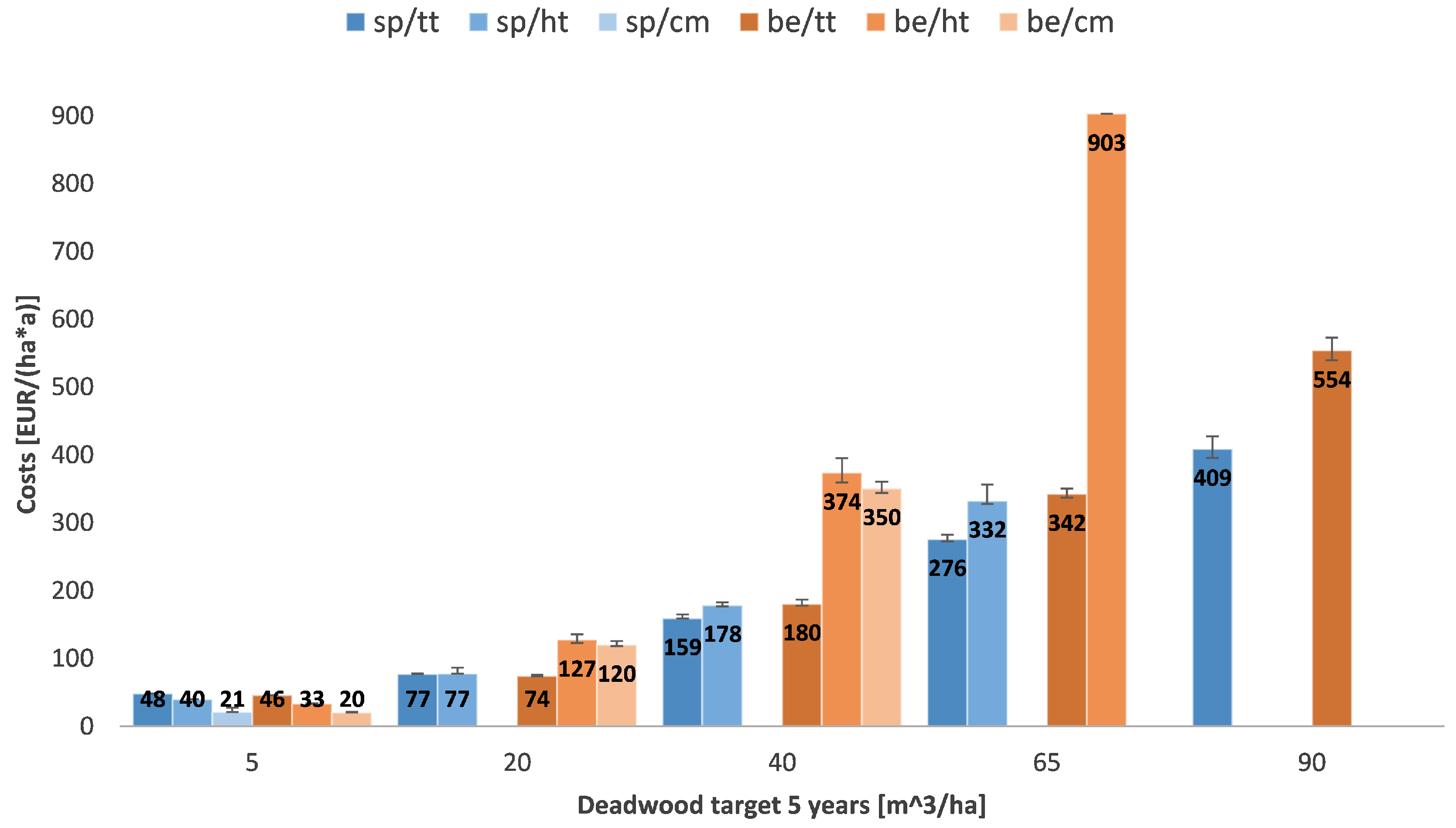
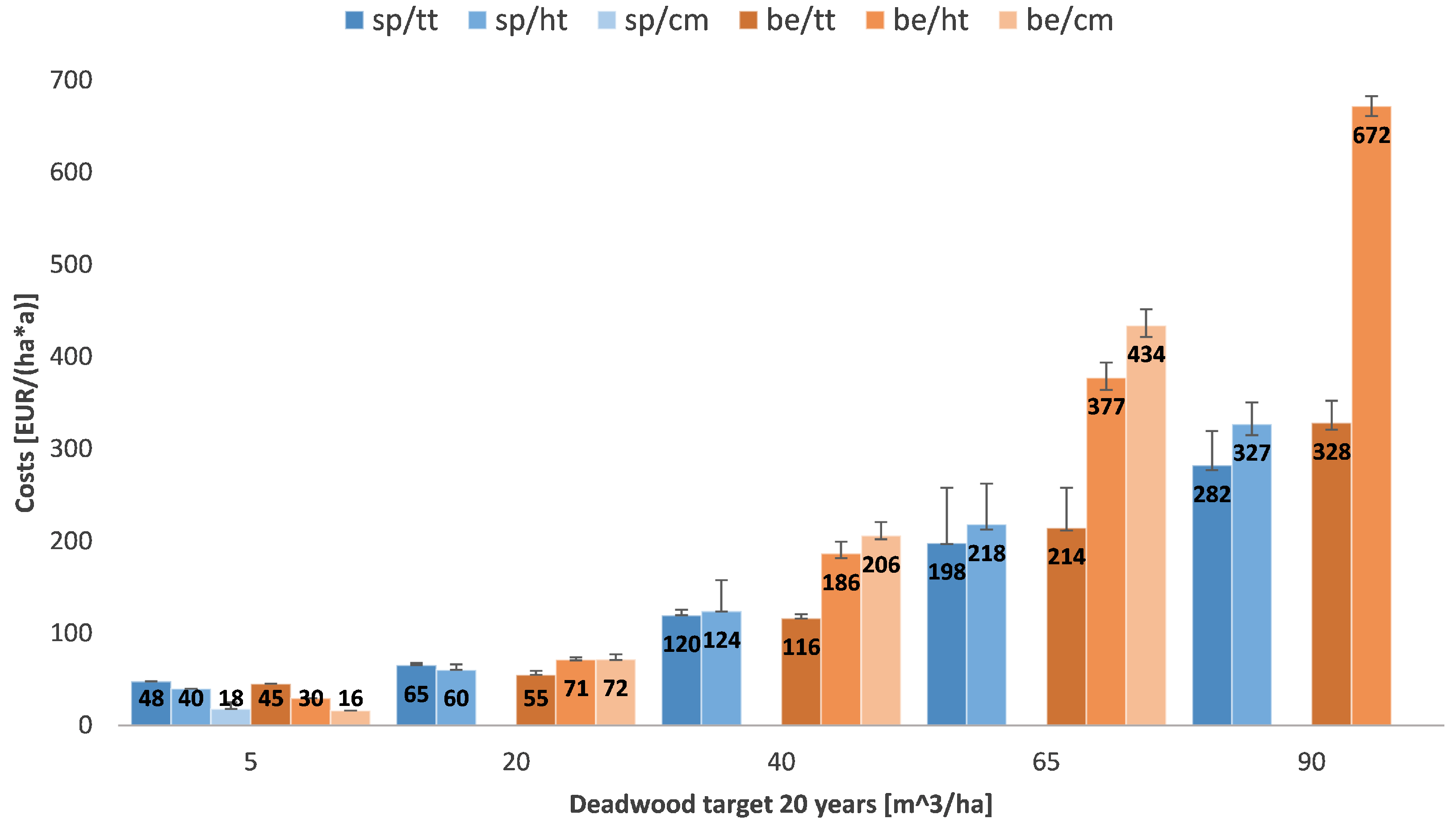
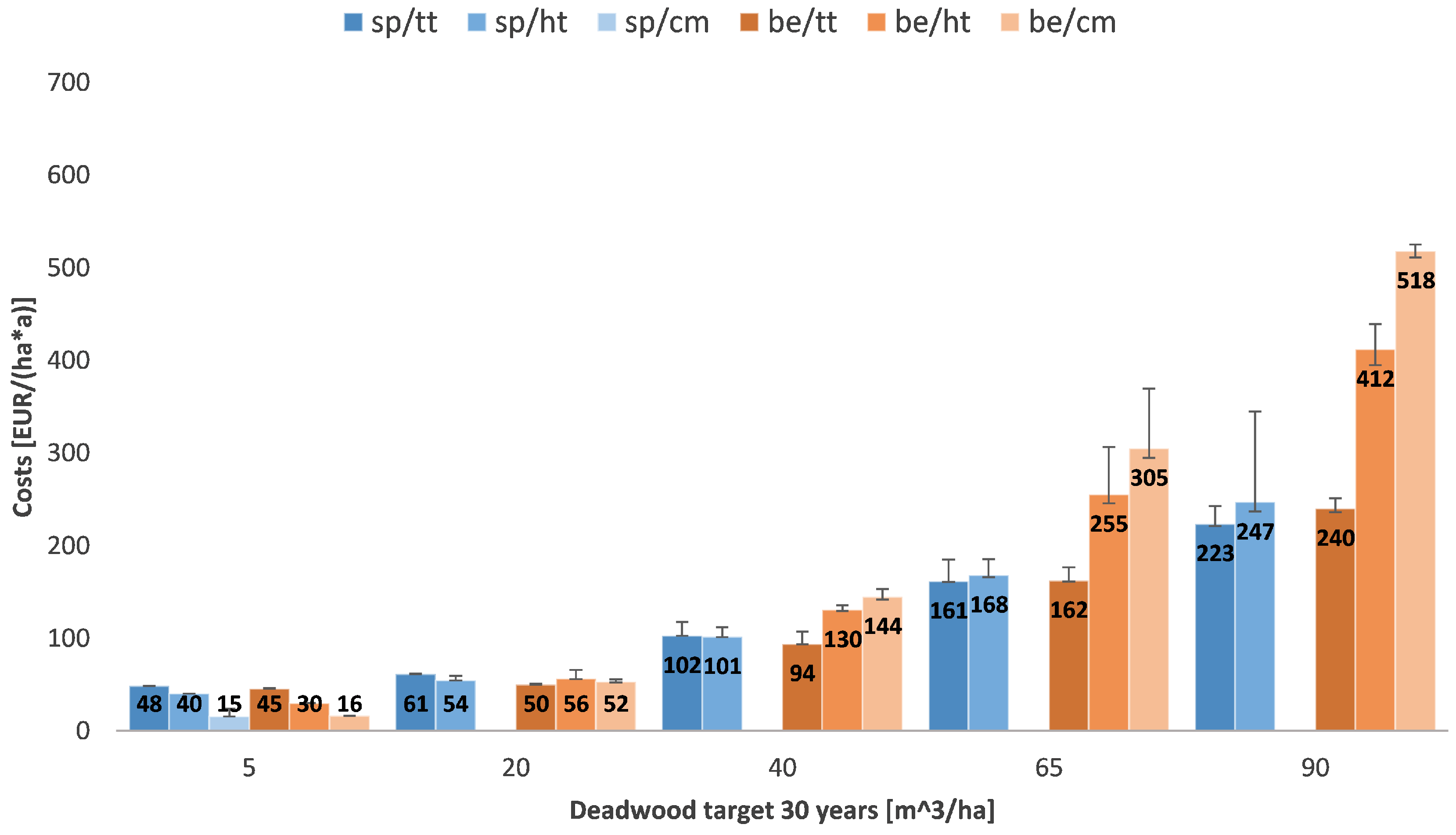
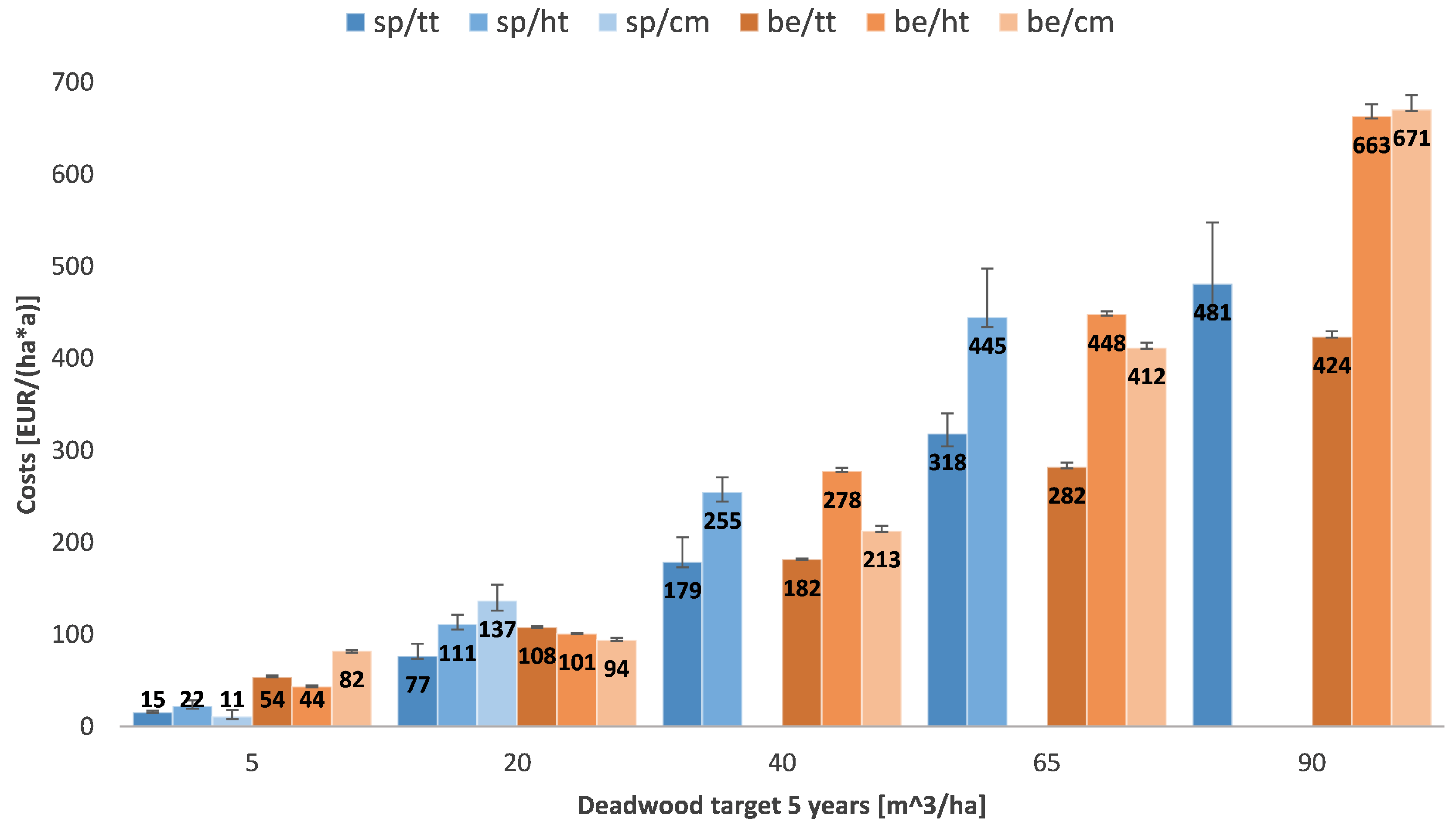
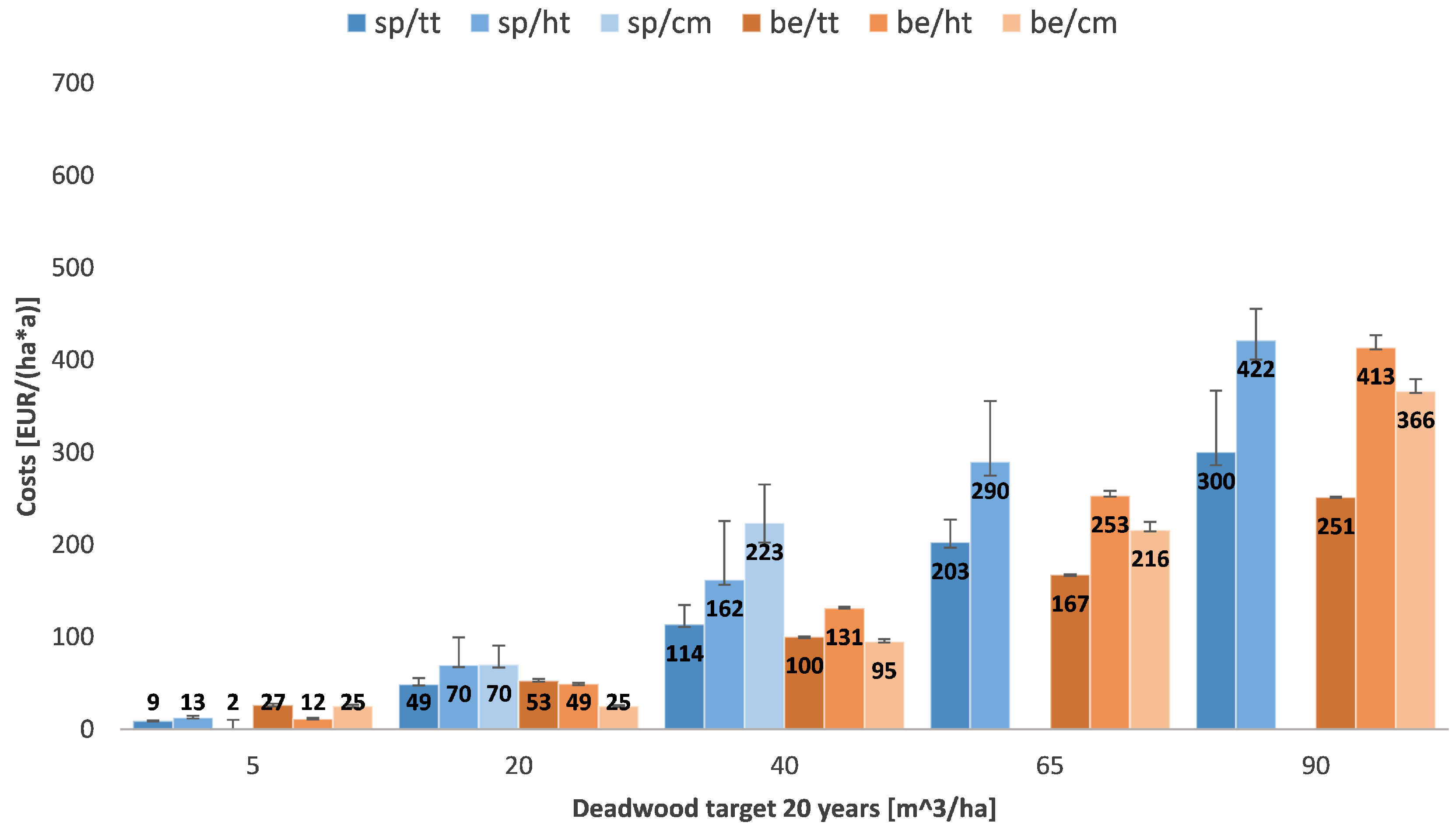
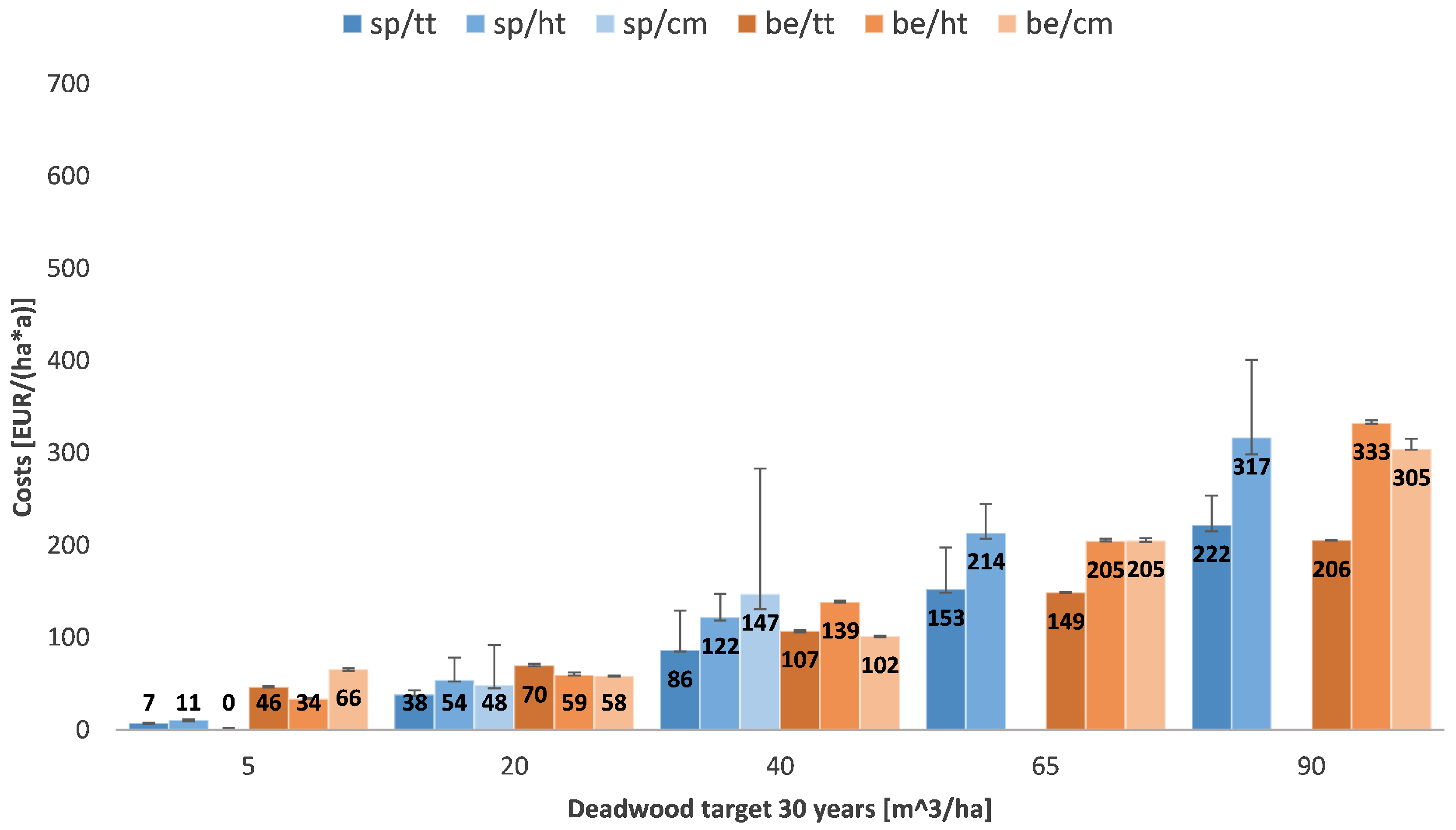
3.1. Analysing the Two Forest Enterprises Shows the General Tendencies

In order to analyse the effects of the deadwood scenarios on the different enterprises we simulated every possible combination with the two described data sets using the robust optimization. Starting with “Eichelberg”, the results for a time horizon of 5 years are shown in Figure 1. In the following, each single figure represents the costs per hectare (of beech or spruce stands) of the different scenarios for a specific time horizon, differentiated between deadwood target (x-axis), tree species and sorting strategy combination (colours of the bars), and the influence of the rate of segregation (symbolized as “error bars” showing the variation due to segregation from minimum to maximum). In general, the costs increase with an increasing deadwood target. The results for spruce show that reaching the target with crown material is only possible for a target of 5 ${\mathrm{m}}^3\mathrm{h}{\mathrm{a}}^{-1}$ being the option with the lowest costs. Using the total trees is the most expensive option and the heavy timber strategy is in between the other two. With a rising deadwood target, the relation between the total tree and the heavy timber approach shifts making the first more and more cost-effective until it remains the only option to achieve a total volume of 90 ${\mathrm{m}}^3\mathrm{h}{\mathrm{a}}^{-1}$. In the case of beech the pattern is similar. The crown material strategy can be applied up to 40 ${\mathrm{m}}^3\mathrm{h}{\mathrm{a}}^{-1}$ and is slightly more cost-effective than the heavy timber strategy. In general, the symbolized “error bars” show that a decreasing rate of segregation leads to an increase of the costs.

Table 4. Forest enterprise “Eichelberg”: Median costs and influence of the degree of segregation. The single strategies are abbreviated as shown in Table 3. Costs 1 shows the costs as the loss of annuity within the enterprise, while Costs 2 shows the costs related to the area of the individual tree species of the scenario. The Min. column shows the result for 100% segregation, the Max. column the result for 1% segregation.

Time Horizon	Strategy	Target	Costs 1	Costs 2	Min.	Max.
[years]		[m${}^3$ha${}^{-1}$]	[€ha${}^{-1}$a${}^{-1}$]	[€/ha/a]	[€ha${}^{-1}$a${}^{-1}$]	[€ha${}^{-1}$a${}^{-1}$]
5	sp/ht	5	22.6	39.6	39.6	39.7
		20	44.0	77.3	77.3	86.3
		40	101.7	178.4	176.5	182.5
		65	189.3	332.2	327.6	356.4
	sp/tt	5	27.4	48.0	48.0	48.0
		20	43.8	76.9	76.8	77.9
		40	90.6	159.0	158.6	164.8
		65	157.1	275.7	272.4	282.7
		90	232.8	408.7	395.5	427.2
	sp/cm	5	11.8	20.7	20.6	27.2
	be/ht	5	7.2	33.3	33.3	33.9
		20	27.7	127.4	122.8	135.5
		40	81.3	373.7	359.5	395.1
		65	196.4	902.9	902.9	902.9
	be/tt	5	9.9	45.5	45.5	45.5
		20	16.1	74.0	73.5	76.0
		40	39.2	180.3	177.8	186.6
		65	74.5	342.5	336.9	350.4
		90	120.5	553.9	539.8	572.7
	be/cm	5	4.4	20.5	20.4	21.4
		20	26.1	120.0	118.3	125.8
		40	76.2	350.5	344.2	360.5
20	sp/ht	5	22.6	39.6	39.6	39.7
		20	34.4	60.3	60.3	66.3
		40	70.6	123.9	123.4	157.6
		65	124.3	218.2	212.3	262.4
		90	186.3	327.0	315.0	350.5
	sp/tt	5	27.4	48.0	48.0	48.0
		20	37.2	65.4	65.3	67.7
		40	68.2	119.7	119.7	125.5
		65	112.7	197.9	196.6	257.8
		90	160.9	282.3	276.9	319.2
	sp/cm	5	10.2	17.8	17.8	25.2
	be/ht	5	6.5	29.7	29.7	29.7
		20	15.5	71.4	70.6	73.9
		40	40.5	186.4	181.5	199.2
		65	82.0	377.2	363.9	393.6
		90	146.1	671.8	660.9	682.7
	be/tt	5	9.9	45.4	45.4	45.4
		20	11.9	54.9	54.8	59.1
		40	25.3	116.4	115.8	120.8
		65	46.6	214.5	211.4	258.0
		90	71.4	328.5	320.6	352.2
	be/cm	5	3.5	15.9	15.9	16.1
		20	15.6	71.8	70.8	77.1
		40	44.8	205.8	201.8	220.7
30	sp/ht	5	22.6	39.6	39.5	39.6
		20	30.7	53.9	53.9	59.1
		40	57.7	101.2	101.0	111.6
		65	95.6	167.8	165.6	185.1
		90	140.5	246.6	236.6	344.4
	sp/tt	5	27.4	48.0	48.0	48.0
		20	34.7	61.0	60.9	61.3
		40	58.3	102.4	102.4	117.4
		65	91.9	161.3	160.6	184.8
		90	127.2	223.2	220.9	242.3
	sp/cm	5	8.6	15.2	15.1	23.5
	be/ht	5	6.5	29.7	29.7	29.7
		20	12.2	55.9	55.6	65.5
		40	28.4	130.5	129.0	135.2
		65	55.5	255.0	245.5	306.1
		90	89.5	411.7	394.8	438.9
	be/tt	5	9.9	45.4	45.4	45.4
		20	10.8	49.7	49.7	50.3
		40	20.4	93.7	93.3	106.7
		65	35.2	162.0	161.0	176.2
		90	52.2	239.8	235.9	250.8
	be/cm	5	3.5	15.9	15.9	16.1
		20	11.4	52.5	51.8	55.3
		40	31.4	144.4	141.5	153.0
		65	66.3	304.6	294.4	369.4
		90	112.6	517.8	510.9	524.7

shows that the median values are only slightly higher than the minimum values (corresponding to a segregation level of 100%). Consequently, very low rates of segregation (10% and less) lead to disproportionately high cost increases.

For a time horizon of 20 years, the costs as well as the differences between the single strategies increase with rising deadwood targets (Figure 2). For spruce the total tree approach becomes more cost-effective compared to the heavy timber strategy. The same pattern can be seen for beech, but with higher differences in between the sorting strategies. While using crown material of spruce is only possible for the 5 ${\mathrm{m}}^3\mathrm{h}{\mathrm{a}}^{-1}$ target, similar to the 5 year horizon, for beech this option will now be also available for the 65 ${\mathrm{m}}^3\mathrm{h}{\mathrm{a}}^{-1}$ target, although it is the strategy with the highest costs (434 $€\mathrm{h}{\mathrm{a}}^{-1}{\mathrm{a}}^{-1}$).

For the longest time horizon of 30 years, the pattern is similar to the results for 20 years (Figure 3). The differences between the sorting strategies are smaller but show similar rankings. Only in the case of a deadwood target of 40 ${\mathrm{m}}^3\mathrm{h}{\mathrm{a}}^{-1}$ the heavy timber strategy is now 1 $€\mathrm{h}{\mathrm{a}}^{-1}{\mathrm{a}}^{-1}$ on median average cheaper than the total tree approach. Comparing all three different time horizons one can see that the longer the time horizon to reach the deadwood target, the more cost-effective the target can be reached. As an extreme example, a target of 65 ${\mathrm{m}}^3\mathrm{h}{\mathrm{a}}^{-1}$ using heavy timber from beech costs 903 $€\mathrm{h}{\mathrm{a}}^{-1}{\mathrm{a}}^{-1}$, if it will be reached and maintained within 5 years, whereas the annual costs can be reduced to around one third ( 305 $€\mathrm{h}{\mathrm{a}}^{-1}{\mathrm{a}}^{-1}$), if the time horizon is stretched to 30 years. Similarly, a time horizon of 20 years has a severe cost-reducing effect ( 434 $€\mathrm{h}{\mathrm{a}}^{-1}{\mathrm{a}}^{-1}$). With low volume deadwood targets up to 20 ${\mathrm{m}}^3\mathrm{h}{\mathrm{a}}^{-1}$ the chosen time horizon is less important, especially for spruce, but even there, costs can be reduced by about 30% from 77 $€\mathrm{h}{\mathrm{a}}^{-1}{\mathrm{a}}^{-1}$to 54 $€\mathrm{h}{\mathrm{a}}^{-1}{\mathrm{a}}^{-1}$ for the heavy timber case.

Figure 4, Figure 5 and Figure 6 and

Table 5. Forest enterprise “Neureichenau”: Median costs and influence of the degree of segregation. The single strategies are abbreviated as shown in Table 3. Costs 1 shows the costs as the loss of annuity within the enterprise, while Costs 2 shows the costs related to the area of the individual tree species of the scenario. The Min. column shows the result for 100 % segregation, the Max. column the result for 1 % segregation.

Time Horizon	Strategy	Target	Costs 1	Costs 2	Min.	Max.
[years]		[m${}^{\mathbf{3}}$ha${}^{-\mathbf{1}}$]	[€ha${}^{-\mathbf{1}}$a${}^{-\mathbf{1}}$]	[€ha${}^{-\mathbf{1}}$a${}^{-\mathbf{1}}$]	[€ha${}^{-\mathbf{1}}$a${}^{-\mathbf{1}}$]	[€ha${}^{-\mathbf{1}}$a${}^{-\mathbf{1}}$]
5	sp/ht	5	18.9	22.4	19.6	28.8
		20	93.9	111.1	105.5	121.3
		40	215.4	254.8	244.3	270.7
		65	376.2	445.1	434.1	497.7
	sp/tt	5	13.0	15.4	14.6	17.3
		20	65.0	76.9	73.6	90.0
		40	151.3	179.1	173.1	205.8
		65	269.1	318.4	304.5	340.5
		90	406.7	481.2	447.8	547.7
	sp/cm	5	9.4	11.2	8.2	17.9
		20	115.8	137.0	125.8	154.2
	be/ht	5	1.0	43.7	42.9	44.7
		20	2.4	101.1	100.6	101.6
		40	6.6	277.7	276.5	281.0
		65	10.7	448.1	446.3	451.3
		90	15.9	663.2	660.9	676.0
	be/tt	5	1.3	53.9	53.5	55.8
		20	2.6	108.1	106.8	109.1
		40	4.3	181.8	181.0	182.6
		65	6.7	282.2	280.8	286.9
		90	10.1	423.9	422.6	429.5
	be/cm	5	2.0	82.4	80.3	83.2
		20	2.3	94.2	92.9	96.2
		40	5.1	212.6	211.7	218.0
		65	9.8	411.7	410.5	417.1
		90	16.0	670.8	668.9	686.0
20	sp/ht	5	11.0	13.0	11.8	14.7
		20	58.9	69.6	67.5	99.5
		40	137.1	162.3	156.7	225.8
		65	244.9	289.8	274.7	355.5
		90	356.3	421.5	400.6	455.5
	sp/tt	5	7.8	9.2	8.6	9.6
		20	41.1	48.7	47.6	55.6
		40	96.2	113.8	110.8	134.8
		65	171.2	202.6	196.7	227.1
		90	253.9	300.4	286.0	366.8
	sp/cm	5	1.4	1.7	−2.0	10.2
		20	59.4	70.2	67.1	90.7
		40	188.9	223.5	202.5	265.2
	be/ht	5	0.3	11.5	10.6	12.4
		20	1.2	49.3	48.2	50.4
		40	3.1	131.4	130.6	132.8
		65	6.1	253.2	252.2	258.2
		90	9.9	413.5	411.5	427.0
	be/tt	5	0.6	26.5	25.0	27.9
		20	1.3	52.7	51.5	54.4
		40	2.4	100.3	98.9	100.6
		65	4.0	167.5	166.2	167.9
		90	6.0	251.2	250.7	252.2
	be/cm	5	0.6	25.2	23.7	26.6
		20	0.6	25.3	24.4	26.5
		40	2.3	95.0	94.2	97.6
		65	5.2	215.9	214.5	224.5
		90	8.8	366.3	364.6	379.6
30	sp/ht	5	9.0	10.6	9.0	11.2
		20	45.6	54.0	52.4	78.3
		40	103.2	122.0	118.4	147.4
		65	180.6	213.7	207.0	244.7
		90	267.6	316.6	298.4	401.0
	sp/tt	5	6.2	7.3	6.2	7.8
		20	32.5	38.4	36.4	42.8
		40	72.9	86.2	84.7	129.3
		65	129.0	152.6	148.5	197.5
		90	187.6	222.0	215.2	253.8
	sp/cm	5	0.2	0.2	-2.0	1.7
		20	41.0	48.5	44.9	91.9
		40	124.5	147.3	130.4	283.3
	be/ht	5	0.8	33.6	33.1	34.6
		20	1.4	59.5	58.7	62.1
		40	3.3	138.7	137.9	140.0
		65	4.9	204.8	204.0	206.9
		90	8.0	332.6	331.6	335.6
	be/tt	5	1.1	46.3	45.8	47.4
		20	1.7	69.8	68.6	71.8
		40	2.6	107.2	105.8	107.8
		65	3.6	148.8	148.1	149.2
		90	4.9	205.5	205.1	206.1
	be/cm	5	1.6	65.9	63.9	66.7
		20	1.4	58.5	57.8	58.8
		40	2.4	101.5	100.3	101.9
		65	4.9	205.2	203.8	207.6
		90	7.3	304.7	303.5	315.5

show the results for “Neureichenau” in the same structure as explained for the “Eichelberg” case. The overall pattern of the results is the same so we focus on the differences between the two cases. Comparing the two series of figures one can see some differences: There are more options for the crown material strategies especially with beech in “Neureichenau”. The beech strategies tend to be cheaper than in the “Eichelberg” case whereas the spruce strategies are more expensive. While in the 5 year scenarios both spruce and beech scenarios produce similar costs, beech tends to get more cost-effective in the long run compared to spruce (see Figure 5 and Figure 6). Also, the crown material strategy for beech remains cheaper than the heavy timber strategy in almost all cases (exceptions are the 90 ${\mathrm{m}}^3\mathrm{h}{\mathrm{a}}^{-1}$ deadwood target within 5 years and all the 5 ${\mathrm{m}}^3\mathrm{h}{\mathrm{a}}^{-1}$ scenarios) whereas in the “Eichelberg” case this was true only for the 5 year time horizon.

For all results one has to keep in mind, that the presented amounts are volumes without bark and also without accounting for any supply of deadwood from stumps or root volumes.

Overall we can derive the following tendencies:

• All scenarios

  (a)

  The higher the desired deadwood amount is set, the higher are the linked costs.

  (b)

  The longer the time horizon to reach the desired deadwood amount is chosen, the more cost-effective the target that can be reached.

  (c)

  The actual costs depend on the stand structure of the forest enterprise.

  (d)

  There is no clear ranking between the spruce and the beech scenarios.

  (e)

  A segregative approach leads to lower costs than the integrative patterns.

• Spruce scenarios

  (a)

  Starting from deadwood amounts of 20 ${\mathrm{m}}^3\mathrm{h}{\mathrm{a}}^{-1}$ and more, the crown material option is more expensive than the heavy timber strategy. The total tree approach is the most cost-effective. For low deadwood targets (5 ${\mathrm{m}}^3\mathrm{h}{\mathrm{a}}^{-1}$) the crown material option is the cheapest.

  (b)

  Within a larger forest enterprise more deadwood objectives can be reached with crown material.

• Beech scenarios

  (a)

  In most scenarios the total tree strategy has the biggest cost advantage.

  (b)

  From deadwood amounts of 40 ${\mathrm{m}}^3\mathrm{h}{\mathrm{a}}^{-1}$ and more, the heavy timber strategy is more cost-intensive than the use of total trees. (In the case of “Eichelberg” this is already true for a deadwood target of 20 ${\mathrm{m}}^3\mathrm{h}{\mathrm{a}}^{-1}$.)

  (c)

  The ranking between the crown material and the heavy timber strategy depends on the enterprise.

3.2. Comparison of the Robust Model with the Stochastic Approach Reveals Its Stability

These returns were then used to calculate the average annuity according to the solution of the stochastic model as well as the robust model.

Table 6. Mean annuities and standard deviations of the stochastic model and the robust model derived from 100 Monte Carlo simulations of the uncertain possible revenues of each stand. Random values are chosen from the part of the uncertainty space that includes negative derivations from the nominal value. For abbreviations see Table 3.

Time Horizon	Strategy	Target	Stochastic		Robust		Diff.
			Mean	Std.dev.	Mean	Std.dev.	Mean	Std.dev.
[years]		[m${}^3$ha${}^{-1}$]	[€ha${}^{-1}$a${}^{-1}$]	[€ha${}^{-1}$a${}^{-1}$]	[€ha${}^{-1}$a${}^{-1}$]	[€ha${}^{-1}$a${}^{-1}$]	[%]	[%]
baseline		0	598.0	67.4	583.1	54.1	−2.5	−19.7
5	sp/tt	20	561.8	70.6	547.7	60.5	−2.5	−14.4
		65	420.6	43.4	413.4	39.1	−1.7	−9.8
	be/tt	20	579.8	64.8	568.5	53.3	−1.9	−17.7
		65	515.7	49.1	503.9	36.2	−2.3	−26.3
20	sp/tt	20	551.5	60.2	542.1	54.5	−1.7	−9.5
		65	469.9	49.7	460.8	40.8	−1.9	−17.9
	be/tt	20	581.9	65.2	569.2	55.7	−2.2	−14.6
		65	552.0	53.5	538.0	38.6	−2.5	−27.8
30	sp/tt	20	562.7	64.1	546.8	52.4	−2.8	−18.2
		65	496.1	62.2	480.2	45.5	−3.2	−26.8
	be/tt	20	586.3	59.7	573.7	53.7	−2.2	−10.1
		65	551.5	64.5	537.9	49.3	−2.5	−23.7
Mean							−2.3	−18.2

shows the results for a representative selection of the different deadwood scenarios. For all chosen deadwood scenarios, the robust solutions achieve lower standard deviations (reductions range from 9.5% to 27.8%, on average 18.2%). This robustness towards uncertainty is accompanied by a slight reduction of the overall expected annuities. The relative reductions of the expected annuities are between 1.7% and 3.2% (on average 2.3%). This shows that the robust solution considerably reduces the uncertainties in the objective function with only moderate reduction of the expected mean.

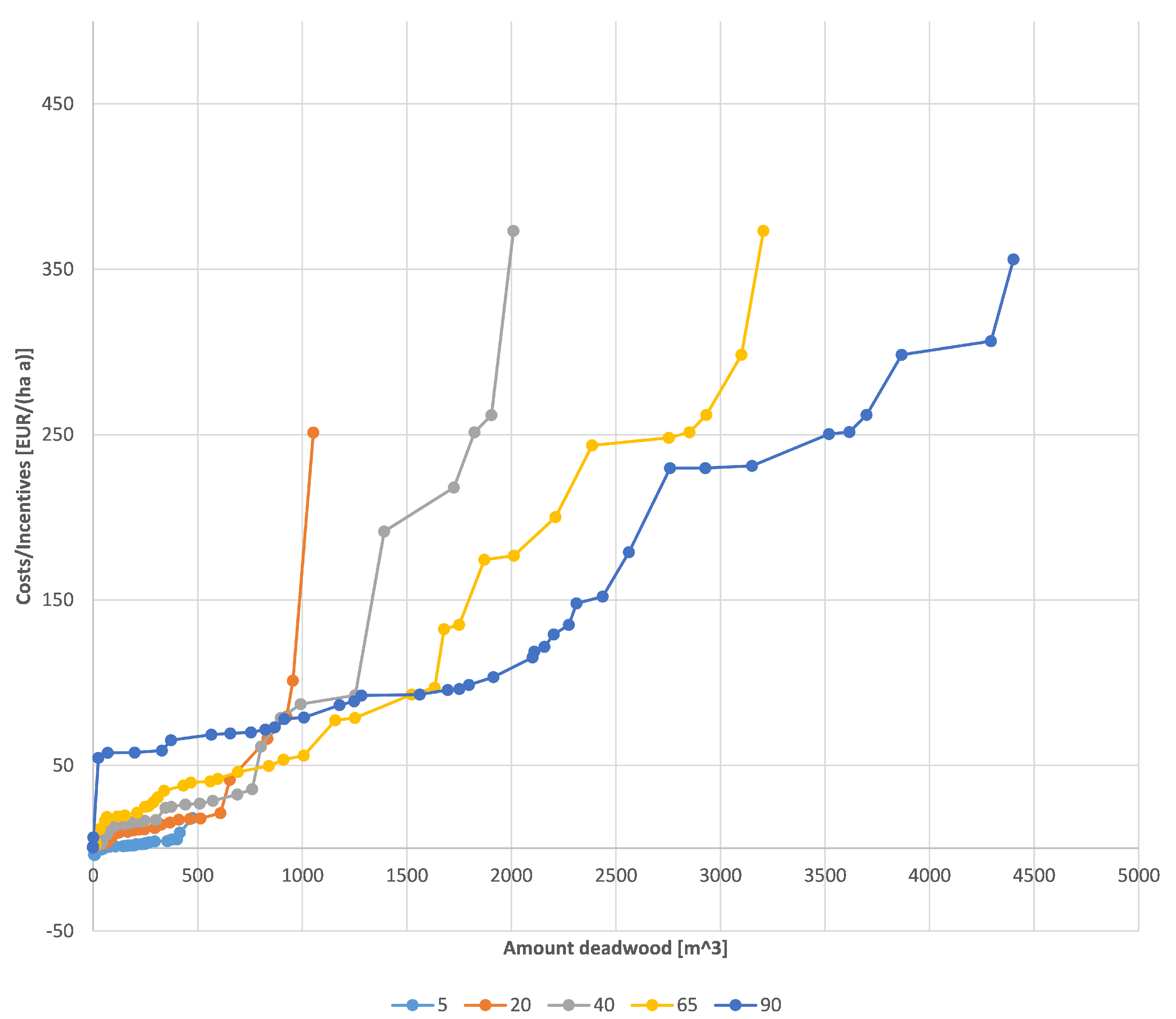
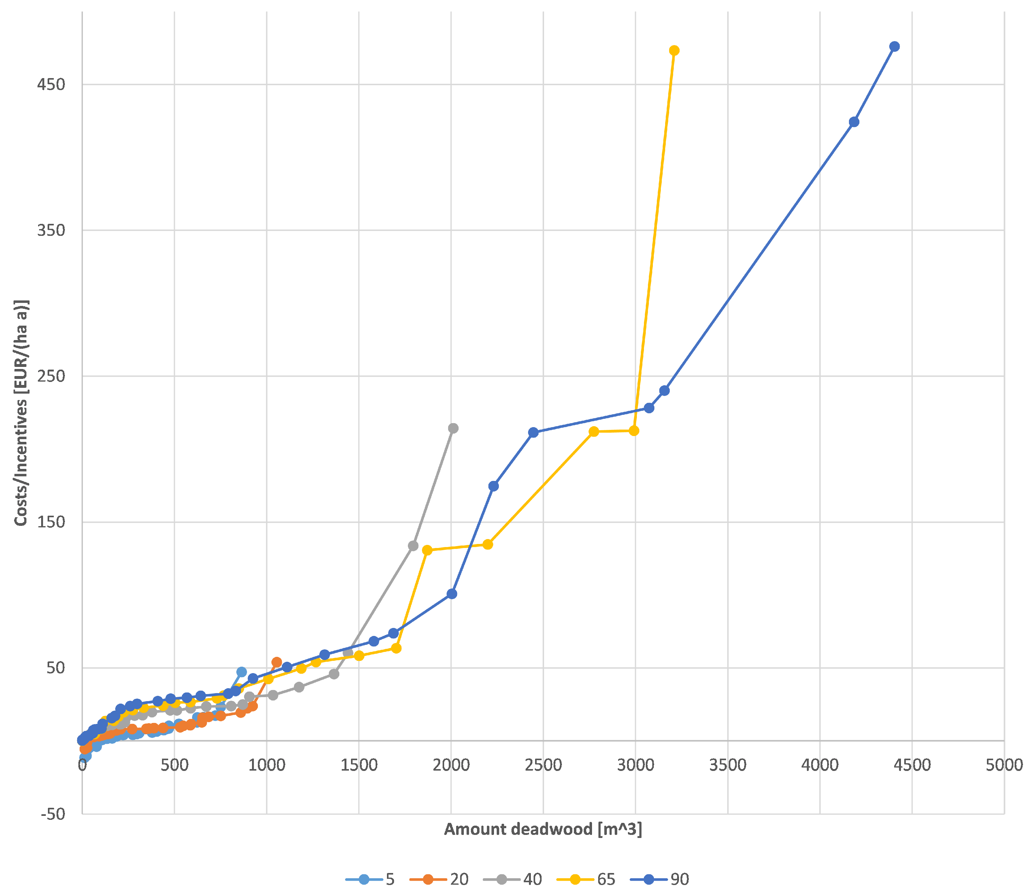
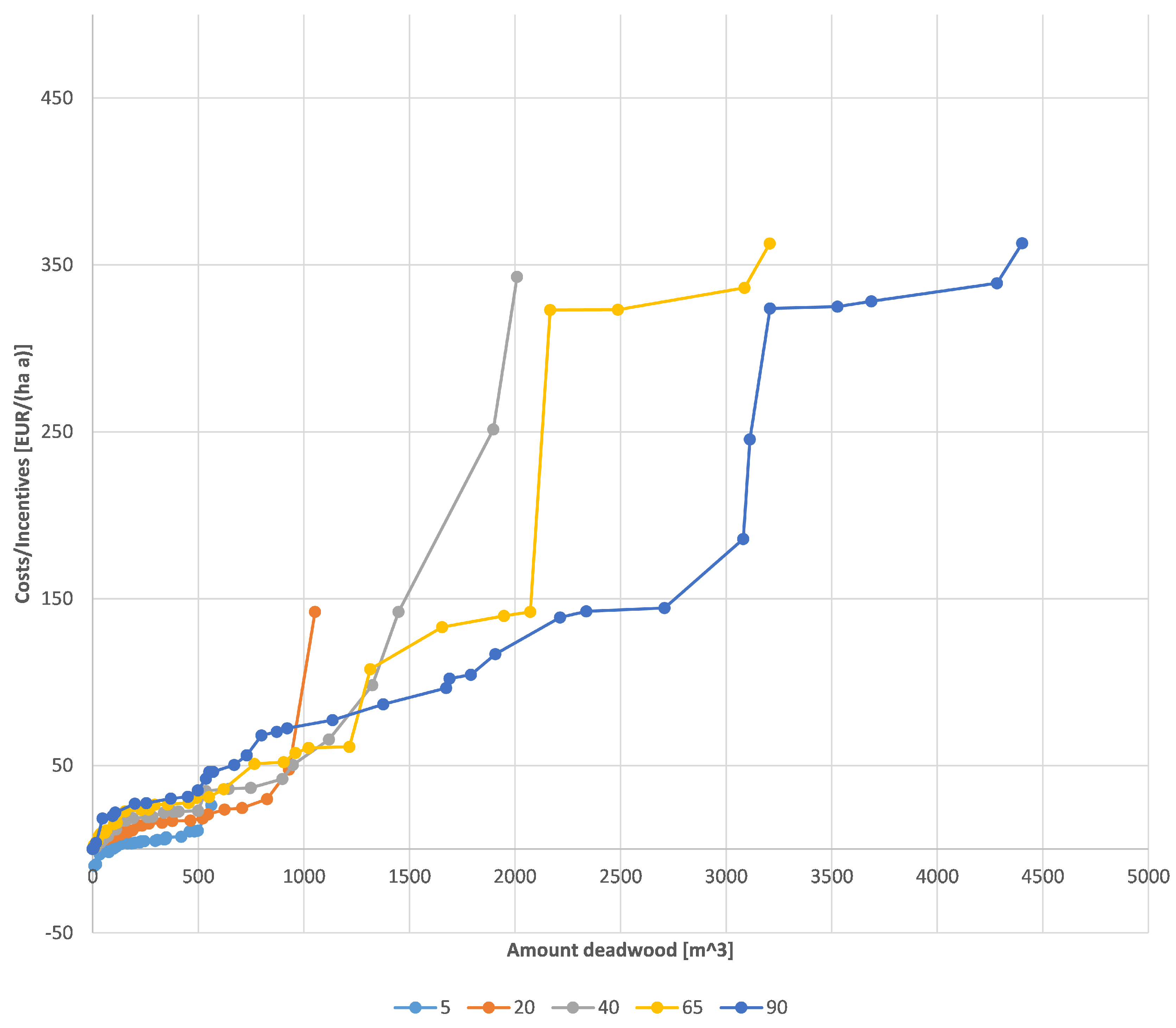
3.3. Analysis of Deadwood Supply Derives Effective Strategy Combinations

If we investigate the structure of the individual costs of the different forest stands we can derive supply curves that can help to support effective market behaviour of single forest enterprises. As an example, we used the data of “Eichelberg” of the deadwood scenarios with beech for the time horizon of 30 years. Figure 7 shows the individual costs for using crown material induced in the single forest stands (again as losses of annuities) related to the amount of deadwood that can be supplied by these stands. In doing so we get individual supply curves for the different strategies of deadwood densities from 5 ${\mathrm{m}}^3\mathrm{h}{\mathrm{a}}^{-1}$ to 90 ${\mathrm{m}}^3\mathrm{h}{\mathrm{a}}^{-1}$. As a higher deadwood density within the given area of beech stands can reach higher absolute amounts of deadwood, the curves end at different maximum levels of deadwood (from 475 ${\mathrm{m}}^3$ to 4402 ${\mathrm{m}}^3$). A second pattern is that high density strategies tend to be more cost-effective with higher absolute amounts of deadwood (above 1700 ${\mathrm{m}}^3$), while low-density strategies are more effective in maintaining low absolute volumes of deadwood (below 700 ${\mathrm{m}}^3$). For intermediate levels of 700 ${\mathrm{m}}^3$ to 1700 ${\mathrm{m}}^3$ the effectiveness of the different strategies is quite similar.

The supply curve shows that the forest owner can provide for example up to 3500 ${\mathrm{m}}^3$ of deadwood using a strategy of maintaining 90 ${\mathrm{m}}^3\mathrm{h}{\mathrm{a}}^{-1}$, if he will get paid 250 $€\mathrm{h}{\mathrm{a}}^{-1}{\mathrm{a}}^{-1}$ for that service. Would he use a strategy of providing a level of 20 ${\mathrm{m}}^3\mathrm{h}{\mathrm{a}}^{-1}$, he could maintain only 1050 ${\mathrm{m}}^3$ – with the same costs. If the incentive will be at 35 $€\mathrm{h}{\mathrm{a}}^{-1}{\mathrm{a}}^{-1}$, he can provide 760 ${\mathrm{m}}^3$ with a density of 40 ${\mathrm{m}}^3\mathrm{h}{\mathrm{a}}^{-1}$. However, only 340 ${\mathrm{m}}^3$ if he is for example enforced by incentive regulations to use a strategy of 65 ${\mathrm{m}}^3\mathrm{h}{\mathrm{a}}^{-1}$.

A more balanced structure can be seen in Figure 8 for using the total tree strategies. Here, the different density approaches do not differ much and the shifting in cost-effectiveness is gradually from 5 ${\mathrm{m}}^3\mathrm{h}{\mathrm{a}}^{-1}$ to 90 ${\mathrm{m}}^3\mathrm{h}{\mathrm{a}}^{-1}$ scenarios with increasing absolute deadwood amounts. Figure 9 shows the results for the heavy timber approaches. This pattern is more similar to the results for using crown material.

4. Discussion

4.1. Robust and Stochastic Approach Lead to Similar Results

As our approach includes deadwood targets in a risk-considering optimization tool on enterprise level, the tool decides about the types of assortments, stands, and the time horizon to achieve the desired deadwood targets. This enables the possibility to compare the effects of several optimised strategies. To model the deadwood amount, we use an exponential decay function. Another approach would be the use of linear decay models ([31], for an overview cf. Mackensen and Bauhus [22]). The ostensible advantage of linear models is that they seem to explain data from measurements of deadwood amounts in forests quite well. In contrast, exponential models lead to relative long decay times that seem not be confirmed by experimental data. However, experimental data often underestimate small scale fragments of deadwood as they are easily overseen on the forest floor making exponential models yet the better choice.

Furthermore, we used a stochastic as well as a robust optimization approach for the investigation. The results showed that the robust approach and the stochastic approach deliver similar results. As described in the method section the robust optimization skips the information of the functional distribution of the assumed uncertainties. Consequently, its advantage is that less data are needed to collect or assume, making it an easier method to apply in forestry where data collection is typically very time and money consuming. However, the results of Table 6 show that the stability against random realizations of the unknown returns is raised by the robust solution. Comparing the values of the returns between the both optimization approaches shows that the robust means are generally below the stochastic means but closer to the individual baseline. Therefore, the robust system leads to more stable results over all deadwood scenarios.

The derived costs are given as annuity losses on the enterprise level. This implies that the results are valid for enterprises consisting of pure stands of the individual species. To relate them to a real enterprise, the figures have to be reduced by the actual proportion of beech or spruce stands. If there are different deadwood objectives planned for different stand classes, the costs have to be reduced to the area of that particular stand class (for example if one wants to achieve a deadwood target of 40 ${\mathrm{m}}^3\mathrm{h}{\mathrm{a}}^{-1}$ in beech stands older than 140 years only, cf. BaySF [76]).

4.2. Some Results Are Comparable to Other Studies

The basic patterns of the results are reasonable. Higher costs with increasing deadwood amounts have been shown by other studies [43]. The authors present costs as net present values of 301 $€\mathrm{h}{\mathrm{a}}^{-1}$ for 5 ${\mathrm{m}}^3\mathrm{h}{\mathrm{a}}^{-1}$ of deadwood to around 2034 $€\mathrm{h}{\mathrm{a}}^{-1}$ for 48 ${\mathrm{m}}^3\mathrm{h}{\mathrm{a}}^{-1}$ of deadwood. The equivalent annuities are 9 $€\mathrm{h}{\mathrm{a}}^{-1}{\mathrm{a}}^{-1}$ and 59 $€\mathrm{h}{\mathrm{a}}^{-1}{\mathrm{a}}^{-1}$. While the costs at the low end correspond to our results, the higher costs differ ( 59 $€\mathrm{h}{\mathrm{a}}^{-1}{\mathrm{a}}^{-1}$ compared for example to 179 $€\mathrm{h}{\mathrm{a}}^{-1}{\mathrm{a}}^{-1}$ for 40 ${\mathrm{m}}^3\mathrm{h}{\mathrm{a}}^{-1}$ of spruce deadwood within 5 years in “Neureichenau”). This is caused by the different assumptions about the timber prices and the different growth conditions. While Santaniello et al. [43] calculate with average prices of $43.84$$€{\mathrm{m}}^{-3}$ for spruce, we assumed 83 $€{\mathrm{m}}^{-3}$ for sawlogs of diameter class 20 cm to 24 cm and 50 $€{\mathrm{m}}^{-3}$ for pulpwood. Furthermore, their study region is a low-productivity forest in Scandinavia while our results are derived from high-productivity forests in Central Europe. Additionally, our study integrates the dynamics of the deadwood decay as we derived costs for maintaining a certain amount of deadwood instead of providing it once in time.

Wikström and Eriksson [38] calculated relative net present value losses of up to about 5%, 10% and 25% for deadwood amounts of 10 ${\mathrm{m}}^3\mathrm{h}{\mathrm{a}}^{-1}$, 20 ${\mathrm{m}}^3\mathrm{h}{\mathrm{a}}^{-1}$ and 40 ${\mathrm{m}}^3\mathrm{h}{\mathrm{a}}^{-1}$, respectively, in single stands that are mixed of birch and Norway spruce of low diameters at breast height (average between 8 cm and 11 cm). Their results are not comparable with ours as they defined these deadwood amounts as the total sum over a time horizon of 100 years. Furthermore, their model did not include any decay functions.

Tikkanen et al. [41] derived net present values of 62 $€{\mathrm{m}}^{-3}$ for providing spruce deadwood. Assuming a deadwood objective of 40 ${\mathrm{m}}^3\mathrm{h}{\mathrm{a}}^{-1}$, this is equivalent to 90 $€\mathrm{h}{\mathrm{a}}^{-1}{\mathrm{a}}^{-1}$. Their simulation is based on stands with an age from between 30 to 40 years, so the results are comparable to our deadwood target within 30 years. In that case, we derived comparable 86 $€\mathrm{h}{\mathrm{a}}^{-1}{\mathrm{a}}^{-1}$ in “Neureichenau” and 102 $€\mathrm{h}{\mathrm{a}}^{-1}{\mathrm{a}}^{-1}$ in “Eichelberg” for the total tree strategy.

Jonsson et al. [40] present costs for different deadwood treatments in Sweden. They derived net present values of around 219 $€\mathrm{h}{\mathrm{a}}^{-1}$ (2191 SEK ha${}^{-1}$) for an increase of $6.63$ ${\mathrm{m}}^3\mathrm{h}{\mathrm{a}}^{-1}$ of spruce deadwood assuming a retention area of 5% in stands in Southern Sweden. This is equivalent to about 8 $€\mathrm{h}{\mathrm{a}}^{-1}{\mathrm{a}}^{-1}$ and, therefore, comparable to our findings for the 5 ${\mathrm{m}}^3\mathrm{h}{\mathrm{a}}^{-1}$ scenarios in the large enterprise “Neureichenau”.

Jacobsen et al. [42] derived a net present value reduction of up to 10% due to deadwood management in NATURA 2000 areas. Compared with our results for deadwood objectives in “Eichelberg” within 5 years, this is true for objectives up to 20 ${\mathrm{m}}^3\mathrm{h}{\mathrm{a}}^{-1}$ of spruce deadwood and up to 40 ${\mathrm{m}}^3\mathrm{h}{\mathrm{a}}^{-1}$ of beech deadwood.

Ekvall et al. [44] derived an average net present value of 15 $€{\mathrm{m}}^{-3}$ (146.80 SEK m${}^{-3}$) for a mix of different deadwood strategies on enterprise level using a risk-free linear programming model. On average, their scenario adds 15 ${\mathrm{m}}^3\mathrm{h}{\mathrm{a}}^{-1}$ of deadwood. The calculated costs are equivalent to only $0.54$$€\mathrm{h}{\mathrm{a}}^{-1}{\mathrm{a}}^{-1}$. This result can be explained by their approach of combining different deadwood strategies to achieve the additional deadwood amount, and by starting with an initial volume of 20 ${\mathrm{m}}^3\mathrm{h}{\mathrm{a}}^{-1}$.

4.3. Other Results Reveal Additional Important Aspects of Deadwood Management

Another relation exists between sinking costs and longer time horizons. For example, a deadwood target of 20 ${\mathrm{m}}^3\mathrm{h}{\mathrm{a}}^{-1}$ within 5 years leads almost to the same costs as a target of 40 ${\mathrm{m}}^3\mathrm{h}{\mathrm{a}}^{-1}$ within 30 years. This effect is caused by the increasing flexibility to achieve the deadwood target within a longer time range and the discount effect. Reaching and maintaining a deadwood objective farer in the future affects the decision maker today much less than a short time goal. This result shows, that not only the actual deadwood amounts have to be chosen carefully, but also in which time period these targets must be reached. This aspect has yet rarely been investigated.

Increasing the rate of segregation leads to more cost-effective solutions, as the deadwood amounts can be selected more effective from stands of the most appropriate timber dimensions and age. The more integrative approaches imply an additional restriction, as they force to distribute the deadwood provision into stands less suitable for that purpose – in economic terms. Another aspect that has not been investigated so far.

Besides these general findings, the results show that they are influenced by the actual state of the forests in the given enterprise. One aspect is the relationship between the costs of using either beech or spruce. In the case of “Eichelberg” spruce is the cheaper solution, while in the case of “Neureichenau” the costs are equal or slightly lower for beech. An explanation is the age distribution of the stands. For “Eichelberg” the mean age of beech stands is 59 years in the first simulation period, with a range from 24 to 92 years. In the case of “Neureichenau” the mean age is at 79 years, with a range from 34 to 173 years. Therefore, “Neureichenau” starts with already more mature stands, implying the following aspects: The average overall volume of the beech stands is higher, as well as the mean volume of the trees. The older trees have bigger crowns and provide more crown material in total as well as per tree. Therefore, the costs of the crown material strategy will decrease, as bigger amounts can be provided by cutting down fewer trees which can be selected from a bigger population. Therefore, the cost advantage of using low-valued assortments joined to economically mature trees with valuable roundwood segments comes into effect without being foiled by the disadvantage of needing a lot of trees to provide the overall deadwood volume. This explains, why the crown material strategy shows reduced costs in the case of the older beech stands in “Neureichenau”, compared to the heavy timber strategy, and compared to the younger stands in “Eichelberg”.

In general, the results for the crown material strategies might be overestimated, due to the tree models available. As there is no model or sorting algorithm known to us, that simulate side branches with large diameters, that are common for older beech crowns, the overall amount of crown material in real forests may be higher than simulated. To compensate this effect to some extent, we increased the maximum diameter of logs for beech that are considered as being part of the crown (cf. Section 1.2). Despite this adjustment, there may be situations in forest enterprises with mainly old growth beech stands, where crown material strategies will be the most economic choice.

The relation of the costs for the spruce strategies can be explained the same way. The mean age of the stands in “Eichelberg” is 74 years (ranging from 44 to 91 years) and 62 years for “Neureichenau” (ranging from 11 to 146 years). The bigger amount of non-mature spruce stands increases the costs of providing deadwood from these stands—especially for the higher deadwood targets—despite the large overall area of spruce stands (13,288 ha).

The pattern within the spruce strategies can be explained by timber prices and timber volumes. Using crown material has the advantage of being a cheap option. As these amounts may only be used as fuelwood, they cannot be sold for a high price. The disadvantage of this strategy is, that a single softwood tree does not provide a large volume of crown material, due to its natural habit. Therefore, the advantage of being a cheap option can be used only for low deadwood targets up to 5 ${\mathrm{m}}^3\mathrm{h}{\mathrm{a}}^{-1}$. Higher volumes can only be reached for the sake of high costs that follow from cutting non-mature trees. The results show that in the case of “Eichelberg” the provision of heavy timber is cheaper than that of total trees for smaller targets up to 20 ${\mathrm{m}}^3\mathrm{h}{\mathrm{a}}^{-1}$. This can be explained again with the structure of the timber prices and the age distribution of the spruce stands. The high amount of mature stands makes it cheaper to use some heavy timber trunks of bad quality for the provision of low deadwood amounts and selling the remaining better assortments of the tree than using the total tree for deadwood. This is a special case for “Eichelberg” and no general rule as this pattern cannot be seen in the case of “Neureichenau”.

In a similar way, the more diverse pattern of the beech strategies are explained. The higher timber volume of beech crowns provides the cost advantage of this option, as long as there are enough beech stands to use flexibly from. In that combination, this option can be more cost-effective than the heavy timber approach. For targets of 20 ${\mathrm{m}}^3\mathrm{h}{\mathrm{a}}^{-1}$ and 40 ${\mathrm{m}}^3\mathrm{h}{\mathrm{a}}^{-1}$ within 20 years or more, it is the cheapest method. This advantage cannot be realized, if there are not enough mature beech stands available, like in the case of “Eichelberg”, where only 48 $\mathrm{h}\mathrm{a}$ of beech stands with an average age of 59 years exist.

The results for deadwood amounts of 5 ${\mathrm{m}}^3$ ${\mathrm{h}\mathrm{a}}^{\mathrm{-1}}$ with beech in “Neureichenau” show an anomaly, as the crown material strategies have the highest costs. This can be explained with the contradicting mechanisms mentioned above. In this case, the low overall deadwood volume can be reached by using total trees or heavy timber logs. Contrary to the other scenarios, the limitation of using only crown material is a more severe restriction than the heavy timber strategy. In the first simulation period, in which the deadwood target fully applies, $7.0$ $\mathrm{h}\mathrm{a}$ are necessary to build up the deadwood from crown material, while the heavy timber strategy uses $4.0$ $\mathrm{h}\mathrm{a}$ and the total tree option $3.2$ $\mathrm{h}\mathrm{a}$ of beech stands. While the model accounts for the selling of the remaining assortments, almost doubling the size of the deadwood area causes heavy losses in selling non-mature timber.

4.4. Supply Analysis as A Management Approach to React on Market Prices

The results of the supply analysis show, that the different deadwood densities change their ranks of cost-effectiveness. This depends on the overall absolute deadwood amount, that will be maintained in the forest enterprise. Furthermore, as the Figure 7, Figure 8 and Figure 9 show supply curves of the individual forest enterprise, it is possible to derive an individual producer surplus from these graphs, if the costs on the y-axis are interpreted as the market prices of deadwood (for example, if there are public incentives available). The producer surplus is identical to the area between a parallel to the x-axis at the level of the market price and the supply curve. This means, that the surplus is maximised by shifting the supply curve to the right and/or the bottom of the diagram. As the actual supply curves intersect with each other, a mixture of different deadwood targets is the most economic way to react on a given market price for deadwood (or an incentive). The new, combined supply curve will then always follow the lowest curve in the presented figures. For example, in the case of choosing a crown material approach: If the incentive is at 150 $€\mathrm{h}{\mathrm{a}}^{-1}{\mathrm{a}}^{-1}$, the forest enterprise can provide 460 ${\mathrm{m}}^3$ from stands applying a target of 5 ${\mathrm{m}}^3\mathrm{h}{\mathrm{a}}^{-1}$, 170 ${\mathrm{m}}^3$ from stands applying 20 ${\mathrm{m}}^3\mathrm{h}{\mathrm{a}}^{-1}$, 150 ${\mathrm{m}}^3$ from stands applying 40 ${\mathrm{m}}^3\mathrm{h}{\mathrm{a}}^{-1}$, 780 ${\mathrm{m}}^3$ from stands applying 65 ${\mathrm{m}}^3\mathrm{h}{\mathrm{a}}^{-1}$, and 840 ${\mathrm{m}}^3$ from stands applying a deadwood target of 90 ${\mathrm{m}}^3\mathrm{h}{\mathrm{a}}^{-1}$, to maximise the cost-efficiency (see Figure 7).

5. Conclusions

Overall, our research shows that the provision of deadwood can cause high investments for the forest owner. A risk integrating management approach can help to ensure an optimal cost-effective solution for providing such an ecosystem service. The results show the price of such an investment and give the forest owners the possibility to demonstrate their investments to society. On the other side, society and politics may derive incentives to encourage forest owners to maintain certain deadwood volumes in their managed forests. To derive better plans for such management approaches, a better modelling of forest growth (for example hardwood crowns) is necessary to decide which approach might be the most economic for the individual forest enterprise. Our results show that a general overall scheme on landscape level would not be an appropriate choice. Instead, different strategies of the single forest owners, supported by incentives, could be the most effective way to contribute to a regional or national strategy. Additionally, such a diversified approach ensures a supply of different deadwood species and dimensions, providing habitats for multiple organisms which depend on deadwood habitats.

References

1. Harmon, M.E.; Franklin, J.F.; Swanson, F.J.; Sollins, P.; Gregory, S.V.; Lattin, J.D.; Anderson, N.H.; Cline, S.P.; Aumen, N.G.; Sedell, J.R.; et al. Ecology of Coarse Woody Debris in Temperate Ecosystems. In Advances in Ecological Research; Caswell, H., Ed.; Elsevier Academic Press: Amsterdam, The Netherlands; London, UK, 2004; Volume 34, pp. 59–234. [Google Scholar] [CrossRef]
2. Jonsson, B.G.; Kruys, N. Ecology of Coarse Woody Debris in Boreal Forests: Future Research Directions. Ecol. Bull. 2001, 49, 279–281. [Google Scholar]
3. Bütler, R.; Angelstam, P.; Ekelund, P.; Schlaepfer, R. Dead wood threshold values for the three-toed woodpecker presence in boreal and sub-Alpine forest. Biol. Conserv. 2004, 119, 305–318. [Google Scholar] [CrossRef]
4. Müller, J. Waldstrukturen als Steuergröße für Artengemeinschaften in kollinen bis submontanen Buchenwäldern; Technische Universität München: Munich, Germany, 2005. [Google Scholar]
5. Müller, J.; Bußler, H.; Utschick, H. Wie viel Totholz braucht der Wald?—Ein wissenschaftsbasiertes Konzept gegen den Artenschwund der Totholzzönosen. Nat. Landsch. 2007, 39, 165–170. [Google Scholar]
6. Meyer, P. Dead wood research in forest reserves of Northwest-Germany: Methodology and results. Forstwiss. Cent. 1999, 118, 167–180. [Google Scholar] [CrossRef]
7. Bobiec, A. Living stands and dead wood in the Białowieża forest: Suggestions for restoration management. For. Ecol. Manag. 2002, 165, 125–140. [Google Scholar] [CrossRef]
8. Butler, J.; Alexander, K.; Green, T. Decaying Wood: An Overview of Its Status and Ecology in the United Kingdom and Continental Europe; USDA Forest Service Gen. Tech. Rep; USDA Forest Service: Washington, DC, USA, 2002; pp. 11–19.
9. Mountford, E.P. Fallen dead wood levels in the nearnatural beech forest at La Tillaie reserve, Fontainebleau, France. Forestry 2002, 75, 203–208. [Google Scholar] [CrossRef]
10. Christensen, M.; Hahn, K.; Mountford, E.P.; Ódor, P.; Standovár, T.; Rozenbergar, D.; Diaci, J.; Wijdeven, S.; Meyer, P.; Winter, S.; et al. Dead wood in European beech (Fagus sylvatica) forest reserves. For. Ecol. Manag. 2005, 210, 267–282. [Google Scholar] [CrossRef]
11. Boncina, A. Comparison of structure and biodiversity in the Rajhenav virgin forest remnant and managed forest in the Dinaric region of Slovenia. Glob. Ecol. Biogeogr. 2000, 9, 201–211. [Google Scholar] [CrossRef]
12. Bretz Guby, N.A.; Dobbertin, M. Quantitative Estimates of Coarse Woody Debris and Standing Dead Trees in Selected Swiss Forests. Glob. Ecol. Biogeogr. Lett. 1996, 5, 327–341. [Google Scholar] [CrossRef]
13. Bultman, J.D.; Southwell, C.R. Natural Resistance of Tropical American Woods to Terrestrial Wood-Destroying Organisms. Biotropica 1976, 8, 71. [Google Scholar] [CrossRef]
14. Lieberman, D.; Lieberman, M.; Peralta, R.; Hartshorn, G.S. Mortality Patterns and Stand Turnover Rates in a Wet Tropical Forest in Costa Rica. J. Ecol. 1985, 73, 915. [Google Scholar] [CrossRef]
15. Brown, P.M.; Shepperd, W.D.; Mata, S.A.; McClain, D.L. Longevity of windthrown logs in a subalpine forest of central Colorado. Can. J. For. Res. 1998, 28, 932–936. [Google Scholar] [CrossRef]
16. Minderman, G. Addition, Decomposition and Accumulation of Organic Matter in Forests. J. Ecol. 1968, 56, 355–362. [Google Scholar] [CrossRef]
17. Foster, J.R.; Lang, G.E. Decomposition of red spruce and balsam fir boles in the White Mountains of New Hampshire. Can. J. For. Res. 1982, 12, 617–626. [Google Scholar] [CrossRef]
18. Berg, B. Decomposition of root litter and some factors regulating the process: Long-term root litter decomposition in a scots pine forest. Soil Biol. Biochem. 1984, 16, 609–617. [Google Scholar] [CrossRef]
19. Boddy, L.; Swift, M.J. Wood Decomposition in an Abandoned Beech and Oak Coppiced Woodland in SE England: III. Decomposition and Turnover of Twigs and Branches. Holarct. Ecol. 1984, 7, 229–238. [Google Scholar] [CrossRef]
20. Scheu, S.; Schauermann, J. Decomposition of roots and twigs: Effects of wood type (beech and ash), diameter, site of exposure and macrofauna exclusion. Plant Soil 1994, 163, 13–24. [Google Scholar] [CrossRef]
21. Sturtevant, B.R.; Bissonette, J.A.; Long, J.N.; Roberts, D.W. Coarse Woody Debris as a Function of Age, Stand Structure, and Disturbance in Boreal Newfoundland. Ecol. Appl. 1997, 7, 702. [Google Scholar] [CrossRef]
22. Mackensen, J.; Bauhus, J. The Decay of Coarse Woody Debris; National Carbon Accounting System Technical Report; Australian Greenhouse Office: Canberra, Australia, 1999. [Google Scholar]
23. Alban, D.H.; Pastor, J. Decomposition of aspen, spruce, and pine boles on two sites in Minnesota. Can. J. For. Res. 1993, 23, 1744–1749. [Google Scholar] [CrossRef]
24. Næsset, E. Decomposition rate constants of Picea abies logs in southeastern Norway. Can. J. For. Res. 1999, 29, 372–381. [Google Scholar] [CrossRef]
25. Müller-Using, S.; Bartsch, N. Totholzdynamik eines Buchenbestandes (Fagus sylvatica L.) im Solling: Nachlieferung, Ursache und Zersetzung von totholz. Allg. Forst Jagdztg. 2003, 174, 122–130. [Google Scholar]
26. Müller-Using, S.; Bartsch, N. Decay dynamic of coarse and fine woody debris of a beech (Fagus sylvatica L.) forest in Central Germany. Eur. J. For. Res. 2009, 128, 287–296. [Google Scholar] [CrossRef]
27. Jenny, H.; Gessel, S.P.; Bingham, F.T. Comparative study of decomposition rates of organic matter in temperate and tropical regions. Soil Sci. 1949, 68, 419–432. [Google Scholar] [CrossRef]
28. Olson, J.S. Energy Storage and the Balance of Producers and Decomposers in Ecological Systems. Ecology 1963, 44, 322–331. [Google Scholar] [CrossRef] [Green Version]
29. Harmon, M.E.; Krankina, O.N.; Sexton, J. Decomposition vectors: A new approach to estimating woody detritus decomposition dynamics. Can. J. For. Res. 2000, 30, 76–84. [Google Scholar] [CrossRef]
30. Rock, J.; Badeck, F.W.; Harmon, M.E. Estimating decomposition rate constants for European tree species from literature sources. Eur. J. For. Res. 2008, 127, 301–313. [Google Scholar] [CrossRef]
31. Meyer, P.; Menke, N.; Nagel, J.; Hansen, J.; Kawaletz, H.; Paar, U.; Evers, J. Entwicklung eines Managementmoduls für Totholz im Forstbetrieb: Abschlussbericht des von der Deutschen Bundesstiftung Umwelt geförderten Projekts. Available online: https://www.nw-fva.de/fileadmin/user_upload/Sachgebiet/Waldnaturschutz_Naturwald/dbu_totholz_abschlussbericht.pdf (accessed on 11 June 2019).
32. Zell, J.; Kändler, G.; Hanewinkel, M. Predicting constant decay rates of coarse woody debris—A meta-analysis approach with a mixed model. Ecol. Model. 2009, 220, 904–912. [Google Scholar] [CrossRef]
33. Penman, J. Good Practice Guidance for Land Use, Land-Use Change and Forestry; The Institute for Global Environmental Strategies for the IPCC: Kanagawa, Japan, 2003. [Google Scholar]
34. Carpenter, S.R. Decay of heterogenous detritus: A general model. J. Theor. Biol. 1981, 89, 539–547. [Google Scholar] [CrossRef]
35. Mäkinen, H.; Hynynen, J.; Sievänen, R.; Siitonen, J. Predicting the decomposition of Scots pine, Norway spruce, and birch stems in Finland. Ecol. Appl. 2006, 16, 1865–1879. [Google Scholar] [CrossRef]
36. Kruys, N.; Jonsson, B.G.; Ståhl, G. A stage-based matrix model for decay-class dynamics of woody debris. Ecol. Appl. 2002, 12, 773–781. [Google Scholar] [CrossRef]
37. Jonsson, M.; Ranius, T.; Ekvall, H.; Bostedt, G.; Dahlberg, A.; Ehnström, B.; Nordén, B.; Stokland, J.N. Cost-effectiveness of silvicultural measures to increase substrate availability for red-listed wood-living organisms in Norway spruce forests. Biol. Conserv. 2006, 127, 443–462. [Google Scholar] [CrossRef]
38. Wikström, P.; Eriksson, L.O. Solving the stand management problem under biodiversity-related considerations. For. Ecol. Manag. 2000, 126, 361–376. [Google Scholar] [CrossRef]
39. Ranius, T.; Ekvall, H.; Jonsson, M.; Bostedt, G. Cost-efficiency of measures to increase the amount of coarse woody debris in managed Norway spruce forests. For. Ecol. Manag. 2005, 206, 119–133. [Google Scholar] [CrossRef]
40. Jonsson, M.; Ranius, T.; Ekvall, H.; Bostedt, G. Cost-effectiveness of silvicultural measures to increase substrate availability for wood-dwelling species: A comparison among boreal tree species. Scand. J. For. Res. 2010, 25, 46–60. [Google Scholar] [CrossRef]
41. Tikkanen, O.P.; Matero, J.; Mönkkönen, M.; Juutinen, A.; Kouki, J. To thin or not to thin: Bio-economic analysis of two alternative practices to increase amount of coarse woody debris in managed forests. Eur. J. For. Res. 2012, 131, 1411–1422. [Google Scholar] [CrossRef]
42. Jacobsen, J.B.; Vedel, S.E.; Thorsen, B.J. Assessing costs of multifunctional NATURA 2000 management restrictions in continuous cover beech forest management. Forestry 2013, 86, 575–582. [Google Scholar] [CrossRef] [Green Version]
43. Santaniello, F.; Line, D.B.; Ranius, T.; Rudolphi, J.; Widenfalk, O.; Weslien, J. Effects of partial cutting on logging productivity, economic returns and dead wood in boreal pine forest. For. Ecol. Manag. 2016, 365, 152–158. [Google Scholar] [CrossRef]
44. Ekvall, H.; Bostedt, G.; Jonsson, M. Least-cost allocation of measures to increase the amount of coarse woody debris in forest estates. J. For. Econ. 2013, 19, 267–285. [Google Scholar] [CrossRef]
45. Härtl, F.; Hahn, A.; Knoke, T. Risk-sensitive planning support for forest enterprises: The YAFO model. Comput. Electr. Agric. 2013, 58–70. [Google Scholar] [CrossRef]
46. Härtl, F.H. Der Einfluss des Holzpreises auf die Konkurrenz zwischen stofflicher und thermischer Holzverwertung. Ein forstbetrieblicher Planungsansatz unter Berücksichtigung von Risikoaspekten; Holz- und Forstwirtschaft, Shaker Verlag: Aachen, Germany, 2015. [Google Scholar]
47. Ben-Tal, A.; El Ghaoui, L.; Nemirovski, A. Robust Optimization; Princeton Series in Applied Mathematics; Princeton University Press: Princeton, NJ, USA, 2009. [Google Scholar]
48. Scholl, A. Robuste Planung und Optimierung: Grundlagen—Konzepte und Methoden—Experimentelle Untersuchungen; Physica-Verl.: Heidelberg, Germany, 2001. [Google Scholar]
49. Goldfarb, D.; Iyengar, G. Robust Portfolio Selection Problems. Math. Oper. Res. 2003, 28, 1–38. [Google Scholar] [CrossRef]
50. Mulvey, J.M.; Ruszczynski, A. A new scenario decomposition method for large-scale stochastic optimization. Oper. Res. 1995, 43, 477–490. [Google Scholar] [CrossRef]
51. Kouvelis, P.; Yu, G. Robust Discrete Optimization and Its Applications; Nonconvex Optimization and Its Applications; Kluwer Academic Publishers: Dordrecht, The Netherlands; Boston, MA, USA, 1997; Volume 14. [Google Scholar]
52. Ben-Tal, A.; Nemirovski, A. Robust solutions of uncertain linear programs. Oper. Res. Lett. 1999, 25, 1–13. [Google Scholar] [CrossRef] [Green Version]
53. Knight, F.H. Risk, Uncertainty and Profit; Hart, Schaffner and Marx prize Essays; Houghton Mifflin: Boston, MA, USA, 1921; Volume 31. [Google Scholar]
54. Ellsberg, D. Risk, Ambiguity, and the Savage Axioms. Q. J. Econ. 1961, 75, 643–669. [Google Scholar] [CrossRef]
55. Garlappi, L.; Uppal, R.; Wang, T. Portfolio Selection with Parameter and Model Uncertainty: A Multi-Prior Approach. Rev. Financ. Stud. 2006, 20, 41–81. [Google Scholar] [CrossRef]
56. Gorissen, B.L.; Yanıkoğlu, İ.; den Hertog, D. A practical guide to robust optimization. Omega 2015, 53, 124–137. [Google Scholar] [CrossRef] [Green Version]
57. Charnes, A.; Cooper, W.W. Chance-constrained programming. Manag. Sci. 1959, 6, 73–79. [Google Scholar] [CrossRef]
58. Zymler, S.; Kuhn, D.; Rustem, B. Distributionally robust joint chance constraints with second-order moment information. Math. Program. 2013, 137, 167–198. [Google Scholar] [CrossRef]
59. Boyd, S.; Vandenberghe, L. Convex Optimization, 7th ed.; Cambridge University Press: Cambridge, UK, 2009. [Google Scholar]
60. Delage, E.; Ye, Y. Distributionally Robust Optimization Under Moment Uncertainty with Application to Data-Driven Problems. Oper. Res. 2010, 58, 595–612. [Google Scholar] [CrossRef] [Green Version]
61. Wiesemann, W.; Kuhn, D.; Sim, M. Distributionally Robust Convex Optimization. Oper. Res. 2014, 62, 1358–1376. [Google Scholar] [CrossRef]
62. Yanıkoğlu, İ.; den Hertog, D. Safe Approximations of Ambiguous Chance Constraints Using Historical Data. INFORMS J. Comput. 2013, 25, 666–681. [Google Scholar] [CrossRef]
63. Stambaugh, R.F. Analyzing investments whose histories differ in length. J. Financ. Econ. 1997, 45, 285–331. [Google Scholar] [CrossRef] [Green Version]
64. Yanıkoğlu, İ.; den Hertog, D.; Kleijnen, J.P.C. Robust dual-response optimization. IIE Trans. 2015, 48, 298–312. [Google Scholar] [CrossRef]
65. Zhu, L.; Coleman, T.F.; Li, Y. Min-max robust and CVaR robust mean-variance portfolios. J. Risk 2009, 11, 55–85. [Google Scholar] [CrossRef]
66. Erdogan, E. Ambiguous Chance Constrained Programs: Algorithms and Applications. Ph.D. Thesis, Columbia University, New York, NY, USA, 2006. [Google Scholar]
67. Paragon Decision Technology B.V. AIMMS: Advanced Interactive Multidimensional Modeling System; AIMMS B.V. (Former Paragon Decision Technology B.V.): Haarlem, The Netherlands, 2011. [Google Scholar]
68. Wächter, A.; Biegler, L.T. On the implementation of an interior-point filter line-search algorithm for large-scale nonlinear programming. Math. Program. 2006, 106, 25–57. [Google Scholar] [CrossRef]
69. IBM Corp. ILOG CPLEX. 2011. Available online: https://www.ibm.com/analytics/cplex-optimizer (accessed on 11 June 2019).
70. Drud, A. CONOPT– A Large-Scale GRG Code. ORSA J. Comput. 1994, 6, 207. [Google Scholar] [CrossRef]
71. ARKI Consulting; Development A/S. CONOPT 3. Available online: http://www.conopt.com (accessed on 11 June 2019).
72. Roelofs, M.; Bisschop, J. AIMMS The Language Reference: AIMMS 3.12; AIMMS B.V. (Former Paragon Decision Technology B.V.): Haarlem, The Netherlands, 2011. [Google Scholar]
73. Pretzsch, H.; Biber, P.; Ďurský, J. The single tree-based stand simulator SILVA: Construction, application and evaluation: National and Regional Climate Change Impact Assessments in the Forestry Sector. For. Ecol. Manag. 2002, 162, 3–21. [Google Scholar] [CrossRef]
74. BaySF/StaFoV. Holzpreisstatistik für das Kalenderjahr... für die Jahre 1975–2014; Bayerisches Staatsministerium für Ernährung, Landwirtschaft und Forsten: Munich, Germany, 2015. [Google Scholar]
75. Möhring, B.; Rüping, U. A concept for the calculation of financial losses when changing the forest management strategy. For. Policy Econ. 2008, 10, 98–107. [Google Scholar] [CrossRef]
76. Bay, S.F. Naturschutzkonzept der Bayerischen Staatsforsten. 2009. Available online: https://www.baysf.de/fileadmin/user_upload/03-wald_schuetzen/pdf/Naturschutzkonzept_Bayerische_Staatsforsten.pdf (accessed on 11 June 2019).
Figure 1. Forest enterprise “Eichelberg”: Costs in [ h a 1 a 1 ] for target deadwood amounts in [ m 3 h a 1 ], to be maintained within 5 years. Blue columns show spruce (sp) and orange beech strategies (be). tt: Total tree, ht: Heavy timber, cm: Crown material.
Forests 10 00504 g001
Figure 2. Forest enterprise “Eichelberg”: Costs in [ h a 1 a 1 ] for target deadwood amounts in [ m 3 h a 1 ], to be maintained within 20 years. Blue columns show spruce (sp) and orange beech strategies (be). tt: Total tree, ht: Heavy timber, cm: Crown material.
Forests 10 00504 g002
Figure 3. Forest enterprise “Eichelberg”: Costs in [ h a 1 a 1 ] for target deadwood amounts in [ m 3 h a 1 ], to be maintained within 30 years. Blue columns show spruce (sp) and orange beech strategies (be). tt: Total tree, ht: Heavy timber, cm: Crown material.
Forests 10 00504 g003
Figure 4. Forest enterprise “Neureichenau”: Costs in [ h a 1 a 1 ] for target deadwood amounts in [ m 3 h a 1 ], to be maintained within 5 years. Blue columns show spruce (sp) and orange beech strategies (be). tt: Total tree, ht: Heavy timber, cm: Crown material.
Forests 10 00504 g004
Figure 5. Forest enterprise “Neureichenau”: Costs in [ h a 1 a 1 ] for target deadwood amounts in [ m 3 h a 1 ], to be maintained within 20 years. Blue columns show spruce (sp) and orange beech strategies (be). tt: Total tree, ht: Heavy timber, cm: Crown material.
Forests 10 00504 g005
Figure 6. Forest enterprise “Neureichenau”: Costs in [ h a 1 a 1 ] for target deadwood amounts in [ m 3 h a 1 ], to be maintained within 30 years. Blue columns show spruce (sp) and orange beech strategies (be). tt: Total tree, ht: Heavy timber, cm: Crown material.
Forests 10 00504 g006
Figure 7. Forest enterprise “Eichelberg”: Costs or necessary compensations (incentives) in [ h a 1 a 1 ] of absolute deadwood amounts in [ m 3 ], to be maintained within 30 years, using crown material of beech. The different colours correspond to the average deadwood volume from 5 m 3 h a 1 to 90 m 3 h a 1 .
Forests 10 00504 g007
Figure 8. Forest enterprise “Eichelberg”: Costs or necessary compensations (incentives) in [ h a 1 a 1 ] of absolute deadwood amounts in [ m 3 ], to be maintained within 30 years, using total trees of beech. The different colours correspond to the average deadwood volume from 5 m 3 h a 1 to 90 m 3 h a 1 .
Forests 10 00504 g008
Figure 9. Forest enterprise “Eichelberg”: Costs or necessary compensations (incentives) in [ h a 1 a 1 ] of absolute deadwood amounts in [ m 3 ], to be maintained within 30 years, using heavy timber of beech. The different colours correspond to the average deadwood volume from 5 m 3 h a 1 to 90 m 3 h a 1 .
Forests 10 00504 g009