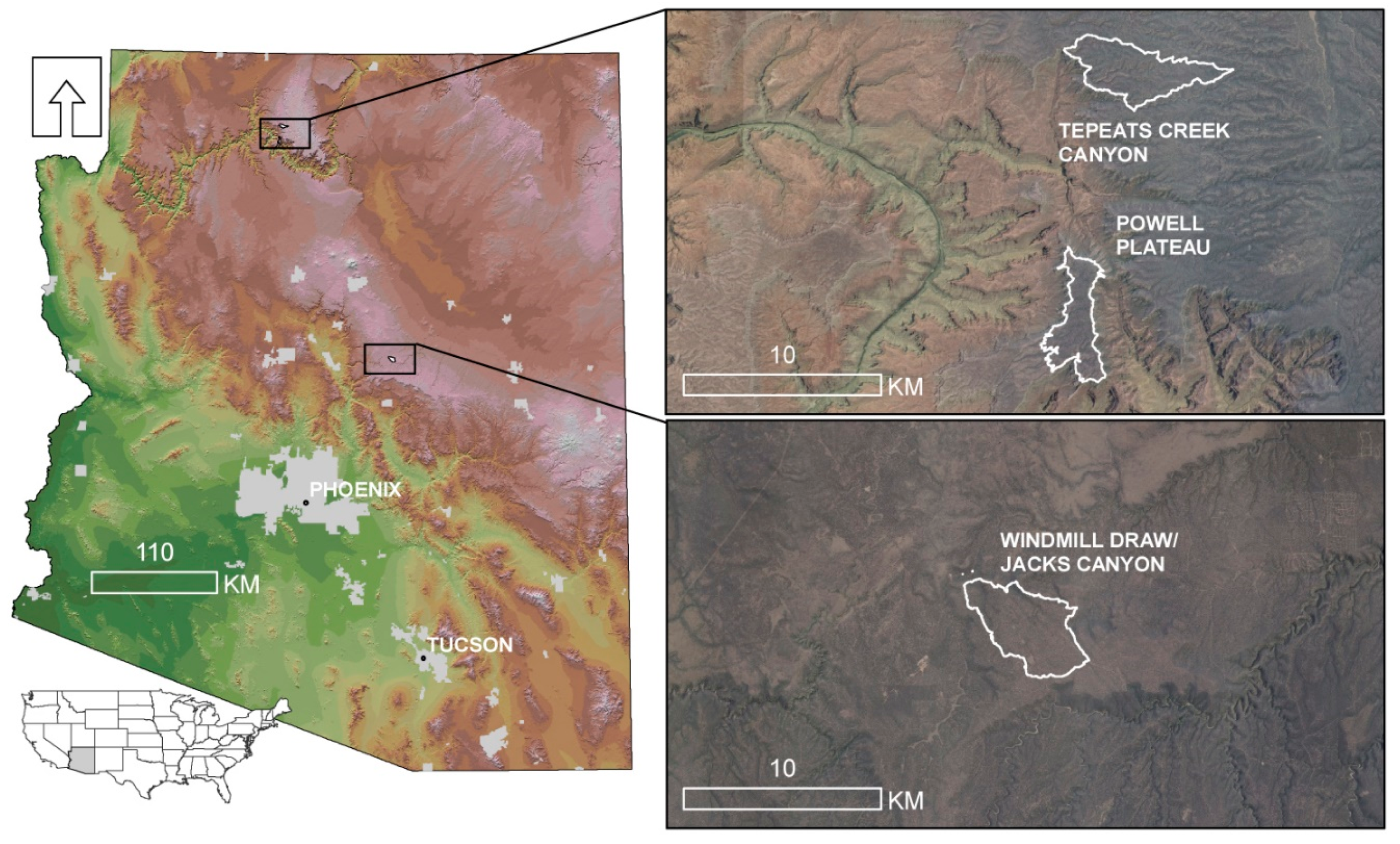
Figure 1.
Map of study landscapes in northern Arizona, USA. Powell Plateau and Tepeats Creek on the North Rim of the Grand Canyon, and Windmill Draw/Jacks Canyon on the Mogollon Rim.
Figure 1.
Map of study landscapes in northern Arizona, USA. Powell Plateau and Tepeats Creek on the North Rim of the Grand Canyon, and Windmill Draw/Jacks Canyon on the Mogollon Rim.
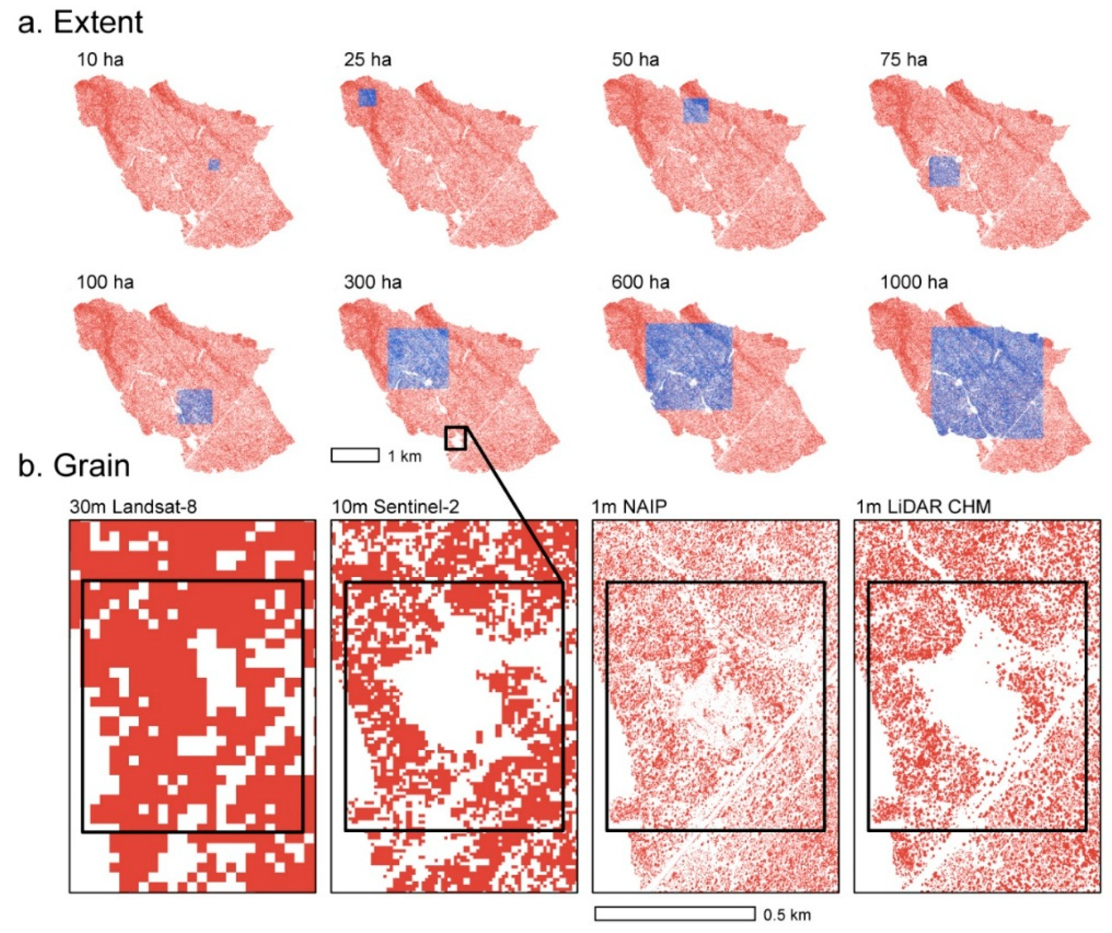
Figure 2.
Remotely sensed data products and associated grain of each data source: Landsat-8 (30 m), Sentinel-2 (10 m), NAIP (1 m), and LiDAR (1 m). The top panel (a) shows the canopy cover of Windmill Draw landscape, with the blue areas representing the relative size of each extent (10–1000 ha) analyzed. The lower panel (b) shows size of the spatial grain (resolution) and level of information available for each data product within an example extent.
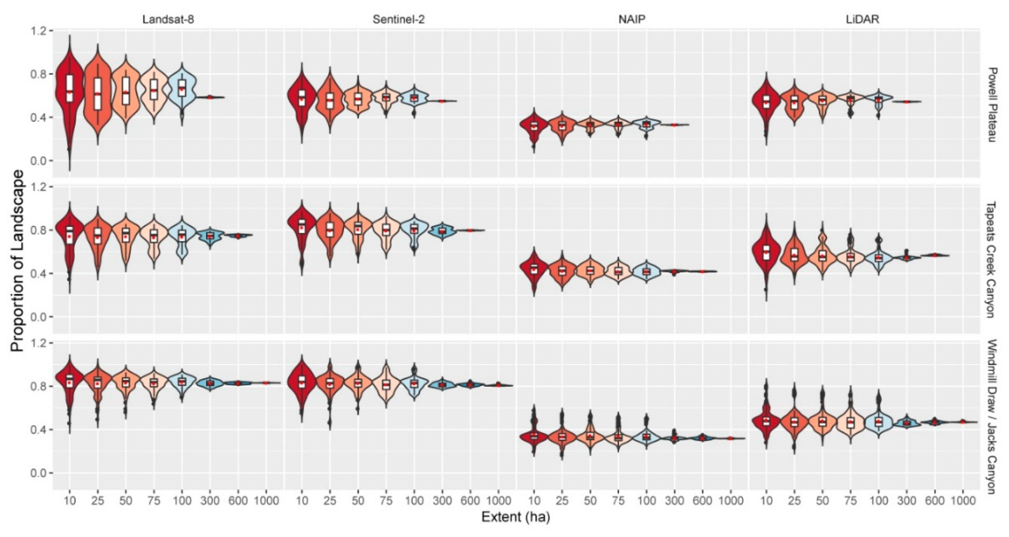
Figure 3.
Violin plots (colored by extent and depicting probability density of the data at different values smoothed by a kernel density estimator), box-and-whisker plots (black and white), and mean (red dot) for the proportion of landscape (ha) under forested canopy cover for each landscape and data product (Landsat-8 30 m, Sentinel-2 10 m, NAIP 1 m, LiDAR 1 m), and across multiple spatial extents. Insets with rescaled y-axis provided for clarity.
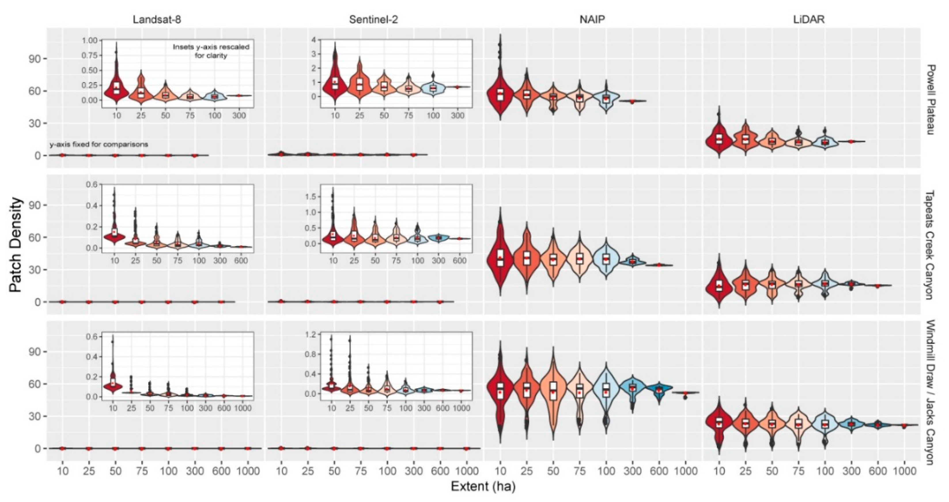
Figure 4.
Violin plots (colored by extent and depicting probability density of the data at different values smoothed by a kernel density estimator), box-and-whisker plots (black and white) and mean (red dot) for patch density (patches per ha). Patch density is the number of patches per landscape area under forested canopy cover for each landscape and data product (Landsat-8 30 m, Sentinel-2 10 m, NAIP 1 m, LiDAR 1 m), and across multiple spatial extents. Insets with rescaled y-axis provided for clarity.
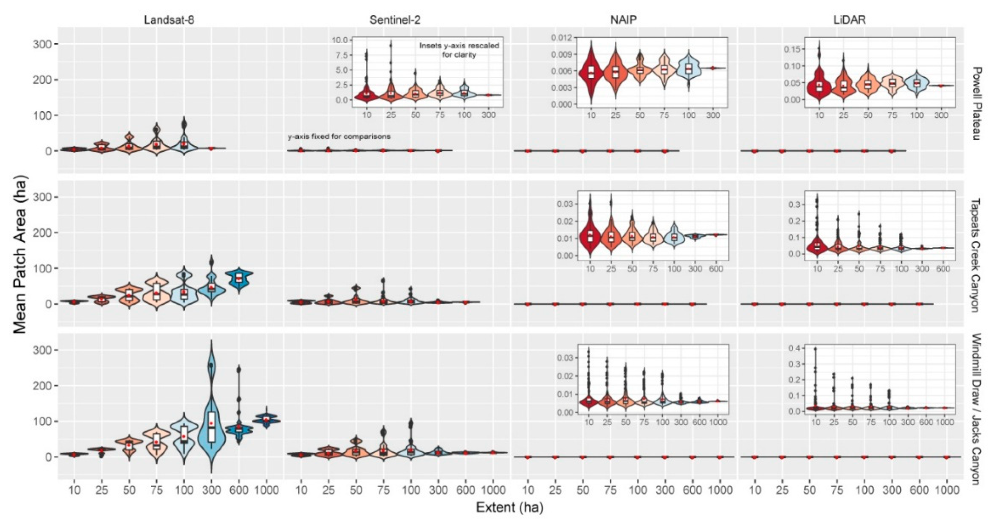
Figure 5.
Violin plots (colored by extent and depicting probability density of the data at different values smoothed by a kernel density estimator), box-and-whisker plots (black and white), and mean (red dot) for mean patch area (ha) (average size of patches) for each landscape and data product (Landsat-8 30 m, Sentinel-2 10 m, NAIP 1 m, LiDAR 1 m), and across multiple spatial extents. Insets with rescaled y-axis provided for clarity.
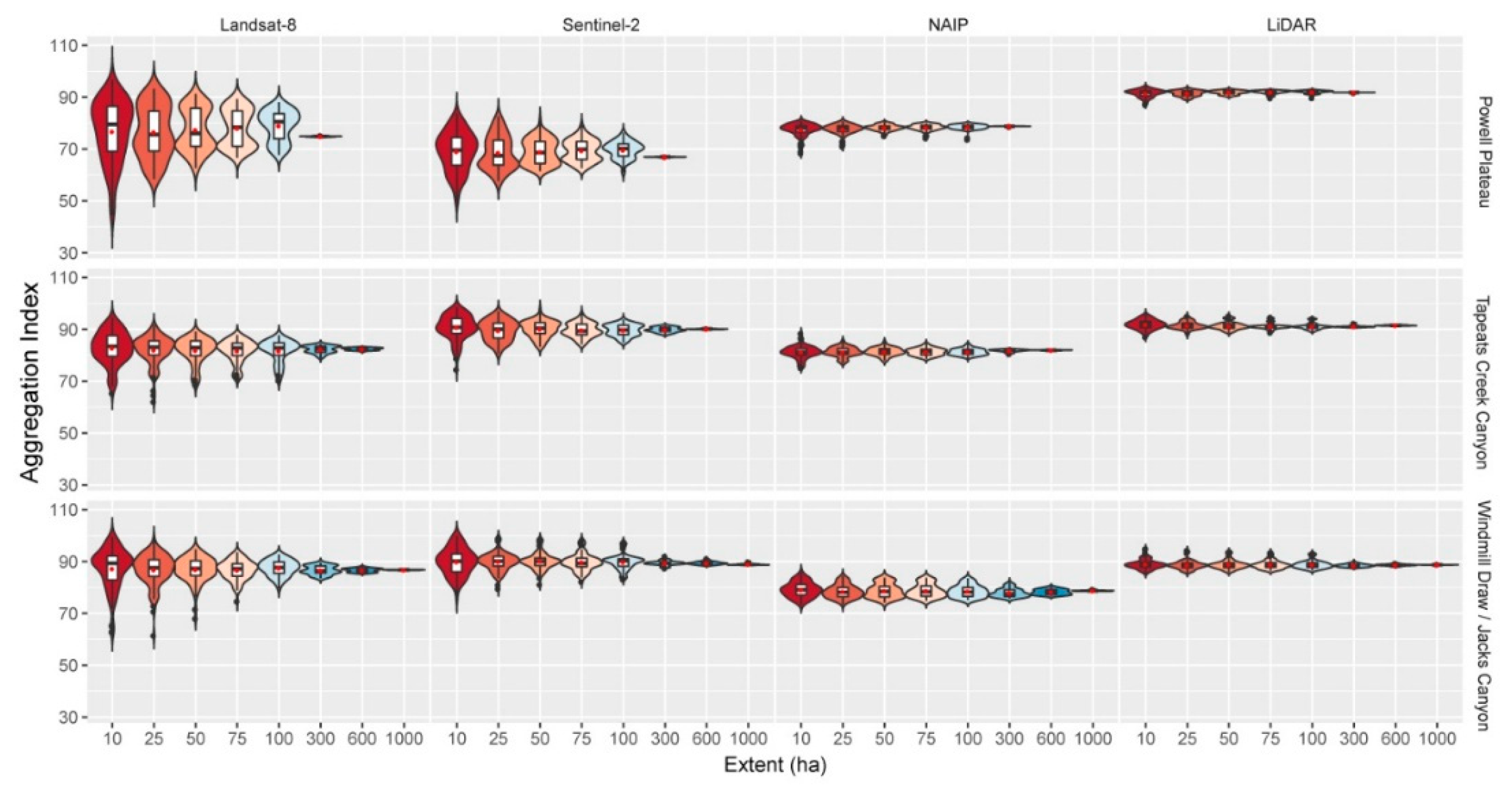
Figure 6.
Violin plots (colored by extent and depicting probability density of the data at different values smoothed by a kernel density estimator), box-and-whisker plots (black and white) and mean (red dot) for aggregation index (0–100). Aggregation index indicates how adjacent patches of canopy cover are to each other for each landscape and data product (Landsat-8 30 m, Sentinel-2 10 m, NAIP 1 m, LiDAR 1 m), and across multiple spatial extents. Insets with rescaled y-axis provided for clarity.
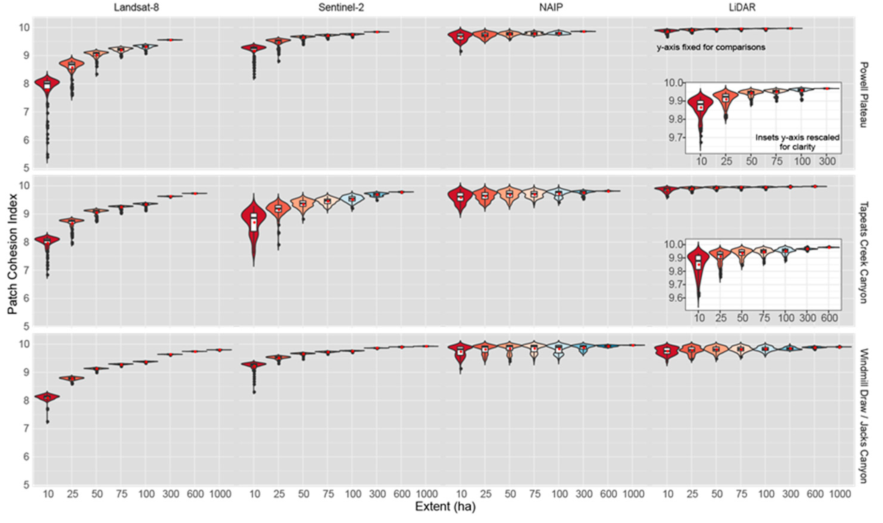
Figure 7.
Violin plots (colored by extent and depicting probability density of the data at different values smoothed by a kernel density estimator), box-and-whisker plots (black and white) and mean (red dot) for patch cohesion index (%). Patch cohesion index describes the physical connectedness of patches of canopy cover for each landscape and data product (Landsat-8 30 m, Sentinel-2 10 m, NAIP 1 m, LiDAR 1 m), and across multiple spatial extents. Insets with rescaled y-axis provided for clarity.
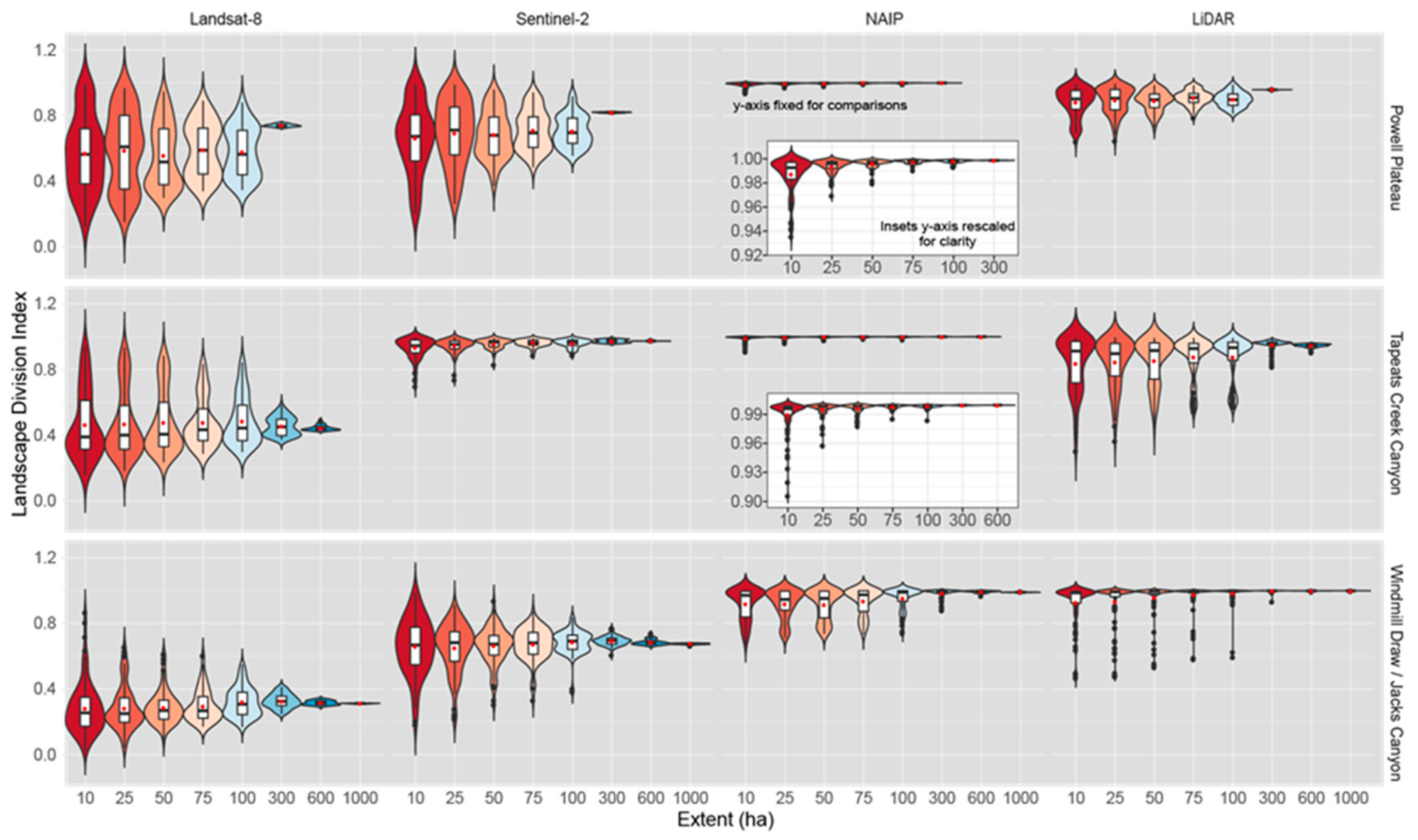
Figure 8.
Violin plots (colored by extent and depicting probability density of the data at different values smoothed by a kernel density estimator), box-and-whisker plots (black and white) and mean (red dot) for landscape division index (%). Landscape division index is presented for each landscape and data product (Landsat-8 30 m, Sentinel-2 10 m, NAIP 1 m, LiDAR 1 m), and across multiple spatial extents and is defined as the probability that two animals placed in different areas somewhere in the extent might find one another. Insets with rescaled y-axis provided for clarity.
Table 2.
Proportion of landscape (PLand) comprised of canopy cover across each landscape and data product (Landsat-8 30 m, Sentinel-2 10 m, NAIP 1 m, LiDAR 1 m), and across multiple spatial extents. Mean values and standard error (SE) are shown.
Table 2.
Proportion of landscape (PLand) comprised of canopy cover across each landscape and data product (Landsat-8 30 m, Sentinel-2 10 m, NAIP 1 m, LiDAR 1 m), and across multiple spatial extents. Mean values and standard error (SE) are shown.
| Proportion of Landscape (%) Extent (ha) | | | | | |
|---|
| | 10 | 25 | 50 | 75 | 100 | 300 | 600 | 1000 |
|---|
| Powell Plateau | | | | | | | | |
| Landsat-8 | 0.633 (0.019) | 0.619 (0.017) | 0.635 (0.013) | 0.648 (0.011) | 0.660 (0.009) | 0.584 (0.000) | | |
| Sentinel-2 | 0.568 (0.011) | 0.559 (0.010) | 0.569 (0.006) | 0.578 (0.005) | 0.577 (0.004) | 0.550 (0.000) | | |
| NAIP | 0.314 (0.006) | 0.319 (0.005) | 0.330 (0.003) | 0.332 (0.003) | 0.334 (0.003) | 0.329 (0.000) | | |
| LiDAR | 0.537 (0.010) | 0.535 (0.007) | 0.552 (0.006) | 0.560 (0.005) | 0.560 (0.004) | 0.543 (0.000) | | |
| Tepeats Creek | | | | | | | | |
| Landsat-8 | 0.743 (0.013) | 0.734 (0.011) | 0.742 (0.009) | 0.732 (0.009) | 0.737 (0.008) | 0.744 (0.003) | 0.748 (0.001) | |
| Sentinel-2 | 0.824 (0.011) | 0.797 (0.009) | 0.807 (0.008) | 0.795 (0.008) | 0.796 (0.007) | 0.790 (0.003) | 0.797 (0.000) | |
| NAIP | 0.439 (0.007) | 0.422 (0.006) | 0.427 (0.005) | 0.418 (0.004) | 0.417 (0.004) | 0.420 (0.001) | 0.418 (0.000) | |
| LiDAR | 0.596 (0.010) | 0.571 (0.008) | 0.565 (0.008) | 0.560 (0.007) | 0.550 (0.007) | 0.546 (0.002) | 0.568 (0.001) | |
| Windmill Draw | | | | | | | | |
| Landsat-8 | 0.835 (0.010) | 0.826 (0.009) | 0.832 (0.007) | 0.824 (0.006) | 0.838 (0.005) | 0.826 (0.002) | 0.828 (0.001) | 0.831 (0.000) |
| Sentinel-2 | 0.832 (0.009) | 0.819 (0.009) | 0.828 (0.007) | 0.816 (0.007) | 0.824 (0.006) | 0.813 (0.002) | 0.814 (0.001) | 0.809 (0.001) |
| NAIP | 0.356 (0.008) | 0.336 (0.007) | 0.347 (0.006) | 0.339 (0.006) | 0.341 (0.005) | 0.321 (0.002) | 0.321 (0.001) | 0.318 (0.000) |
| LiDAR | 0.492 (0.010) | 0.473 (0.009) | 0.484 (0.008) | 0.476 (0.008) | 0.480 (0.007) | 0.461 (0.002) | 0.467 (0.001) | 0.470 (0.000) |
Table 3.
Patch density (PD), the average number of patches of canopy cover on each landscape, delineated by each data product (Landsat-8 30 m, Sentinel-2 10 m, NAIP 1 m, LiDAR 1 m) and across multiple spatial extents. Mean values and standard error (SE) are shown.
Table 3.
Patch density (PD), the average number of patches of canopy cover on each landscape, delineated by each data product (Landsat-8 30 m, Sentinel-2 10 m, NAIP 1 m, LiDAR 1 m) and across multiple spatial extents. Mean values and standard error (SE) are shown.
| Patch Density (ha) | Extent (ha) | | | | | | |
|---|
| | 10 | 25 | 50 | 75 | 100 | 300 | 600 | 1000 |
|---|
| Powell Plateau | | | | | | | | |
| Landsat-8 | 0.214 (0.015) | 0.138 (0.011) | 0.090 (0.006) | 0.063 (0.004) | 0.061 (0.004) | 0.075 (0.000) | | |
| Sentinel-2 | 1.047 (0.074) | 0.883 (0.053) | 0.706 (0.035) | 0.597 (0.028) | 0.590 (0.025) | 0.673 (0.002) | | |
| NAIP | 57.969 (1.079) | 56.659 (0.695) | 53.808 (0.516) | 53.300 (0.499) | 52.735 (0.448) | 50.537 (0.025) | | |
| LiDAR | 15.428 (0.661) | 15.170 (0.536) | 13.349 (0.377) | 12.601 (0.352) | 12.375 (0.302) | 12.950 (0.011) | | |
| Tepeats Creek | | | | | | | | |
| Landsat-8 | 0.153 (0.010) | 0.085 (0.007) | 0.051 (0.004) | 0.041 (0.003) | 0.038 (0.003) | 0.019 (0.001) | 0.011 (0.000) | |
| Sentinel-2 | 0.310 (0.032) | 0.259 (0.023) | 0.189 (0.017) | 0.207 (0.015) | 0.185 (0.014) | 0.182 (0.005) | 0.157 (0.000) | |
| NAIP | 41.339 (1.283) | 40.980 (1.027) | 39.345 (0.835) | 40.110 (0.723) | 39.728 (0.626) | 37.624 (0.212) | 34.257 (0.041) | |
| LiDAR | 15.310 (0.750) | 16.167 (0.617) | 16.325 (0.616) | 16.551 (0.526) | 16.973 (0.487) | 16.740 (0.135) | 15.306 (0.022) | |
| Windmill Draw | | | | | | | | |
| Landsat-8 | 0.138 (0.007) | 0.056 (0.004) | 0.032 (0.002) | 0.030 (0.003) | 0.021 (0.002) | 0.013 (0.001) | 0.011 (0.000) | 0.008 (0.000) |
| Sentinel-2 | 0.205 (0.018) | 0.153 (0.018) | 0.099 (0.009) | 0.104 (0.008) | 0.081 (0.006) | 0.073 (0.002) | 0.072 (0.001) | 0.067 (0.000) |
| NAIP | 52.483 (1.502) | 54.286 (1.227) | 52.324 (1.362) | 52.001 (1.231) | 52.385 (1.146) | 55.683 (0.579) | 54.084 (0.352) | 51.462 (0.104) |
| LiDAR | 23.018 (0.853) | 23.109 (0.691) | 22.289 (0.706) | 21.886 (0.663) | 21.978 (0.618) | 22.724 (0.238) | 21.838 (0.135) | 21.666 (0.040) |
Table 4.
Mean Patch Area (MPA) (ha), the average area composed of patches of canopy cover, across each landscape and data product (Landsat-8 30 m, Sentinel-2 10 m, NAIP 1 m, LiDAR 1 m), and across multiple spatial extents. Mean values and standard error (SE) are shown.
Table 4.
Mean Patch Area (MPA) (ha), the average area composed of patches of canopy cover, across each landscape and data product (Landsat-8 30 m, Sentinel-2 10 m, NAIP 1 m, LiDAR 1 m), and across multiple spatial extents. Mean values and standard error (SE) are shown.
| Mean Patch Area (ha) | Extent (ha) | | | | | | |
|---|
| | 10 | 25 | 50 | 75 | 100 | 300 | 600 | 1000 |
|---|
| Powell Plateau | | | | | | | | |
| Landsat-8 | 4.647 (0.299) | 9.474 (0.776) | 13.988 (1.296) | 19.518 (1.840) | 20.520 (2.052) | 7.819 (0.035) | | |
| Sentinel-2 | 1.094 (0.132) | 1.158 (0.129) | 1.096 (0.069) | 1.245 (0.067) | 1.206 (0.061) | 0.817 (0.002) | | |
| NAIP | 0.006 (0.000) | 0.006 (0.000) | 0.006 (0.000) | 0.006 (0.000) | 0.006 (0.000) | 0.007 (0.000) | | |
| LiDAR | 0.045 (0.003) | 0.042 (0.002) | 0.046 (0.002) | 0.048 (0.001) | 0.048 (0.001) | 0.042 (0.000) | | |
| Tepeats Creek | | | | | | | | |
| Landsat-8 | 6.351 (0.264) | 13.949 (0.736) | 25.349 (1.542) | 31.540 (2.152) | 34.500 (2.566) | 47.600 (2.326) | 71.374 (1.401) | |
| Sentinel-2 | 5.420 (0.344) | 7.333 (0.700) | 12.646 (1.459) | 8.224 (1.062) | 7.709 (0.663) | 4.834 (0.187) | 5.082 (0.014) | |
| NAIP | 0.012 (0.001) | 0.011 (0.000) | 0.012 (0.000) | 0.011 (0.000) | 0.011 (0.000) | 0.011 (0.000) | 0.012(0.000) |
| LiDAR | 0.059 (0.006) | 0.045 (0.003) | 0.046 (0.004) | 0.041 (0.003) | 0.038 (0.002) | 0.033 (0.000) | 0.037 (0.000) | |
| Windmill Draw | | | | | | | | |
| Landsat-8 | 7.248 (0.255) | 18.257 (0.611) | 33.437 (1.340) | 42.230 (2.231) | 58.305 (2.789) | 95.256 (6.883) | 85.781 (3.900) | 104.836 (0.889) |
| Sentinel-2 | 6.083 (0.302) | 11.371 (0.782) | 17.674 (1.437) | 19.018 (2.053) | 20.103 (2.224) | 12.738 (0.508) | 11.511 (0.152) | 12.085 (0.100) |
| NAIP | 0.008 (0.001) | 0.007 (0.000) | 0.008 (0.000) | 0.008 (0.000) | 0.007 (0.000) | 0.006 (0.000) | 0.006 (0.000) | 0.006 (0.000) |
| LiDAR | 0.035 (0.005) | 0.028 (0.004) | 0.030 (0.004) | 0.029 (0.003) | 0.028 (0.002) | 0.021 (0.000) | 0.022 (0.000) | 0.022 (0.000) |
Table 5.
Aggregation index (AI) (%) of canopy cover across each landscape and data product (Landsat-8 30 m, Sentinel-2 10 m, NAIP 1 m, LiDAR 1 m), and across multiple spatial extents. Mean values and standard error (SE) are shown.
Table 5.
Aggregation index (AI) (%) of canopy cover across each landscape and data product (Landsat-8 30 m, Sentinel-2 10 m, NAIP 1 m, LiDAR 1 m), and across multiple spatial extents. Mean values and standard error (SE) are shown.
| Aggregation Index | Extent (ha) | | | | | | |
|---|
| | 10 | 25 | 50 | 75 | 100 | 300 | 600 | 1000 |
|---|
| Powell Plateau | | | | | | | | |
| Landsat-8 | 76.761 (1.175) | 76.553 (0.986) | 77.397 (0.802) | 78.012 (0.712) | 78.950 (0.581) | 74.823 (0.021) | | |
| Sentinel-2 | 69.008 (0.748) | 68.585 (0.636) | 68.873 (0.473) | 69.394 (0.406) | 69.600 (0.323) | 66.906 (0.009) | | |
| NAIP | 77.402 (0.246) | 77.603 (0.191) | 78.206 (0.113) | 78.239 (0.122) | 78.429 (0.105) | 78.773 (0.003) | | |
| LiDAR | 91.447 (0.146) | 91.467 (0.106) | 91.810 (0.074) | 91.921 (0.070) | 91.941 (0.063) | 91.810 (0.001) | | |
| Tepeats Creek | | | | | | | | |
| Landsat-8 | 82.820 (0.625) | 82.027 (0.543) | 81.855 (0.490) | 81.684 (0.425) | 81.706 (0.426) | 82.238 (0.139) | 82.418 (0.047) | |
| Sentinel-2 | 90.755 (0.471) | 89.497 (0.390) | 90.100 (0.311) | 89.688 (0.269) | 89.613 (0.221) | 89.824 (0.094) | 90.086 (0.012) | |
| NAIP | 81.195 (0.239) | 81.281 (0.183) | 81.362 (0.150) | 81.272 (0.137) | 81.256 (0.121) | 81.784 (0.047) | 81.914 (0.013) | |
| LiDAR | 91.847 (0.181) | 91.468 (0.144) | 91.330 (0.146) | 91.286 (0.127) | 91.147 (0.118) | 91.083 (0.041) | 91.506 (0.013) | |
| Windmill Draw | | | | | | | | |
| Landsat-8 | 87.235 (0.775) | 86.813 (0.595) | 86.940 (0.466) | 86.730 (0.364) | 87.511 (0.305) | 86.643 (0.168) | 86.639 (0.073) | 86.754 (0.010) |
| Sentinel-2 | 89.880 (0.514) | 89.913 (0.344) | 90.184 (0.312) | 89.781 (0.323) | 89.827 (0.298) | 89.461 (0.091) | 89.408 (0.061) | 88.922 (0.032) |
| NAIP | 79.129 (0.287) | 78.427 (0.252) | 78.715 (0.271) | 78.745 (0.256) | 78.549 (0.231) | 77.921 (0.159) | 78.242 (0.102) | 78.734 (0.020) |
| LiDAR | 88.984 (0.192) | 88.656 (0.170) | 88.852 (0.175) | 88.824 (0.163) | 88.834 (0.151) | 88.463 (0.057) | 88.651 (0.035) | 88.751 (0.008) |
Table 6.
Patch cohesion (PC) index measuring the physical connectedness of patches of canopy cover for each landscape and data product (Landsat-8 30 m, Sentinel-2 10 m, NAIP 1 m, LiDAR 1 m), and across spatial extents. Mean values and standard error (SE) are shown.
Table 6.
Patch cohesion (PC) index measuring the physical connectedness of patches of canopy cover for each landscape and data product (Landsat-8 30 m, Sentinel-2 10 m, NAIP 1 m, LiDAR 1 m), and across spatial extents. Mean values and standard error (SE) are shown.
| Patch Cohesion Index (%) | | Extent (ha) | | | | |
|---|
| | 10 | 25 | 50 | 75 | 100 | 300 | 600 | 1000 |
|---|
| Powell Plateau | | | | | | | | |
| Landsat-8 | 7.733 (0.066) | 8.496 (0.036) | 8.998 (0.014) | 9.205 (0.008) | 9.318 (0.005) | 9.560 (0.000) | | |
| Sentinel-2 | 9.183 (0.020) | 9.476 (0.012) | 9.654 (0.004) | 9.723 (0.002) | 9.760 (0.001) | 9.855 (0.000) | | |
| NAIP | 9.539 (0.015) | 9.624 (0.013) | 9.686 (0.008) | 9.686 (0.006) | 9.705 (0.004) | 9.733 (0.000) | | |
| LiDAR | 9.859 (0.007) | 9.914 (0.003) | 9.947 (0.001) | 9.957 (0.001) | 9.963 (0.001) | 9.979 (0.000) | | |
| Tepeats Creek | | | | | | | | |
| Landsat-8 | 7.970 (0.024) | 8.700 (0.012) | 9.063 (0.010) | 9.229 (0.009) | 9.331 (0.007) | 9.627 (0.001) | 9.731 (0.000) | |
| Sentinel-2 | 9.327 (0.008) | 9.569 (0.004) | 9.697 (0.002) | 9.749 (0.002) | 9.785 (0.001) | 9.877 (0.000) | 9.911 (0.000) | |
| NAIP | 9.758 (0.013) | 9.793 (0.011) | 9.835 (0.009) | 9.844 (0.008) | 9.850 (0.008) | 9.913 (0.003) | 9.947 (0.000) | |
| LiDAR | 9.887 (0.006) | 9.919 (0.004) | 9.936 (0.003) | 9.947 (0.002) | 9.949 (0.002) | 9.971 (0.000) | 9.981 (0.000) | |
| Windmill Draw | | | | | | | | |
| Landsat-8 | 8.070 (0.015) | 8.767 (0.006) | 9.126 (0.003) | 9.283 (0.002) | 9.378 (0.001) | 9.638 (0.000) | 9.743 (0.000) | 9.798 (0.000) |
| Sentinel-2 | 9.333 (0.005) | 9.571 (0.005) | 9.698 (0.002) | 9.752 (0.002) | 9.784 (0.002) | 9.876 (0.000) | 9.912 (0.000) | 9.932 (0.000) |
| NAIP | 9.476 (0.021) | 9.471 (0.019) | 9.551 (0.020) | 9.538 (0.020) | 9.561 (0.019) | 9.518 (0.012) | 9.554 (0.009) | 9.627 (0.002) |
| LiDAR | 9.759 (0.012) | 9.793 (0.010) | 9.839 (0.008) | 9.843 (0.009) | 9.858 (0.008) | 9.876 (0.004) | 9.906 (0.002) | 9.921 (0.000) |
Table 7.
Landscape division index (LDI) of canopy cover across all three landscapes across for each data product (Landsat-8 30 m, Sentinel-2 10 m, NAIP 1 m, LiDAR 1 m), and across multiple spatial extents. Mean values and standard error (SE) are shown.
Table 7.
Landscape division index (LDI) of canopy cover across all three landscapes across for each data product (Landsat-8 30 m, Sentinel-2 10 m, NAIP 1 m, LiDAR 1 m), and across multiple spatial extents. Mean values and standard error (SE) are shown.
| Landscape Division Index | | Extent | | | | | |
|---|
| | 10 | 25 | 50 | 75 | 100 | 300 | 600 | 1000 |
|---|
| Powell Plateau | | | | | | | | |
| Landsat-8 | 0.585 (0.024) | 0.628 (0.025) | 0.615 (0.020) | 0.594 (0.016) | 0.581 (0.014) | 0.741 (0.001) | | |
| Sentinel-2 | 0.708 (0.015) | 0.726 (0.014) | 0.708 (0.010) | 0.692 (0.008) | 0.695 (0.006) | 0.745 (0.000) | | |
| NAIP | 0.996 (0.000) | 0.997 (0.000) | 0.998 (0.000) | 0.999 (0.000) | 0.999 (0.000) | 1.000 (0.000) | | |
| LiDAR | 0.869 (0.012) | 0.879 (0.010) | 0.867 (0.007) | 0.864 (0.006) | 0.859 (0.006) | 0.881 (0.000) | | |
| Tepeats Creek | | | | | | | | |
| Landsat-8 | 0.446 (0.021) | 0.468 (0.018) | 0.474 (0.018) | 0.489 (0.017) | 0.486 (0.016) | 0.453 (0.006) | 0.444 (0.001) | |
| Sentinel-2 | 0.326 (0.020) | 0.382 (0.017) | 0.367 (0.016) | 0.394 (0.016) | 0.382 (0.013) | 0.385 (0.005) | 0.374 (0.000) | |
| NAIP | 0.959 (0.005) | 0.977 (0.003) | 0.980 (0.003) | 0.986 (0.002) | 0.988 (0.002) | 0.994 (0.000) | 0.994 (0.000) | |
| LiDAR | 0.775 (0.017) | 0.839 (0.013) | 0.852 (0.015) | 0.869 (0.013) | 0.893 (0.012) | 0.939 (0.004) | 0.936 (0.001) | |
| Windmill Draw | | | | | | | | |
| Landsat-8 | 0.305 (0.018) | 0.319 (0.015) | 0.310 (0.012) | 0.325 (0.010) | 0.301 (0.008) | 0.322 (0.004) | 0.318 (0.001) | 0.312 (0.000) |
| Sentinel-2 | 0.319 (0.018) | 0.344 (0.017) | 0.337 (0.015) | 0.358 (0.016) | 0.353 (0.015) | 0.366 (0.006) | 0.366 (0.005) | 0.354 (0.001) |
| NAIP | 0.983 (0.005) | 0.992 (0.003) | 0.990 (0.003) | 0.994 (0.002) | 0.995 (0.002) | 1.000 (0.000) | 1.000 (0.000) | 1.000 (0.000) |
| LiDAR | 0.925 (0.014) | 0.957 (0.011) | 0.952 (0.011) | 0.964 (0.009) | 0.965 (0.009) | 0.997 (0.000) | 0.998 (0.000) | 0.998 (0.000) |


