Geographically Weighted Negative Binomial Regression Model Predicts Wildfire Occurrence in the Great Xing’an Mountains Better Than Negative Binomial Model

Abstract

Wildfire is a major disturbance that affects large area globally every year. Thus, a better prediction of the likelihood of wildfire occurrence is essential to develop appropriate fire prevention measures. We applied a global negative Binomial (NB) and a geographically weighted negative Binomial regression (GWNBR) models to determine the relationship between wildfire occurrence and its drivers factors in the boreal forests of the Great Xing’an Mountains, northeast China. Using geo-weighted techniques to consider the geospatial information of meteorological, topographic, vegetation type and human factors, we aimed to verify whether the performance of the NB model can be improved. Our results confirmed that the model fitting and predictions of GWNBR model were better than the global NB model, produced more precise and stable model parameter estimation, yielded a more realistic spatial distribution of model predictions, and provided the detection of the impact hotpots of these predictor variables. We found slope, vegetation cover, average precipitation, average temperature, and average relative humidity as important predictors of wildfire occurrence in the Great Xing’an Mountains. Thus, spatially differing relations improves the explanatory power of the global NB model, which does not explain sufficiently the relationship between wildfire occurrence and its drivers. Thus, the GWNBR model can complement the global NB model in overcoming the issue of nonstationary variables, thereby enabling a better prediction of the occurrence of wildfires in large geographical areas and improving management practices of wildfire.

1. Introduction

Fires are an important ecological factor that affect the renewal and succession of forest vegetation and cause damage to forest ecosystems [1]. In China, for instance, about 10,000 wildfires occur with approximately 820,000 hectares burnt area each year [2]. The Chinese boreal forest, especially the Great Xing’an Mountains set in northeastern of China, has a wide range of forest resource, and is vulnerable to frequent wildfires [3,4]. Thus, understanding the characteristics of wildfire occurrence in the region and establishing a wildfire occurrence prediction model has become the key to local wildfire management.

Exploring wildfire drivers is essential to develop wildfire prediction models. Many studies found that environmental factors such as meteorology, vegetation, and topography play a key role in the occurrence and spread of wildfires [5,6,7,8,9,10,11]. Changes in meteorological factors, such as temperature, relative humidity, and precipitation, influence the moisture content of the fuel, which in turn affects the ignition and spread of wildfires [9,12,13]. Topographic variation affects the composition of vegetation and the spatial distribution of fuel, forming different fire environments, thus directly affecting the occurrence and the spread of wildfires [14]. Furthermore, human activities and socio-economic conditions, such as population density and human settlements, have a significant effect on wildfire occurrence [6].

To predict the number of wildfire occurrence, Poisson regression models have been frequently employed [15,16,17]. Its assumption is equality between the sample mean and variance. In practice, however, wildfire data (e.g., the number of wildfires occurrence) are often excessively discrete with unequal mean and variance, resulting in large errors in Poisson regression estimation results. When the sample variance exceeds the sample mean; i.e., over-dispersion, negative binomial (NB) models is an alternative modeling approach for count data [18]. The problem with the classical regression model is its assumption, which is the spatial stationary of the relationship between the response variable and the explanatory variable [19]. Many researchers have found that the model parameters are not stationary (i.e., constant) over large study areas, but have spatial differences [20,21,22]. It has been shown that drivers of wildfire and wildfire source conditions are spatially explicit in different forest ecosystems [4,23,24]. Thus, the assumption of spatial stability of the global model may obscure the true relationship between the explanatory and the response variables.

Thus, it is imperative to consider spatial relationships between wildfire and their underlying drivers to develop an effective and realistic prediction models. Geographically weighted regression (GWR) can effectively resolve the spatial non-stationarity problem [25]. This method takes into account the effects of geospatial factors and is able to incorporate spatial variations of explanatory variables into the model. GWR was applied in the field of wildfire research, which provides a local linear model with a reasonable explanation for the spatial variation of wildfire occurrence and its driving factors [4,22,26]. In this study, the Negative Binomial Regression (NB) and Geographically Weighted Negative Binomial Regression (GWNBR) were applied to develop wildfire prediction model with the following objectives: (1) exploring whether the relationship between wildfire and its drivers is global or spatial; (2) identifying the potential drivers of wildfire occurrence from meteorological, topographic, vegetation and human factors; and (3) further exploring spatial variability by identifying significant factors, which can eventually explain spatial variability parameters. Our hypothesis was that geospatial information of wildfire drivers would increase the explanatory power of the wildfire prediction model.

2. Materials and Methods

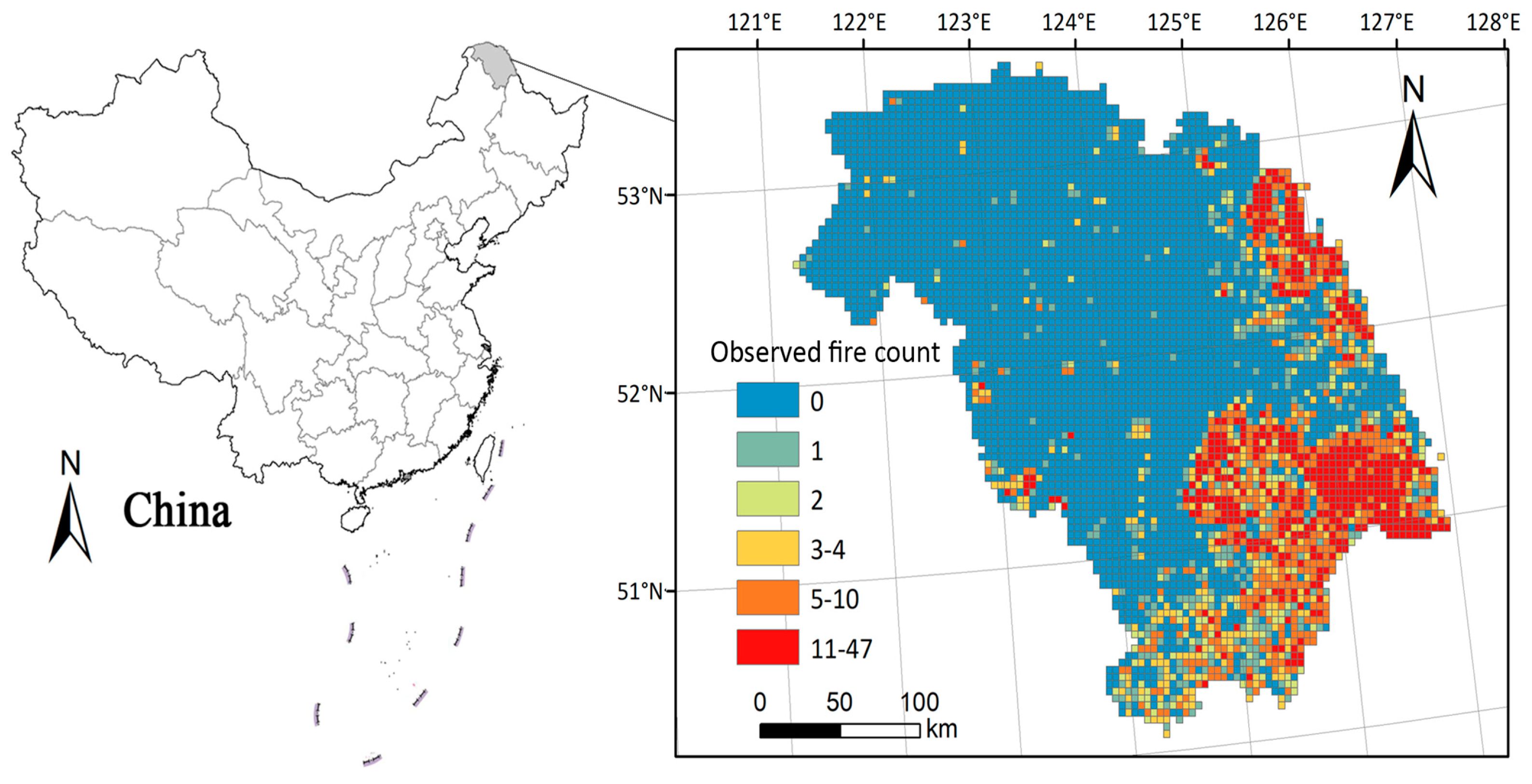
2.1. Study Area

The study was conducted in the Great Xing’an Mountain of Northeast China (50°10′–53°33′ N and 121°12′–127°00′ E), which is the southernmost part of the global forest biome (Figure 1). Its total area covers 8.46 × 106 ha, with an average elevation of 573 m. The area lies in a cold-temperate zone with an average annual temperature of −6 to 1 °C, an average annual precipitation of 240–442 mm, and rainfall concentrated in June–August. The dominant species is Dahurian larch (Larix gmelini Rupr.), Mongolian pine (Pinus sylvestris L. var. mongolica Litv.), accompanied by white birch (Betula platyphylla Suk.), aspen (Populus davidiana Dode.), and sweet poplar (Populus suaveolens Fisch.), while hade pine (Pinus pumila Reg.) is distributed in high altitude. Coniferous forests (mainly larch) have a wide distribution in the Great Xing’an Mountains and are late-stage tree species, while broadleaf forests (such as birch and poplar) are early successors due to wildfire disturbance and harvesting. The broadleaf forests are mainly found in the southern and southeastern parts of the Great Xing’an Mountains where fire spots are concentrated [3]. In addition, the fire season time in the study area consists of two periods: the spring fire season from 15 March to 15 July each year; and the fall fire season, which runs from 15 September to 15 November each year [6,14].

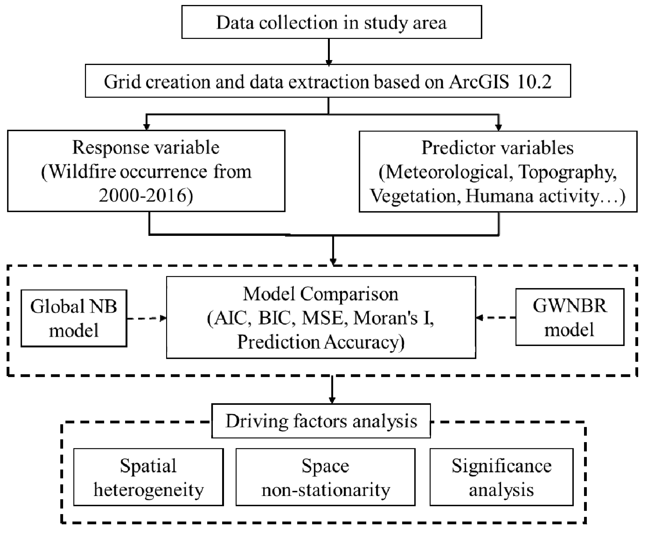
2.2. The Logical Framework of the Study

The logical framework of this study is shown in Figure 2. The response variable, which was fire points from 2000–2016, was extracted using ArcGIS in grid format together with predictor variables. Once the required data were extracted, the global NB and GWNBR models were developed and evaluated using Akaike Information Criterion (AIC), Bayesian Information Criterion (BIC), Mean Square Errors (MSE) and the Moran’s Index. The model evaluation criteria enabled identifying the spatial heterogeneity of the predictor variables. Detailed descriptions of the data extraction procedures for the response and predictor variables are given below.

2.3. Data Collection

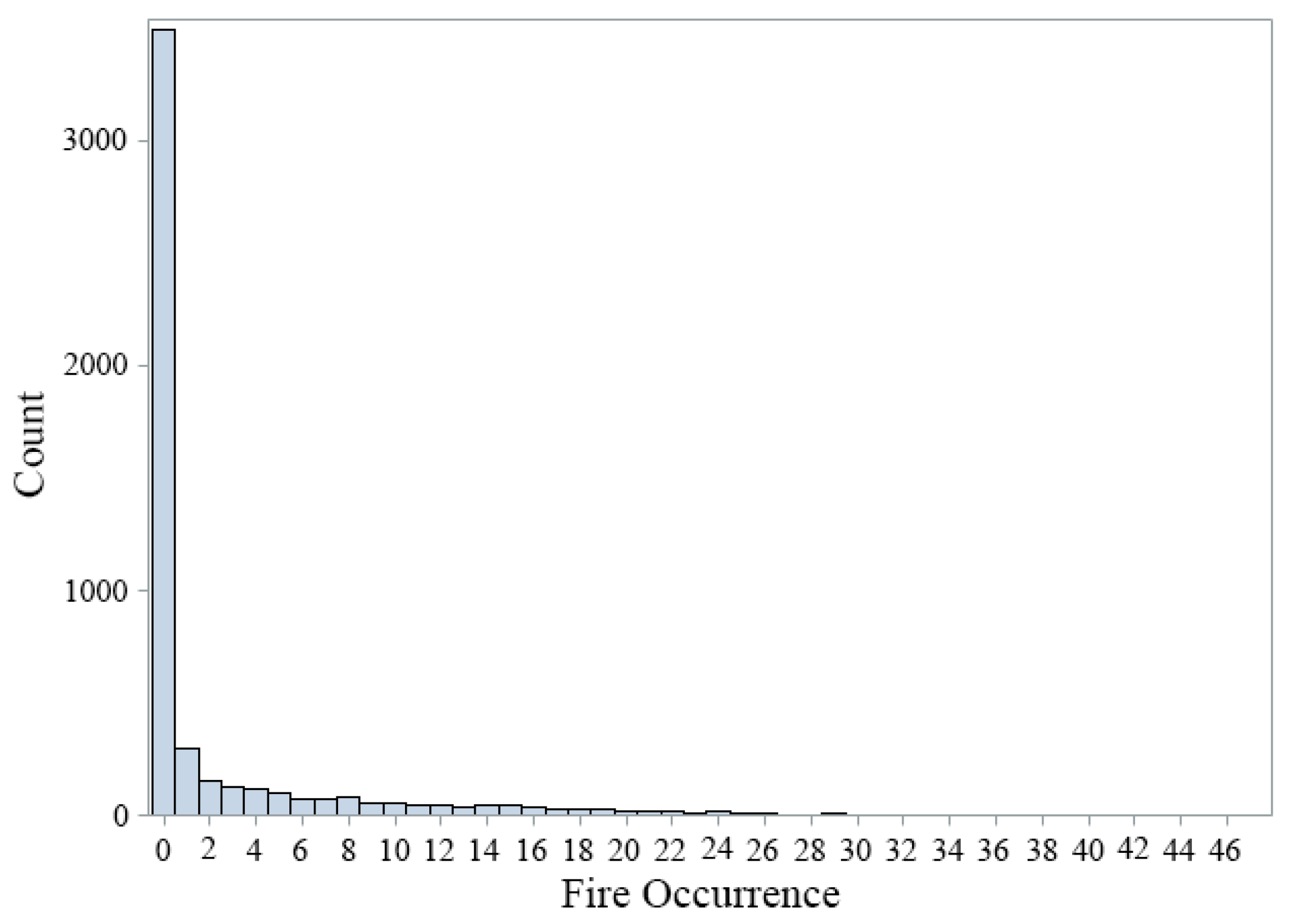
2.3.1. Response Variable

Fire frequency was the response variable, which was extracted from the Moderate Resolution Imaging Spectroradiometer (MODIS) that recorded the spatial distribution of fire pixels from 2000 to 2016. We used a daily active fire product (MOD14A1) with 1 km resolution, which is extensively applied in most recent studies [27]. However, this product cannot distinguish the type of fire, such as some non-wildfires that fall within the town, agricultural land and other areas. Therefore, the product was further processed using land use map of 1 km resolution, removing fire points falling in cities and construction sites and farmland. Fire point from 2000 to 2016 (from 15 March to 15 July and 15 September to 15 November, i.e., fire season) and its information (including geographical coordinates and time of fire occurrence) were extracted. We used ArcGIS 10.2 (released by Esri in USA in July 2013) to divide the study areas into 4 × 4 km grids (5110 grids) and calculate the total number of fire points in each grid for 16 years, respectively [28]. Figure 1 illustrates the spatial distribution of the wildfire points and Figure 3 shows the frequency distribution of the wildfire occurrence.

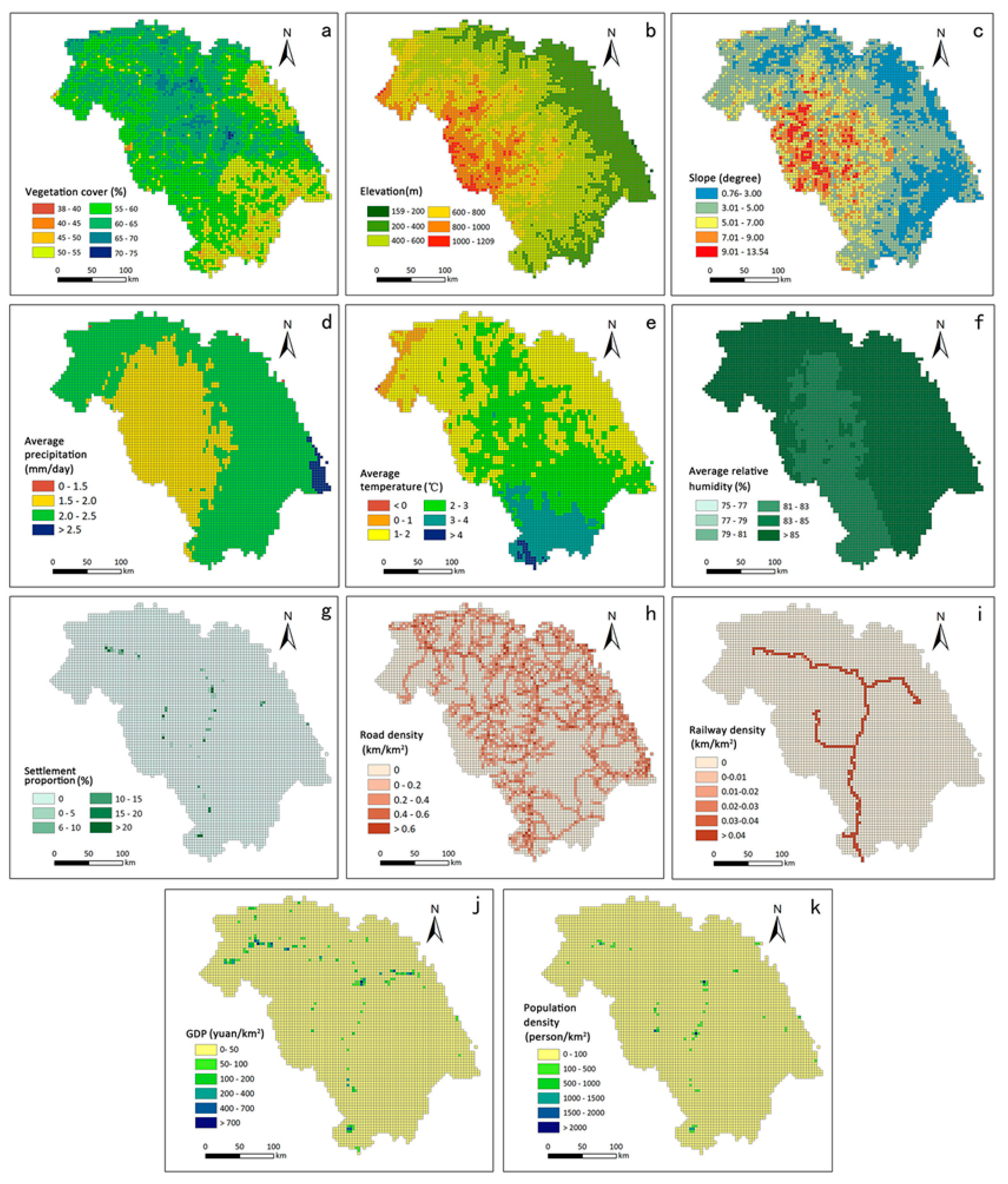
2.3.2. Predictor Variables

The predictor variables included meteorological, topographic, vegetation, and human factors, with a total 11 variables. The predictor variables were average relative humidity (%), average temperature (°C), average precipitation (mm/day), elevation (km), slope (degree), vegetation cover (%), railway density (km/km²), road density (km/km²), settlements proportion (%), GDP (Gross Domestic Product) (yuan/km²), and population density (person/km²).

Table 1. Descriptive statistics of response and predictor variables.

Variables	Mean	Median	Minimum Value	Maximum Value	Standard Deviation
Fire Occurrence (point)	2.54	0	0	47	5.6
Elevation (m)	551.8	519.9	159.4	1209.1	193.2
Slope (degree)	4.6	4.2	0.76	13.5	1.9
Railway Density (km/km2)	0.01	0	0	0.49	0.05
Road Density (km/km2)	0.12	0	0	0.89	0.16
Settlement Proportion (%)	0.001	0	0	0.558	0.016
Average Rel. Humidity (%)	85.9	85.7	74.9	89.2	1.2
Average Temperature (°C)	2.1	2.0	−0.1	4.3	0.7
Average Precipitation (mm/day)	2.1	2.1	−4.6	2.6	0.2
Vegetation Cover (%)	0.6	0.6	0.4	0.7	0.04
GDP (Gross Domestic Product) (yuan/km2)	6.9	1.9	0.03	853.7	34.2
Population Density (person/km2)	6.1	0	0	2688.4	69.1

lists the descriptive statistics of the response and predictor variables and Figure 4 shows the spatial distributions of the predictor variables across the Great Xing’an Mountains.

Weather data were derived from the HadCM2 (Hadley Climate Model) climate model, which was downloaded from the Data Sharing Infrastructure of Earth System Science (http://geodata.nju.edu.cn/Portal/index.jsp). The original dataset was collected from the International Panel on Climate Change (IPCC) in grid format for developing the climate model by the Hadley Center for Climate Research and Prediction. HadCM2 data were used to calculate the 16-year average temperature, average relative humidity and average precipitation during fire season, and then the average meteorological data of each cell grid was extracted.

Topographic factors included in this study were elevation and slope. Data for these variables were extracted from digital topographic maps created in 2000 with 25 m spatial resolution, and provided by the Geospatial Data Cloud [6]. Using the three-dimensional (3D) analysis tool in ArcGIS 10.2 software, slope and slope direction were derived from Digital Elevation Model (DEM), and then aspect index was computed using the following formula [29]:

$$\mathrm{Aspect}\mathrm{index}=\cos (\theta \times 2\times PI/360)$$

(1)

where θ is degree of slope generated in ArcGIS and range of 0–360°. The values of aspect index ranged from −1 to 1; the closer to 1, the higher the potential solar radiation. The average elevation, slope and aspect index of each cell grid were then extracted using the “Zonal Statistics as Table” tool in ArcGIS 10.2.

Vegetation cover usually refers to the vertical projection area of vegetation (leaves, stems, branches) on the ground as a percentage of the total area. Vegetation cover is an important indicator to measure the surface vegetation. It is used to indicate the total amount of live combustibles and dead combustibles above the surface [30]. Many methods for measuring Vegetation cover by remote sensing have been developed currently. One of the more practical methods is to approximate the vegetation cover using the vegetation index. Normalized Difference Vegetation Index, NDVI, is the commonly used vegetation index [31]. The data were derived from the MODIS NDVI with 500 m spatial resolution, which was provided by the Geospatial Data Cloud [6] as follow:

$$FVC=(NDVI-NDV{I}_{soil})/(NDV{I}_{veg}-NDV{I}_{soil})$$

(2)

where FVC is the Fractional vegetation cover, NDVI_soil is the NDVI (value range is 0.2442-0.8225) value of the bare soil or no vegetation cover (value range is 0.1539–0.2449), and NDVI_veg represents the NDVI value of the pixel completely covered by the vegetation (value range is 0.8199–0.8923). We employed the “Zonal Statistics as Table” tool in ArcGIS 10.2 to extract the average vegetation cover in fire season of each unit grid.

We used five variables to describe human activities: road density, railway density, the proportion of residential areas, population density, and GDP. Information about these variables was obtained from the National Geomatics Center of China in the form of 1:25 infrastructure vector [4]. We employed ArcGIS 10.2 analysis tool to calculate the length of the railway, road, and residential area within each grid (4 × 4 km), and then calculated the road density (km/km²) and railway density (km/km²) and the proportion of residential areas (%) of each grid. Data on population density and GDP were extracted from the Resource and Environment Data Cloud Platform [6], which has spatial distribution grid data for 2000, 2005, and 2010 with 1 km resolution. To supplement the data for the missing years, we computed the annual population and GDP growth rate according to the national statistical yearbook from 2000–2016. We then created the population and GDP raster data for 2000–2016 through the raster calculator tool in ArcGIS 10.2, while “Zonal Statistics as Table” in ArcGIS software was employed to compute the average population density and average per capita GDP for each grid.

2.4. Model Description

Both NB and GWNBR models were developed to predict the likelihood of wildfire occurrence in Xing’an Mountains. The NB distribution is used to fit count data when the sample variance exceeds the sample mean; i.e., overly discrete. The NB model solves the unobserved heterogeneity in the count data by including a discrete parameter. The NB model can be expressed as [32,33]:

$$\mathrm{Pr}(Y_{\mathrm{i}})=\frac{\mathsf{\Gamma }\left(Y_{\mathrm{i}}+\frac{1}{\kappa }\right)}{\mathsf{\Gamma }\left(Y_{\mathrm{i}}+1\right)\mathsf{\Gamma }\left(\frac{1}{\kappa }\right)}{\left(\frac{1}{1+\kappa \mu }\right)}^{\raisebox{1ex}{$1$}\!\left/ \!\raisebox{-1ex}{$\kappa $}\right.}{\left(\frac{\kappa \mu }{1+\kappa \mu }\right)}^{Y_{\mathrm{i}}}$$

(3)

Model mean and variance are E(Y_i) = μ and var(Y_i) = μ + ҡμ², respectively, and ҡ (ҡ ≥ 0) is the dispersion parameter.

In essence, the above model assumes the relationship between the response and the predictor variables is constant throughout the study area. To explore the spatial variation between the response and predictor variables, we used a geographically weighted regression technique based on the negative binomial model. GWNBR is an expansion of the global negative binomial model, incorporating spatial geographic information of variables into the NB model; i.e., the spatial variation of the model parameters is allowed. The local model can be expressed as follows [34]:

$$\ln \left({\mathrm{u}}_{\mathrm{i}}\right)=\left[{\mathsf{\beta }}_0\left({\mathrm{v}}_{\mathrm{xi}},{\mathrm{v}}_{\mathrm{yi}}\right)+{\displaystyle \sum _{\mathrm{k}=1}^{\mathrm{p}}{\mathsf{\beta }}_{\mathrm{k}}\left({\mathrm{v}}_{\mathrm{xi}},{\mathrm{v}}_{\mathrm{yi}}\right){\mathrm{X}}_{\mathrm{ki}}},{\mathsf{\kappa }}_{\mathrm{i}}\left({\mathrm{v}}_{\mathrm{xi}},{\mathrm{v}}_{\mathrm{yi}}\right)\right]$$

(4)

where β₀ and β_k are parameters of GWNBR model at position i; (xi, yi) is the geographic coordinate of position i; ҡ_i is the discrete parameter of position i.

Determining a weighting function for estimating local model parameters is an essential aspect of GWR modeling. The weighting function employs a distance function, which results in observations closer in space, thereby assumed to have a greater effect on local parameter estimates. The weighting function (Wi) is defined by the type and size of the kernel that determine the geographical weight of the jth neighboring observation at the ith regression point. The weight decreases gradually with increasing distance between i and j, until to a constant or zero. In the case that Wi = I (i.e., identity matrix), each observation will have a weight of unity; thus, the GWR model is the same as the ordinary least squares model. There are two common types of kernel function: the Gaussian kernel with fixed bandwidth and Adaptive methods with bi-square kernel. The latter is a common choice when there is great variation in sampling density across space and used in this study to calculate the weighting function. The adaptive methods with bi-square kernel function can be expressed as follows:

$${\mathrm{w}}_{\mathrm{ij}}={\left[1-{\left(\frac{{\mathrm{d}}_{\mathrm{ij}}}{{\mathrm{h}}_{\mathrm{i}}}\right)}^2\right]}^2, {\mathrm{d}}_{\mathrm{ij}}\le {\mathrm{h}}_{\mathrm{i}}$$

(5)

or:

$${\mathrm{w}}_{\mathrm{ij}}=0,{\mathrm{d}}_{\mathrm{ij}}>{\mathrm{h}}_{\mathrm{i}}$$

(6)

where w_ij is the weight value of an observation at location j for estimating the coefficient at location i, d_ij is the distance between regression point i and neighbor j, and hi is the kernel bandwidth size. The global NB and GWNBR models for the wildfire count data of the Great Xing’an Mountain over 16 years were fitted using SAS software 9.4 [35].

2.5. Model Evaluation and Comparison

The model fitting were evaluated using AIC, BIC, and MSE [36]. The smaller the AIC, BIC, and MSE values, the better the model fit. In addition, the prediction accuracy of two models was calculated. The prediction accuracy consists of two parts, the first is the prediction accuracy of zeros (no fires) and the second is the prediction accuracy of count data (number of fires). For zeros, if the predicted value of a grid is less than 0.5, meaning no fire in this grid. For count data, if the predicted value is within the range of 50% ± observed value, indicating a correct prediction for the grid.

To evaluate the spatial autocorrelation of the residuals, the Moran’s Index was calculated. The smaller the Moran’s Index is, the lower the spatial dependence of the residual will be, and hence, the model considers more spatial structure problems and the better the fitting effect of the model. The Moran’s Index (I) was computed as follows:

$$\mathrm{I}=\frac{\mathrm{n}}{\mathrm{S}}\times \left[\frac{{\displaystyle \sum _{\mathrm{i}=1}^{\mathrm{n}}{\displaystyle \sum _{\mathrm{j}=1}^{\mathrm{n}}{\mathrm{w}}_{\mathrm{ij}}}({\mathrm{e}}_{\mathrm{i}}-\overline{\mathrm{e}})({\mathrm{e}}_{\mathrm{j}}-\overline{\mathrm{e}})}}{{\displaystyle \sum _{\mathrm{i}=1}^{\mathrm{n}}{({\mathrm{e}}_{\mathrm{i}}-\overline{\mathrm{e}})}^2}}\right]$$

(7)

where, n is the number of spatial units in the study area, ei and ej are the residuals on spatial units i and j, ē is the average of the residual e, S is the standard deviation of the residual, and w_ij is the corresponding element in the spatial weight matrix W. The Moran’s I ranges from −1 to 1. If the value of Moran’s I index is greater than 0, it indicates that the residual value of the study area is spatially positively correlated; less than 0 indicates that the residual value has a spatially negative correlation, and equal to 0 indicates lack of spatial autocorrelation of the residual.

For a GWR model, it is necessary to decide an optimal bandwidth for model fitting [25]. There are three common ways of choosing the bandwidth: (1) subjective choice, (2) based on the smallest cross-validation error, and (3) based on the smallest AIC [25,34]. In this study, we referred to the third method mentioned above and used AIC to determine the optimal bandwidth and related kernel function for estimating each GWNBR model. To determine the optimal bandwidth and kernel function, a number of variogram models were used for the spatial data [37], resulting in a Gaussian variogram model due to its smallest AIC. The estimated bandwidth was selected at 101,028 m. To evaluate the spatial variation in the regression coefficients of GWNBR, we followed the approach by Chen et al. [38]. The interquartile range (IQR) of the coefficient estimates computed by GWR localized models was compared with the standard error of the global estimates derived with a traditional QR. An IQR twice as large as the standard error indicates the existence of spatial non-stationary in the relationships between response variable and its accompanying predictor variables.

3. Results

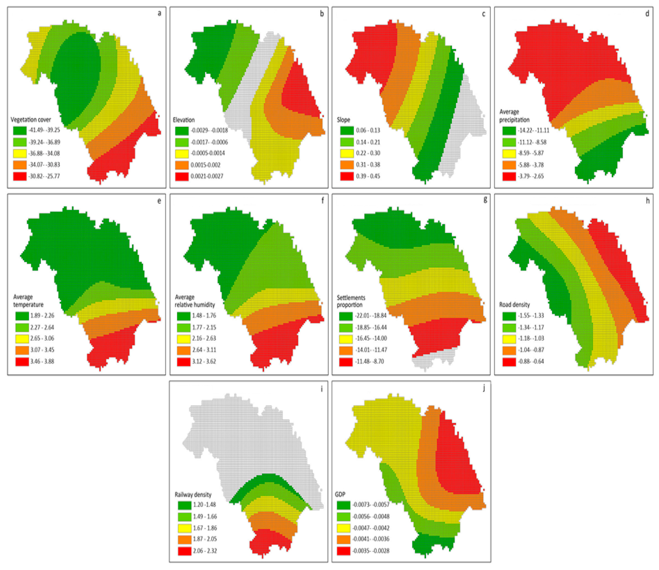
3.1. Comparison of Significant Explanatory Variables between Two Models

Multi-collinearity diagnosis results showed no collinearity between the explanatory variables; thus, they could be used in model fitting for the global NB and GWNBR. Estimated coefficients of the full variables in both models show that slope, railway density, average relative humidity, and average temperature were positively correlated with the occurrence of wildfire; whereas road density, settlement areas, average precipitation, vegetation cover, and GDP were negatively correlated with wildfire occurrence (

Table 2. Coefficient estimates of the full variables models from global negative Binomial (NB) and geographically weighted negative Binomial regression (GWNBR) model.

Statistics	βIntercept	βElevation	βSlope	βRailway density	βRoad density	βSettlement proportion	βAverage relative humidity	βAverage temperature	βAverage precipitation	βVegetation cover	βGDP	βPopulation density
Global negative binominal (NB)
Estimate	−120.6	−0.0002	0.27	0.92	−1.07	−14.63	1.67	1.91	−3.16	−38.15	−0.005	0.0001
Standard deviation	9.4	0.0003	0.03	0.72	0.20	4.47	0.12	0.14	0.54	1.10	0.001	0.0008
Estimate −1Std	−129.9	−0.0005	0.24	0.20	−1.28	−19.10	1.56	1.76	−3.70	−39.25	−0.006	−0.0007
Estimate + 1Std	−111.1	0.0001	0.29	1.64	−0.87	−10.17	1.79	2.05	−2.62	−37.05	−0.004	0.0009
Geographically weighted negative binominal regression (GWNBR)
Minimum value	−275.3	−0.0029	−0.03	−0.79	−1.55	−22.01	1.48	1.89	−14.22	−41.49	−0.007	−0.0012
Lower quartiles	−201.5	−0.001	0.09	0.08	−1.24	−18.47	1.66	2.09	−8.18	−39.42	−0.005	−0.0004
Mean	−161.1	0.0003	0.22	0.82	−1.10	−15.50	2.18	2.48	−5.58	−36.17	−0.004	−0.0001
Media	−142.1	0.001	0.21	0.92	−1.10	−15.97	1.92	2.15	−3.67	−36.86	−0.004	−0.0001
Upper quartiles	−118.5	0.0015	0.35	1.51	−0.94	−12.74	2.68	2.87	−2.97	−33.53	−0.004	0.0002
Maximum value	−106.3	0.0027	0.45	2.32	−0.64	−7.55	3.62	3.88	−2.65	−25.77	−0.003	0.0005

). While the relationship between elevation and fire occurrence was negative in global NB model, it was positive in GWNBR model. Population density showed positive relationship with fire occurrence in global NB model whereas the relationship was negative in GWNBR model. Among 11 explanatory variables, eight variables were significant in global NB model (

Table 3. Model parameter estimation of global negative binominal regression.

Parameters	Estimate	Standard Error	p-Value
Intercept	−120.43	9.53	<0.0001
Slope	0.25	0.02	<0.0001
Road density	−0.96	0.18	<0.0001
Settlement proportion	−14.03	4.22	0.0009
Average relative humidity	1.67	0.12	<0.0001
Average temperature	1.92	0.14	<0.0001
Average precipitation	−3.09	0.56	<0.0001
Vegetation cover	−38.10	1.09	<0.0001
GDP	−0.01	0.001	<0.0001
Dispersion	2.22	0.09

) and 10 variables were significant in GWNBR (Figure 5).

Estimate coefficients of the two models shows that slope, average relative humidity, average temperature were positively correlated with wildfire occurrence in both models, while road density, settlements proportion, average precipitation, vegetation cover, and GDP had a significant negative impact on wildfire occurrence. The relationship between wildfire occurrence and Elevation, Railway density were not significant using the global NB model. In the GWNBR model, the relationship between FVC and fire occurrence is strongest in the middle of the study area; however, there is no significant correlation in the same area (Figure 5a). The influence of elevation in northern and southern parts of the study site on wildfire occurrence was significant (Figure 5b), while railway density had a significant positive impact on wildfires in the southern part of the study site (Figure 5i). There were some areas in the southern part of the study site, where slope (Figure 5c) and settlements proportion (Figure 5g) had no significant effect on the occurrence of wildfires. In addition, the influence of three meteorological variables on the occurrence of forest fire has an obvious difference from south to north (Figure 5d–f). The localized significant factors indicated that the GWR models were capable of targeting and specifying details location by location than the global NB models.

3.2. Comparison of Model Fitting between GWNBR and Global NB

Compared with the global NB model fitted on all variables, the AIC, BIC, and MSE values of GWNBR were smaller, and the spatial autocorrelation results of model residual showed that the Moran’s Index of GWNBR was smaller than the global NB model (

Table 4. Statistics of model fitting and residuals for the global NB and geographically weighted regression (GWR) models with all variables and significant variables.

	All variables		Significant Variables
Statistics	Global NB	GWNBR	Global NB	GWNBR
AIC (Akaike information criterion)	29442.17	22582.42	30138.93	23576.01
BIC (Bayesian Information Criterion)	29959.05	22609.66	30172.17	22760.81
Prediction Accuracy	62.99%	68.23%	62.4%	68.6%
MSE (Mean Square Error)	348.21	82.65	363.04	100.58
Mean of absolute residuals	5.94	2.77	5.9598	2.8911
Std of Residuals	18.56	9.04	18.9521	9.9755
Moran’s Index	0.042	0.02	0.041	0.0204
Z-score	118.2	56.3	114.5	57.3
P-value	<0.0001	<0.0001	<0.0001	<0.0001

). For models fitted on significant variables, the AIC, BIC, MSE, and Moran’s I of the GWNBR model were smaller than the global NB model (Table 4); indicating that applying the GWR approach to locally model the count response variable would improve the model fitting over the global NB models. Figure 4 indicated that the prediction accuracy of GWNBR, either based on all variables or significant variables, was higher than that of global NB.

3.3. Spatial Autocorrelation of Residuals

The Moran’s I of residuals from both global NB and GWNBR models showed the existence of significant positive spatial correlation of the model residuals (Table 4). The results also showed that the relationships between wildfire counts and predictor variables were spatially non-stationary (

Table 5. The interquartile range (IQR) of the GWNBR coefficient estimates with the standard error (SE) of the global NB estimates, indicating spatial non-stationary in the relationships between response variable and its accompanying predictor variables.

Coefficient	IQR(GWR)	SE (Global NB)	2SE (Glzobal NB)	Status
Intercept	83.07	9.41	18.83	Non-stationary
Elevation	0.002	0.0003	0.001	Non-stationary
Slope	0.26	0.03	0.06	Non-stationary
Railway density	1.43	0.72	1.44	Stationary
Road density	0.29	0.20	0.41	Stationary
Settlement proportion	5.74	4.47	8.94	Stationary
Average relative humidity	1.02	0.12	0.23	Non-stationary
Average temperature	0.78	0.14	0.29	Non-stationary
Average precipitation	5.20	0.54	1.08	Non-stationary
Vegetation cover	5.89	1.10	2.20	Non-stationary
GDP	0.001	0.001	0.002	Stationary
Population density	0.001	0.001	0.002	Stationary
Dispersion	0.61	0.09	0.1724	-

). Among explanatory variables considered in this study, elevation, slope, average relative humidity, average temperature, average precipitation, and vegetation cover were non-stationary, while railway density, road density, settlements proportion, GDP, and population density were relatively spatially stationary.

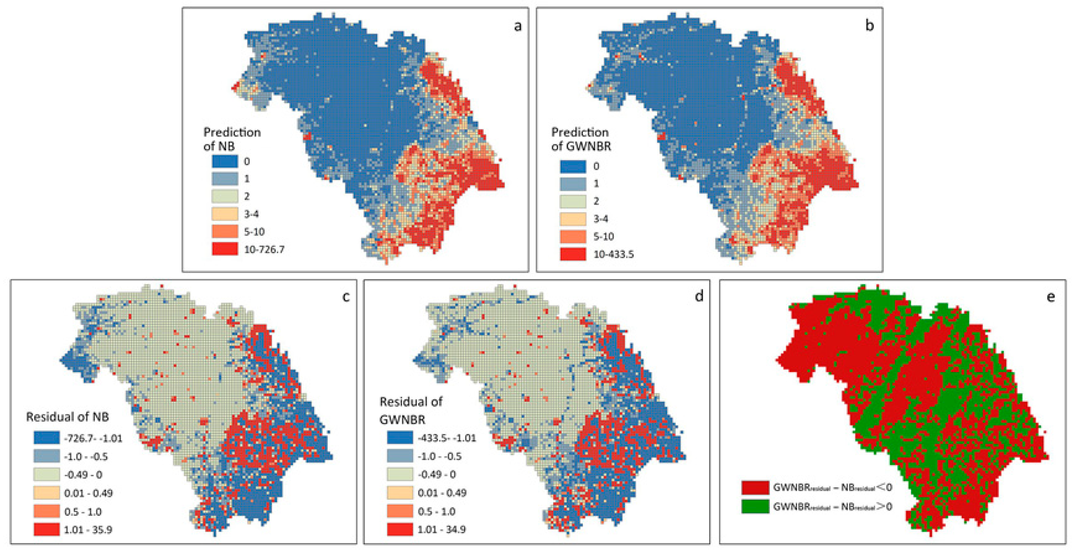
3.4. Spatial Distribution of Fire Occurrence and Residual

The spatial prediction of fire occurrence by the global NB was between 0 and 727, showing that the wildfire did not have full-area coverage, with up to 727 fires occurring in the grid cells (Figure 6a). The model prediction from GWNBR showed narrower range than the global NB model (Figure 6b). More specifically, the prediction of low-value fire points was similar to the global NB model, and fire prediction in some places would not exceed 434 counts at most. The spatial patterns of the model predictions were similar for global NB and GWNBR model. The predicted fire occurrences between 4.5 and the maximum were mostly clustered in the south, east and southeastern region of the Great Xing’an Mountain. The residual maps (Figure 6c,d) show that the predictions were lower than the actual observations in some parts of the southeastern and east of the Great Xing’an Mountains; i.e., these areas were underestimated. Furthermore, we compared the absolute residuals of the global NB and GWNBR, and the absolute residual of GWNBR was smaller than that of global NB (Figure 6e). The red regions in Figure 6e constituted 58.7% of the study area and the prediction by GWNBR in these areas was closer to the true value than the global NB. On the contrary, the green areas (occupy roughly 41.3% of the whole area) showed the prediction by the global NB was closer to the true value than that by the GWNBR.

4. Discussion

The study demonstrates that fire occurrence and its drivers in the Great Xing’an Mountains are spatial variables, and the GWNBR model describes this variability better than the global NB. The GWNBR model has better fitting than non-spatial NB model, with small spatial residuals (Table 2). This is indeed expected as the GWNBR model estimates the local parameters of each unit, which can effectively explain spatial variability [39]. Our result is in line with previous studies that reported better fitting with GWR approach than a non-spatial regression model [6,26]. The results also show that the spatial variability in fire occurrence in the Great Xing’an Mountains is induced by topographic and metrological factors. Thus, consider regional variation in environmental conditions is paramount when studying factors that significantly affect the likelihood of fire occurrence, as the same variables may influence wildfire occurrence differently depending on the location and scale of analysis.

Human factors appeared to have no global impact on wildfires in the present study. In some areas, the number of wildfire occurrences was increased with lower road density, settlements proportion, GDP and higher railway density. Human activities were intensively related to the first three factors in the region, indicating that local wildfires have been weakened by human influence in recent years. One possible explanation for this is that the vegetation in remote forests is more continuous, while the fuel closer to urban areas are fragmented. In addition, the concentration of fire-fighting resources outside the area of human activity is low [40]; thus, when fires spread to more remote forests, they will last longer and devastate a larger area. This means that even though fires occur close to roads or settlements, the burnt areas are often non-urban areas, where fires spread after ignition [13]. On the contrary, the positive railway density coefficients implied that as railway increased more fire would occur, which is only significant in the southern region for the GWNBR model (but not significant for global NB model). The likelihood of fire occurrence close to railway tracks is attributed to errant sparks released from the steam engine, fire accidents that occur in trains, incendiarism by smokers travelling by train, and lack of controlled burning activities near the tracks [4].

Slope is a main factor affecting the occurrence of wildfires, and wildfires occur frequently in steep slopes. It is generally believed that the time of soil water retention is short in the steep slope, leading to low moisture content of soil and forest fuel in the steep slope area, which provides conditions for the occurrence of wildfires [14]. There are fewer wildfires in dense vegetation cover in this study. Vegetation cover affects the wildfire by affecting the temperature of the fine fuel on the underlying surface. In areas with high vegetation coverage, the surface temperature is low, which makes it difficult to evaporate for soil moisture, leading to high fuel moisture content, which is not easy to burn [41]. A similar inverse association for the vegetation cover-fire activity in southern part of the Great Xing’an Mountains using geographically weighted logistic regression model was observed [4], which suggests that the spatial variation of forest fuel may not induce the occurrence of local wildfire occurrence [4]. Even if the vegetation cover is dense and accompanied by more human settlements, it is likely that a low level of fire density can occur [42].

Meteorological factors have a significant impact on wildfires and their spatial heterogeneity is quite explicit. There are more fires in areas with lower precipitation, high temperatures, and relative humidity. Our research results show that temperature has a significant positive impact on fire occurrence, which is also supported by the work of others [43,44]. The changes in temperature will bring the changes in fuel moisture, which will have an impact on wildfires. However, the positive relationship between relative humidity and the likelihood of fire occurrence may sound opposite to people’s expectation. One explanation is that relative humidity has no direct impact on fire occurrence, but affects wildfires by affecting the growth of forest vegetation. Higher relative humidity is beneficial to the growth of ground cover vegetation, which further increases the fuel load. The amount of surface fuel load exacerbates the occurrence of wildfires, if it is exposed to situation with high temperature and low rainfall, resulting in a positive relationship between wildfires and relative humidity [45]. Furthermore, in this study, the relative humidity was measured as the daily average over a 16-year period in each grid, with the minimum of 75% and the maximum of 89%. This small range may reduce the impact of relative humidity change to wildfires. When the relative humidity is measured in different scales, the relationship may be different [14].

For modeling a count response variable, people usually start with a Poisson regression, which, however, is criticized for its restrictive assumption of equality of mean and variance, and the underestimation of the standard errors of the Poisson regression model coefficients due to over-dispersion. A better alternative for correcting this over-dispersion problem is to use the negative Binomial regression, because the negative Binomial distribution automatically builds in a dispersion parameter in its distribution function so that the estimation of both model coefficients and their standard errors would be corrected for the over-dispersion in the data [32,33]. In this study, the observed mean of wildfire counts was 2.54 whereas the variance was 5.572 (Table 1), revealing the over-dispersion problem in the data.

In addition, the traditional global NB model assumes that the variables are spatially stable, while the GWNBR model takes into account the spatial heterogeneity of the model variables; i.e., the local parameters are estimated at each data point, especially for highly spatially variable data. The results of this study show that factors affecting the occurrence of wildfires in the Great Xing’an Mountains have noticeable spatial heterogeneity, and the GWNBR model performs better with respect to predicting fire occurrence and accuracy than the global NB model. Our result is consistent with previous studies in which GWR approach was shown to capture spatial variability better than the global models [4,22,29]. On the other hand, for some variables the GWNBR model may not be best suited to make general inference about the relationship between predictor variables and wildfire occurrence. These relationships may be actually global or local changes due to the interaction of variables. Thus, the GWR method may be a good complement to the global spatial regression model [46]. Its powerful ability to account for the local representation of predictors and their interaction with scales makes it useful for wildfire analysis on a large scale.

There are a few caveats in this study. Although GWNBR is an improved regression method for spatial count-based analysis, some concerns still exist. The first issue is the kernel function and bandwidth selection. In this study, we applied the Gaussian kernel function and bandwidths estimated from the variogram of observed response variable to GWNBR models. It is known that the bandwidth has profound impacts on model fitting and the spatial distributions of model predictions and localized coefficients [25,47]. Second, there was no adequate past or current data for some predictors, such as road density or settlements proportion, which likely change over time. Testing model applicability by including fuel factors (e.g., fuel moisture or load) that promote wildfire occurrence would be the focus of future studies. Data collected from different data sources need to be continuously updated for improving wildfire modeling. Addressing these caveats will provide vital information to develop sound wildfire management practices in a changing socioeconomic and environmental landscape.

5. Conclusions

In this study, the traditional global NB model was used along with GWNBR model to explain wildfire occurrence patterns in the Chinese boreal forest. Based on the findings, the following conclusions can be drawn: (1) GWNBR model has a better performance in model prediction accuracy, model residual reduction, and spatial parameter estimation than the global NB model. The global NB approach seems insufficient to fully describe the spatial relationship between wildfire occurrence and potential predictor variables while the spatial relationship provided by GWNBR enhances the explanatory power of the drivers of wildfires, and reveals the spatiality of the influences of wildfire drivers on wildfire; (2) more wildfires occurred with lower road density, settlements proportion, and GDP, lower vegetation cover, and steeper slope. The areas with high temperature, low rainfall, and high relative humidity are also prone to fire; (3) GWNBR can complement the global NB in overcoming the problem of non-stationary variables; and (4) the GWR technique not only identifies different variables (including spatial variables and local variables), but also provides the significance influence region of local variables, and fully gives the spatial difference information of various variables. This will help explain wildfires in different areas, providing valuable information for local forest managers to design improved fire deployment activities. Thus, considering the geospatial information of predictor variables is essential to improve wildfire occurrence modeling in the boreal forest of China.

References

1. Mckenzie, D.; Shankar, U.; Keane, R.E.; Stavros, E.N.; Heilman, W.E.; Fox, D.G.; Riebau, A.C. Smoke consequences of new wildfire regimes driven by climate change. Earth’s Future 2014, 2, 35–59. [Google Scholar] [CrossRef] [Green Version]
2. Guo, F.; Innes, L.J.; Wang, G.; Ma, X.; Sun, L.; Hu, H.; Su, Z. Historic distribution and driving factors of human-caused fires in the Chinese boreal forest between 1972 and 2005. J. Plant Ecol. 2015, 8, 480–490. [Google Scholar] [CrossRef]
3. Wu, Z.; He, H.; Yang, J.; Liu, Z.; Liang, Y. Relative effects of climatic and local factors on fire occurrence in boreal forest landscapes of northeastern China. Sci. Total Environ. 2014, 493, 472–480. [Google Scholar] [CrossRef] [PubMed]
4. Guo, F.; Selvalakshmi, S.; Lin, F.; Wang, G.; Wang, W.; Su, Z.; Liu, A. Geospatial information on geographical and human factors improved anthropogenic fire occurrence modeling in the Chinese boreal forest. Can. J. For. Res. 2016, 46, 582–594. [Google Scholar] [CrossRef] [Green Version]
5. Guo, F.; Wang, G.; Innes, J.L.; Ma, Z.; Liu, A.; Lin, Y. Comparison of six generalized linear models for occurrence of lightning-induced fires in northern Daxing’an Mountains. China J. For. Res. 2016, 27, 379–388. [Google Scholar] [CrossRef]
6. Guo, F.; Su, Z.; Wang, G.; Sun, L.; Tigabu, M.; Yang, X.; Hu, H. Understanding fire drivers and relative impacts in different Chinese forest ecosystems. Sci. Total Environ. 2017, 605, 411–425. [Google Scholar] [CrossRef] [PubMed]
7. Martinez, J.; Vega-Garcia, C.; Chuvieco, E. Human-caused wildfire riskrating for prevention planning in Spain. J. Environ. Manag. 2009, 90, 1241–1252. [Google Scholar] [CrossRef] [PubMed]
8. Niklasson, M.; Granstrom, A. Numbers and sizes of fires: Long-term spatially explicit fire history in a Swedish boreal landscape. Ecology 2000, 81, 1484–1499. [Google Scholar] [CrossRef]
9. Oliveira, S.; Oehler, F.; San-Miguel-Ayanz, J.; Camia, A.; Pereira, J.M.C. Modeling spatial patterns of fire occurrence in Mediterranean Europe using Multiple Regression and Random Forest. For. Ecol. Manag. 2012, 275, 117–129. [Google Scholar] [CrossRef]
10. Pradhan, B.; Suliman, M.D.H.B.; Awang, M.A.B. Forest fire susceptibility and risk mapping using remote sensing and geographical information systems (GIS). Disaster Prev. Manag. 2007, 16, 344–352. [Google Scholar] [CrossRef]
11. Wallenius, T.H.; Kuuluvainen, T.; Vanha-Majamaa, I. Fire history in relation to site type and vegetation in Vienansalo wilderness in eastern Fennoscandia, Russia. Can. J. For. Res. 2004, 34, 1400–1409. [Google Scholar] [CrossRef]
12. Pereira, M.G.; Trigo, R.M.; da Camara, C.C.; Pereira, J.M.C.; Leite, S.M. Synoptic patterns associated with large summer forest fires in Portugal. Agric. For. Meteorol. 2005, 129, 11–25. [Google Scholar] [CrossRef]
13. Syphard, A.D.; Radeloff, V.C.; Keuler, N.S.; Taylor, R.S.; Hawbaker, T.J.; Stewart, S.I.; Clayton, M.K. Predicting spatial patterns of fire on a southern California landscape. Int. J. Wildland Fire 2008, 17, 602–613. [Google Scholar] [CrossRef]
14. Hu, H. Forest Fire Ecology and Management, 2nd ed.; China Forestry Publishing House: Beijing, China, 2005; p. 66. [Google Scholar]
15. Mandallaz, D.; Ye, R. Prediction of forest fires with Poisson model. Can. J. For. Res. 1997, 27, 1685–1694. [Google Scholar] [CrossRef]
16. Griffith, D.A.; Haining, R. Beyond mule kicks: the Poisson distribution in geographical analysis. Geogr. Anal. 2006, 38, 123–139. [Google Scholar] [CrossRef]
17. Podur, J.J.; Martell, D.L.; Stanford, D. A compound Poisson model for the annual area burned by forest fires in the province of Ontario. Environmetrics 2009, 21, 457–469. [Google Scholar] [CrossRef]
18. Cameron, A.C.; Trivedi, P.K. Regression Analysis of Count Data; Cambridge University Press: Cambridge, UK, 1998. [Google Scholar]
19. Anselin, L.; Griffith, D.A. Do spatial effects really matter in regression analysis? Pap. Reg. Sci. 1988, 65, 11–34. [Google Scholar] [CrossRef]
20. Foody, G.M. Geographical weighting as a further refinement to regression modelling: an example focused on the NDVI-rainfall relationship. Remote Sens. Environ. 2003, 88, 283–293. [Google Scholar] [CrossRef]
21. Wang, Q.; Ni, J.; Tenhunen, J. Application of a geographically-weighted regression analysis to estimate net primary production of Chinese forest ecosystems. Glob. Ecol. Biogeogr. 2005, 14, 379–393. [Google Scholar] [CrossRef]
22. Koutsias, N.; Martínez, J.; Chuvieco, E.; AlligÖwer, B. Modeling wildland fire occurrence in southern Europe by a geographically weighted regression approach. In Proceedings of the 5th International Workshop on Remote Sensing and GIS Applications to Forest Fire Management: Fire Effects Assessment, Zaragoza, Spain, 16–18 June 2005; pp. 57–60. [Google Scholar]
23. Padilla, M.; Vega-Garcia, C. On the comparative importance of fire danger rating indices and their integration with spatial and temporal variables for predicting daily human-caused fire occurrences in Spain. Int. J. Wildland Fire 2011, 20, 46–58. [Google Scholar] [CrossRef]
24. Chuvieco, E.; Aguado, I.; Yebra, M.; Nieto, H.; Salas, P.J.; Martín, M.P. Development of a framework for fire risk assessment using remote sensing and geographic information system technologies. Ecol. Model. 2010, 221, 46–58. [Google Scholar] [CrossRef] [Green Version]
25. Fotheringham, A.S.; Brunsdon, C.; Charlton, M.E. Geographically Weighted Regression: The Analysis of Spatially Varying Relationships; John Wiley and Sons: New York, NY, USA, 2002. [Google Scholar]
26. Rodrigues, M.; De La Riva, J.; Fotheringham, S. Modeling the spatial variation of the explanatory factors of human-caused wildfires in Spain using geographically weighted logistic regression. Appl. Geogr. 2014, 48, 52–63. [Google Scholar] [CrossRef]
27. Justice, C.O.; Giglio, L.; Korontzi, S.; Owens, J.; Morisette, J.T.; Roy, D.; Descloitres, J.; Alleaume, S.; Petitcolin, F.; Kaufman, Y. The MODIS fire products. Remote Sens. Environ. 2002, 83, 244–262. [Google Scholar] [CrossRef]
28. Faivre, N.; Jin, Y.; Goulden, M.L.; Randerson, J.T. Controls on the spatial pattern of wildfire ignitions in Southern California. Int. J. Wildland Fire 2014, 23, 799. [Google Scholar] [CrossRef]
29. Zhang, H.; Qi, P.; Guo, G. Improvement of fire danger modelling with geographically weighted logistic model. Int. J. Wildland Fire 2014, 23, 1130–1146. [Google Scholar] [CrossRef]
30. Purevdorj, T.; Tateishi, R.; Ishiyama, T.; Honda, Y. Relationships between percent vegetation cover and vegetation indices. Int. J. Remote Sens. 1998, 19, 3519–3535. [Google Scholar] [CrossRef]
31. Gutman, G.; Ignatov, A. The derivation of the green vegetation fraction from noaa/avhrr data for use in numerical weather prediction models. Int. J. Remote Sens. 1998, 9, 1533–1543. [Google Scholar] [CrossRef]
32. McCulloch, C.E.; Searle, S.R. Generalized, Linear and Mixed Models; John Wiley & Sons: New York, NY, USA, 2001; pp. 1–184. [Google Scholar]
33. Myers, R.H.; Montgomery, D.C.; Vining, G.G. Generalized Linear Models; John Wiley & Sons: New York, NY, USA, 2002; pp. 100–194. [Google Scholar]
34. Da Silva, A.R.; Rodrigues, T.C.V. Geographically weighted negative binomial regression-incorporating overdispersion. Stat. Comput. 2014, 5, 769–783. [Google Scholar] [CrossRef]
35. SAS Institute, Inc. STAT 9.4 Users’ Manual; SAS Institute, Inc.: Cary, NC, USA, 2013. [Google Scholar]
36. Burnham, K.P.; Anderson, D.R. Multimodel inference: Understanding AIC and BIC in model selection. Sociol. Method. Res. 2004, 33, 261–304. [Google Scholar] [CrossRef]
37. Bailey, T.C.; Gatrell, A.C. Interactive Spatial Data Analysis; Longman Scientific and Technical: Essex, UK, 1995. [Google Scholar]
38. Chen, V.Y.J.; Deng, W.S.; Yang, T.C.; Matthews, S.A. Geographically weighted quantile regression (GWQR): An application to mortality data. Geogr. Anal. 2012, 44, 134–150. [Google Scholar] [CrossRef]
39. Wu, W.; Zhang, L. Comparison of spatial and non-spatial logistic regression models for modeling the occurrence of cloud cover in northeastern Puerto Rico. Appl. Geogr. 2013, 37, 52–62. [Google Scholar] [CrossRef]
40. Calkin, D.E.; Gebert, K.M.; Jones, J.G.; Neilson, R.P. Forest Service large fire area burned and suppression expenditure trends, 1970–2002. J. For. 2005, 103, 179–183. [Google Scholar] [CrossRef]
41. Gabban, A.; San-Miguel-Ayanz, J.; Viegas, D.X. A comparative analysis of the use of NOAA-AVHRR NDVI and FWI data for forest fire risk assessment. Int. J. Remote Sens. 2008, 29, 5677–5687. [Google Scholar] [CrossRef]
42. Lampin-Maillet, C.; Jappiot, M.; Long, M.; Bouillon, C.; Morge, D.; Ferrier, J.P. Mapping wildland-urban interfaces at large scales integrating housing density and vegetation aggregation for fire prevention in the South of France. J. Environ. Manag. 2010, 91, 732–741. [Google Scholar] [CrossRef] [Green Version]
43. Liu, Z.; Yang, J.; Chang, Y.; Weisberg, P.J.; He, H.S. Spatial patterns and drivers of fire occurrence and its future trend under climate change in a boreal forest of Northeast China. Glob. Chang. Biol. 2012, 18, 2041–2056. [Google Scholar] [CrossRef]
44. Hu, T.; Zhou, G. Drivers of lightning-and human-caused fire regimes in the Great Xing’an Mountains. For. Ecol. Manag. 2014, 329, 49–58. [Google Scholar] [CrossRef]
45. Guo, F.T.; Wang, G.Y.; Su, Z.W.; Liang, H.L.; Wang, W.H.; Lin, F.F.; Liu, A.Q. What drives forest fire in Fujian, China? Evidence from logistic regression and Random Forests. Int. J. Wildland Fire 2016, 25, 505–519. [Google Scholar] [CrossRef]
46. Jetz, W.; Rahbek, C.; Lichstein, J.W. Local and global approaches to spatial data analysis in ecology. Glob. Ecol. Biogeogr. 2005, 14, 97–98. [Google Scholar] [CrossRef] [Green Version]
47. Guo, L.; Ma, Z.; Zhang, L. Comparison of bandwidth selection in application of geographically weighted regression: a case study. Can. J. For. Res. 2008, 38, 2526–2534. [Google Scholar] [CrossRef]
Figure 1. Study area and the distribution of Wildfire Counts.
Forests 10 00377 g001
Figure 2. The logical framework of the study.
Forests 10 00377 g002
Figure 3. Frequency distribution of wildfire occurrences.
Forests 10 00377 g003
Figure 4. Spatial distributions of vegetation cover (a), elevation (b), slope (c), average precipitation (d), average temperature (e), average relative humidity (f), settlement proportion (g), road density (h), railway density (i), GDP (j), and population density (k).
Forests 10 00377 g004
Figure 5. Spatial distributions of the significant estimate coefficients of (a) vegetation cover, (b) elevation, (c) slope, (d) average precipitation, (e) average temperature, (f) average relative humidity, (g) settlement proportion, (h) road density, (i) railway density, (j) GDP of the GWNBR model.
Forests 10 00377 g005
Figure 6. Spatial distributions of the model predictions based on global NB (a) and GWNBR (b) models; residuals from global NB (c) and GWNBR (d) models; and the difference between the absolute residuals of GWNBR and global NB (e).
Forests 10 00377 g006