Analysis of Error Structure for Additive Biomass Equations on the Use of Multivariate Likelihood Function

Abstract

Research Highlights: this study developed additive biomass equations respectively from nonlinear regression (NLR) on original data and linear regression (LR) on a log-transformed scale by nonlinear seemingly unrelated regression (NSUR). To choose appropriate regression form, the error structures (additive vs. multiplicative) of compatible biomass equations were determined on the use of the multivariate likelihood function which extended the method of likelihood analysis to the general occasion of a contemporaneously correlated set of equations. Background and Objectives: both NLR and LR could yield the expected predictions for allometric scaling relationship. In recent studies, there are vigorous debates on which regression (NLR or LR) should apply. The main aim of this paper is to analyze the error structure of a compatible system of biomass equations to choose more appropriate regression. Materials and Methods: based on biomass data of 270 trees for three tree species, additive biomass equations were developed respectively for NLR and LR by NSUR. Multivariate likelihood functions were computed to determine the error structure based on the multivariate probability density function. The anti-log correction factor which kept the additive property was obtained separately using the arithmetic and weighted average of basic correction factors from each equation to assess two model specifications on the comparably original scale. Results: the assumption of additive error structure was well favored for an additive system of three species based on the joint likelihood function. However, the error structure of each component equation calculated from the conditional likelihood function for compatible equations might be different. The performance of additive equations corrected by a weighted average of basic correction factor from each component equation performed better than that of the arithmetic average and held good property of compatibility after corrected. Conclusions: NLR provided a better fit for additive biomass equations of three tree species. Additive equations which confirmed the responding assumption of error structure performed better. The joint likelihood function on the use of the multivariate likelihood function could be used to analyze the error structure of the additive system which was a result of a tradeoff for each component equation. Based on the average of correction factors from each component equation to correct the bias of additive equations was feasible for the hold of additive property, which might lead to a poor correction effect for some component equation.

1. Introduction

Allometric research characterizes the scaling relationship between various response variables and different measures of body size, which has been dominant for many years in a variety of different areas, such as physiology, numerical ecology, and morphology [1,2,3]. Kittredge (1944) [4] described the biomass of tree components with tree dimension variables based on an allometric equation to quantify the tree biomass in the form of $Y=a{X}^b$, where Y is tree component biomass, X is tree dimension variable and a, b respectively represents allometric coefficient and exponent. Up to date, thousands of biomass equations have been developed for various tree species and regions all over the world for the purpose of accurate quantification of forest biomass dealing with carbon reduction and climate change [5,6,7]. However, researchers witness a heated issue recently regarding fitting methods which concentrate largely on the topic, linear regression on log-transformed data (hereafter, LR) with a multiplicative error in arithmetic domain or nonlinear regression on original scale (hereafter, NLR) with an additive error.

For decades, LR was the most commonly adopted pattern in allometric research. The conventional practice is to fit a straight line from log-transformed data using ordinary least square and then to back-transform the resulting equation to yield the estimate on the arithmetic scale [8,9,10,11]. Nonetheless, the effectiveness and accuracy of applying LR have been subject to criticism mainly because of the following aspects: (1) Back-transformation from a straight line fitted to logarithm obtained the geometric means for prediction values instead of arithmetic means, which decreased the estimation on the original scale using direct back-transformation [12,13,14]. Although this bias from anti-logarithm could be modified by a certain form of correction factor [8,11,15], some research argued that using anti-log correction factor might cause overestimation [16,17]. (2) While log-transformation could stabilize the variance, it produced an insidious rotational distort for allometric equations which created a new distribution that differed in a fundamental way from the original scale [18,19]. (3) This nonlinear distort unduly emphasized on small values but compressed large-individual values which led to a poor fit for the end of the curve graphically [20,21,22]. (4) The artificial transformation might cause outliers undetected which made the data favorable [19,22,23]. Generally, the focus of controversy for allometric equations fitted by LR lied in the injudicious use of log-transformation [14,22,24].

NLR, directly fitted to the original data by iteration method for allometric equations, has been broadly used by more and more researchers because of convenient and user-friendly statistical software [25,26,27]. However, heteroscedasticity of arithmetic values fitted by NLR directly is of general occurrence which may fail to satisfy statistical assumptions [13,24]. Nonetheless, researches have shown that heteroscedasticity of observations does not necessarily invalidate the deterministic equation fitted by NLR [28] and even the failure of satisfying the constancy of variance, it performed better than LR which yielded more accurate estimates on the original scale [22,29]. It was worthily noted that a weight factor could address the problem of heteroscedasticity by generalized least square as well as the log-transformation of LR [26]. Nonetheless, the debate on which fitting method (NLR or LR) performs better and which error structure confirms the statistical assumption more appropriately has not subsided.

Xiao et al. [30] and Ballantyne [31] proposed the approach of likelihood analysis to determine the error structure (multiplicative vs. additive) for allometric equations so that the suitable fitting procedure (LR or NLR) could be adopted. Recently, the likelihood analysis has come to be applied in the area of forestry and ecology. Lai et al. [32] used the likelihood analysis to compare the allometry of coarse root biomass from LR and NLR for Castanopsis eyrei (Champ. ex Benth.) Tutch., Schima superba Gardn. et Champ., Pinus massonoana Lamb., and mixed species and concluded the empirical data supported a multiplicative error. Ma and Jiang [33] applied the likelihood analysis to determine the error structure of individual tree volume model for Larix gmelinii (Ruprecht) Kuzeneva. and Pinus sylvestris Linn. var. mongolica Litv. which supported the multiplicative error, but the comparison of model assessment indicated NLR performed better than LR. Dong et al. [34] adopted the likelihood analysis to determine the error structure of compatible or additive biomass equations for three conifer species in Northeast China, which favored the multiplicative error. However, the proposed approach of determination on error structure by Xiao et al. [30] and the following application including additive equations developed by Dong et al. [34] were all based on the one-dimension likelihood function which was considered only appropriate for a single allometric equation. For a compatible system of several equations, there were significant contemporaneous correlations when it was simultaneously estimated. Therefore, the analysis based on the one-dimension likelihood function seems to be unreasonable when it applies to determine the error structure for additive biomass equations.

An additive system of biomass equations ensures the logically equal relationship that the predictions for the components sum to the predictions from a total equation. To achieve the additivity property, there are different methods to develop compatible equations. At first, the total predictions could be obtained simply from the sum of components equations developed independently to ensure the additivity [35,36,37]. Up to date, simultaneous estimation for a system of equations widely known as seemingly unrelated regression (SUR) has been broadly used for a compatible system of biomass equations [26,34,37,38]. Back-transformation from a straight line (LR) that fits the logarithm to the original scale could introduce the systematic bias. To remove and reduce this bias, researchers have computed different forms of correction factors and compared the corrected effects. However, little information could be provided when the additive biomass equation was developed by LR. Dong et al. [34] used the correction factor separately from each equation to correct the bias of each component, which did not take the additivity property into account. To our knowledge, the correction factor for additive biomass equation has not been reported, which corrects the bias from anti-log transformation and ensures the additivity property at the same time.

Cinnamomum camphora (L.) Presl, Schima superba Gardn. et Champ. and Liquidambar formosana Hance are widely distributed in Southeastern China and are also the dominant broad-leaved tree species in Guangdong province. There are many differences in morphology and physiology between broad-leaved and conifer tree species. But researches on the biomass equations centered mostly on the conifer species while there are limited studies on broad-leaved tree species [6,27,34,39]. The purpose of our study is (1) to develop a compatible system of biomass equations between branch, foliage, stem wood, stem bark and total aboveground for three broad-leaved tree species separately based on NLR and LR by SUR, (2) to compute the multivariate likelihood function for determination on the error structure of additive biomass equations which extend the method of likelihood analysis to the general situation of a contemporaneously correlated set of equations, (3) to formulate the correction factor for a compatible system of biomass equations to correct the bias introduced by anti-logarithm transformation and ensure the additivity property at the same time, (4) to compare the fitting result of two procedures based on NLR and LR on the same arithmetic scale and evaluate the effect of assumption for different error structures on the result of model fitting.

2. Material and Methods

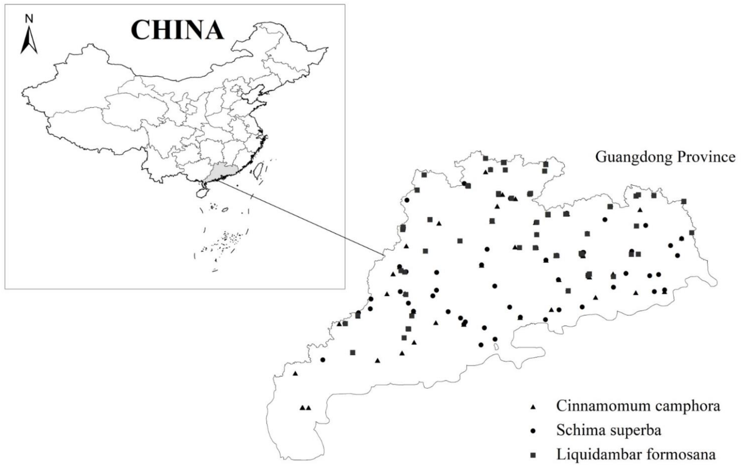
2.1. Data Collection

Tree dimension variable and biomass data, including Cinnamomum camphora, Schima superba and Liquidambar formosana covering whole Guangdong province in Southeastern China with 90 trees for each species, were sampled in 2013 by Guangdong Forestry Survey and Planning Institute (Figure 1). The sample trees were classified by the diameter class of 2 cm, 4 cm, 6 cm, 8 cm, 12 cm, 16 cm, 20 cm, 26 cm, 32 cm and 38 cm (above 38 cm). Among them, 60 trees were evenly distributed following above 10 diameter classes with six trees for each class and the remaining 30 trees were chosen based on the actual distribution of diameter class and the number of trees from the 8th National Forest Inventory in Guangdong province.

The destructive sampling procedure was processed for the living sample trees avoiding severe defects. Before the tree was felled at the ground level height, the diameter at breast height (D, at 1.3 m aboveground) was measured. After felled, the living crown was evenly marked into three parts (top, middle, and bottom) and weighted separately, then the branches and leaves from each part summing to about 500–1000 g of fresh mass was randomly sampled and placed in a labeled bag for moisture content determination. The stem was also marked into three sections including 0–2/10, 2/10–5/10 and above 5/10 tree height and weighed separately. At each section of the stem, a 2–3 cm thick disk separately from the upper and lower part was cut and weighed, then taken to the laboratory for moisture content determination. All samples were dried at 85 °C to constant weight. The dry biomass of each component was calculated by multiplying the fresh weight of each component by the dry/fresh ratio of each component sample. The total foliage biomass was the sum of foliage dry biomass. The total stem wood biomass was the sum of all stem wood’s sections dry mass. The total stem bark biomass is the sum of all stem bark dry mass. The aboveground biomass was the sum of branch, foliage, stem wood, and stem bark dry biomass. The above procedure of moisture content determination was conducted by the laboratory center of College of Forestry and Landscape Architecture, South China Agriculture University according to the related technical regulations [40]. The data statistics were summarized for 90 sampling trees of each broad-leaved species in

Table 1. The descriptive statistics for 90 sampling trees of each broad-leaved tree species.

Variable	Cinnamomum camphora (L.) Presl			Schima superba Gardn. et Champ.			Liquidambar formosana Hance.
	Range	Mean	SD	Range	Mean	SD	Range	Mean	SD
Diameter/cm	1.9–41.0	14.5	10.5	1.7–51.5	14.4	10.9	1.8–43.5	14.4	10.6
Branch/kg	0.1–547.0	44.8	105.1	0.1–371.0	36.3	65.9	0.1–468.7	30.0	62.4
Foliage/kg	0.1–89.8	5.8	12.5	0.1–45.7	5.7	8.7	0.1–46.4	4.6	9.6
Stem wood/kg	0.2–519.7	62.1	100.1	0.3–570.7	69.2	110.5	0.2–569.9	81.5	127.8
Stem bark/kg	0.1–75.5	10.5	16.1	0.1–89.0	12.6	19.5	0.1–121.6	13.1	20.5
Aboveground/kg	0.4–1016.9	123.1	221.7	0.6–897.4	123.8	192.2	0.3–955.5	129.2	206.1

Note: SD was standard deviation.

.

2.2. Model Specification and Estimation

To fit the allometric equation, either NLR on the arithmetic scale or LR on the logarithmic scale could yield the estimation values. The fundamentally substantial difference between these two approaches largely relies on the assumption of how error term manifests in the equation, which is known as the error structure (Xiao et al., 2011) [30]. NLR assumes the equation with the normally additive error on the arithmetic scale such that:

$$Y=a{x}^b+\epsilon ,\hspace{1em}\epsilon ~N\left(0,{\sigma }^2\right)$$

(1)

In contrast, LR assumes that the error is normally distributed and additive on the logarithmic scale such that:

$$\mathit{log}Y=\mathit{log}a+b\mathit{log}x+\epsilon ,\hspace{1em}\epsilon ~N\left(0,{\sigma }^2\right)$$

(2)

which corresponds to log-normally distributed, multiplicative error on the arithmetic scale,

$$Y=a{x}^b\times \exp \left(\epsilon \right),\hspace{1em}\epsilon ~N\left(0,{\sigma }^2\right)$$

(3)

To determine which model specification was the most appropriate for a compatible system of biomass equations for three broad-leaved tree species in this study, two model forms that correlated with additivity among four component biomass equations and total aboveground biomass equation were specified as follows with cross-equation constraints on the structural parameters:

(1) The first model specification assumes the error structure is additive (Equation (1)) and a compatible system of five biomass equations as follows:

$$\begin{gathered} W_{BR}=a_1·D^{b_1}+{\epsilon }_1 \\ {W}_{FL}=a_2·D^{b_2}+{\epsilon }_2 \\ {W}_{SW}=a_3·D^{b_3}+{\epsilon }_3 \\ {W}_{SB}=a_4·D^{b_4}+{\epsilon }_4 \\ {W}_{AB}=a_1·D^{b_1}+a_2·D^{b_2}+a_3·D^{b_3}+a_4·D^{b_4}+{\epsilon }_5 \end{gathered}$$

(4)

(2) The second model specification assumes the error structure is multiplicative on the arithmetic scale (Equation (3)) and logarithmic transformation was taken on both sides of equations (Equation (2)) such that

$$\begin{gathered} log{W}_{BR}=\mathit{log}{a}_1+b_1\mathit{log}D+{\epsilon }_1^{\prime } \\ log{W}_{FL}=\mathit{log}{a}_2+b_2\mathit{log}D+{\epsilon }_2^{\prime } \\ log{W}_{SW}=\mathit{log}{a}_3+b_3\mathit{log}D+{\epsilon }_3^{\prime } \\ log{W}_{SB}=\mathit{log}{a}_4+b_4\mathit{log}D+{\epsilon }_4^{\prime } \\ log{W}_{AB}=\mathit{log}\left(a_1·D^{b_1}+a_2·D^{b_2}+a_3·D^{b_3}+a_4·D^{b_4}\right)+{\epsilon }_5^{\prime } \end{gathered}$$

(5)

where $W_{BR}, W_{FL}, W_{SW}, W_{SB}$ and $W_{AB}$ represent branch biomass, foliage biomass, stem wood biomass, stem bark biomass and the aboveground biomass in kg, respectively, D is the diameter at breast height in cm, log denotes natural logarithm, $a_i$ and $b_i$ are regression coefficient for Equation (4), $\log a_i$ is the intercept and $b_i$ is the regression coefficient for Equation (5), ${\epsilon }_i$ and ${\epsilon }_i^{\prime }$ are the equation error terms for NLR and LR additive model, respectively.

Above two model specifications for additive biomass equations were estimated using nonlinear seemingly unrelated regression generally known as NSUR. The logarithmic transformation tends to balance the heteroscedastic variance. For comparison, Equation (4) was fitted to data using weighted NSUR as demonstrated by Parresol (2001) [26] to stabilize the variance. The weight of each component equation was obtained by the weight function $w=\sqrt{f{\left(D\right)}^{-1}}$, where $f\left(D\right)$ was the prediction value for estimated equation [26,41,42].

2.3. Multivariate Likelihood Function to Analyze Error Structure

Xiao et al. [30] outlined the approach of likelihood analysis to facilitate the objective determination of the error structure based on the single one-dimension likelihood function. When applied to the additive biomass model with cross-equation correlation, it seems. Considering that, in this study, we computed the multivariate likelihood function including the joint likelihood function and the conditional likelihood function to respectively analyze model system and each component equation for the correlated error structure of additive biomass equations. Based on the joint probability density function, the joint likelihood function can be calculated by:

(1) For the p components system of NLR (Equation (4)), the joint likelihood function that the data are generated from a normal distribution with additive error is calculated as follows:

$$L_{NLR}^{\left(p\right)}={{\displaystyle \prod }}_{j=1}^n\left[\frac{1}{{\left(2\pi \right)}^{p∕2}{\left|{\Sigma }_{NLR}\right|}^{1/2}}\exp [-\frac{1}{2}{(w_{ij}·(Y_{ij}-a_{NLR}{X}_{ij}^{b_{NLR}}))}^{\prime }{\Sigma }_{NLR}{}^{-1}(w_{ij}·(Y_{ij}-a_{NLR}{X}_{ij}^{b_{NLR}}))]\right]$$

(6)

(2) For the p components system of LR (Equation (5)), the joint likelihood function that the data are generated from a lognormal distribution with multiplicative error on the arithmetic scale:

$$L_{LR}^{\left(p\right)}={{\displaystyle \prod }}_{j=1}^n\left[\frac{1}{y_i·{\left(2\pi \right)}^{p∕2}{\left|{\Sigma }_{LR}\right|}^{1/2}}\exp [-\frac{1}{2}{(\log Y_{ij}-\log (a_{LR}{X}_{ij}^{b_{LR}}))}^{\prime }{\Sigma }_{LR}{}^{-1}(\log Y_{ij}-\log (a_{LR}{X}_{ij}^{b_{LR}}))]\right]$$

(7)

where $L_{NLR}^{\left(p\right)}$, $L_{LR}^{\left(p\right)}$ are the joint likelihood function of NLR and LR for p component equations, respectively. Where n is the sample size. $X_{ij}, Y_{ij}$ (i = 1, …, p; j = 1, …, n) are the jth value for predictor and response variable of the ith component equation, respectively. ${\Sigma }_{NLR}$, ${\Sigma }_{LR}$ are the error variance-covariance matrix of NLR and LR, respectively. $\left|{\Sigma }_{NLR}\right|$, $\left|{\Sigma }_{LR}\right|$ are the determinant of responding matrix respectively, $w_{ij}$ is the weight of the jth predicted value of the ith component equation. $a_{NLR}$, $b_{NLR}$, $b_{NLR}$ and $b_{LR}$ are the responding regression coefficient for NLR and LR, respectively.

According to the definition of conditional distribution for the multivariate probability density function [43], the conditional likelihood function for ith component equation can be defined as follows:

$$L_{NLR}\left(L_{NLR}^{\left(i\right)}|L_{NLR}^{\left(p-i\right)}\right)=L_{NLR}^{\left(p\right)}/L_{NLR}^{\left(p-i\right)}$$

(8)

$$L_{LR}\left(L_{LR}^{\left(i\right)}{|L}_{LR}^{\left(p-i\right)}\right)=L_{LR}^{\left(p\right)}/L_{LR}^{\left(p-i\right)}$$

(9)

where $L_{NLR}\left(L_{NLR}^{\left(i\right)}|L_{NLR}^{\left(p-i\right)}\right)$, $L_{LR}\left(L_{LR}^{\left(i\right)}{|L}_{LR}^{\left(p-i\right)}\right)$ is the conditional likelihood function for ith component equation of NLR and LR respectively, $L_{NLR}^{\left(i\right)}$, $L_{LR}^{\left(i\right)}$ is the likelihood function for ith component equation of NLR and LR respectively. $L_{NLR}^{\left(p-i\right)}$, $L_{LR}^{\left(p-i\right)}$ is the value of the joint likelihood function calculated from (p − i) components without the use of ith component equation for NLR and LR, respectively.

To compare different candidate models fitted to the same dataset statistically, Akaikes’s Information Criterion (AIC) can be used to evaluate the goodness-of-fit of a model by involving both the likelihood and a penalty for extra parameters. The lowest value for AIC identifies the candidate model conveying the most information about the relationship between predictor and response. AIC_c which is a second-order variant of AIC for small sample size is computed as

$$AI{C}_c=2k-2\mathit{log}L+\frac{2k\left(k+1\right)}{n-k-1}$$

(10)

where k is the number of parameters. L is the joint likelihood function for the model system (Equation (6) for NLR and Equation (7) for LR) or the conditional likelihood function for each component equation (Equation (8) for NLR and Equation (9) for LR). If $AI{C}_{c-norm}-AI{C}_{c-logn}<-2$, the assumption of additive error is favored and the result from Equation (4) should be processed. If $AI{C}_{c-norm}-AI{C}_{c-logn}>2$, the assumption of multiplicative error is favored and the result from Equation (5) should be processed [44]. If $\left|AI{C}_{c-norm}-AI{C}_{c-logn}\right|\le 2$, neither of these two error structures is appropriate and model averaging is suggested. Besides the difference of AIC respectively from NLR and LR, evidence ratio (ER) (see Appendix A) was also taken to provide the evidence for the appropriate model selection [44].

2.4. Back-Transformed Correction Factor for Additive Equations

To obtain the arithmetic value of prediction, a correction factor (hereafter, CF) is commonly used to correct the systematic bias introduce by anti-log transformation from a straight line (Equation (2)) fitted to logarithmic data. For the additively log-transformed biomass equations (Equation (5)), not only the systematic bias should be corrected, but also the additivity property of the value of prediction from back-transformation need to be satisfied. Thus, based on the basic CF, we formulated the specific correction factor for a compatible system of biomass equations. The two basic CFs for ith component can be calculated as follows [8,15]:

$$C{F}_{i1}=\mathit{exp}\left({\delta }_{ii}^2/2\right)$$

(11)

$$C{F}_{i2}={{\displaystyle \sum }}_{j=1}^n{y}_{ij}/{{\displaystyle \sum }}_{j=1}^n{\widehat{y}}_{ij}$$

(12)

where ${\delta }_{ii}^2$ is the ith diagonal element of the error variance-covariance matrix, $y_{ij}$ is the jth observed value for ith component, ${\widehat{y}}_{ij}$ is the predicted value of the jth observed value for ith component. Then, the arithmetic and weighted average CF for the compatible system can be respectively obtained by

$$C{F}_{at}=\frac{1}{p}{{\displaystyle \sum }}_{i=1}^{p}C{F}_{it} t=1, 2$$

(13)

$$C{F}_{wt}=\frac{1}{2}{{\displaystyle \sum }}_{i=1}^p{W}_i·C{F}_{it} t=1, 2$$

(14)

where $C{F}_{at}$, $C{F}_{wt}$ are the arithmetic and weighted average of the tth (t = 1, 2) basic correction factor from each component equation, respectively. $C{F}_{it}$ is the tth (t = 1, 2) basic correction factor for ith component equation, $W_i$ is the proportion of the ith component biomass accounted for the total aboveground biomass.

2.5. Model Assessment

This study used the entire empirical data to fit additive biomass equations [45]. Model fitting and predicting was assessed by the statistics as follows.

Coefficient of determination

$$R^2=1-{{\displaystyle \sum }}_{j=1}^n{\left(y_j-{\widehat{y}}_j\right)}^2/{{\displaystyle \sum }}_{j=1}^n{\left(y_j-\overline{y}\right)}^2$$

(15)

Standard error of estimate

$$SEE=\sqrt{\frac{1}{n-k}{{\displaystyle \sum }}_{j=1}^n{\left(y_j-{\widehat{y}}_j\right)}^2}$$

(16)

Total relative error

$$TRE={\displaystyle \sum }_{j=1}^n\left(y_j-{\widehat{y}}_j\right)/{\displaystyle \sum }_{j=1}^n{\widehat{y}}_j\times 100\%$$

(17)

Average system error

$$ASE=\frac{1}{n}{\displaystyle \sum }_{j=1}^n\left[\left(y_j-{\widehat{y}}_j\right)/{\widehat{y}}_j\right]\times 100\%$$

(18)

Relatively mean absolute error

$$RMA=\frac{1}{n}{\displaystyle \sum }_{j=1}^n\left|\left(y_j-{\widehat{y}}_j\right)/{\widehat{y}}_j\right|\times 100\%$$

(19)

Mean prediction error

$$MPE=t_{\alpha }·\left(SEE/\overline{y}\right)/\sqrt{n}\times 100\%$$

(20)

where $y_j$, ${\widehat{y}}_j$ are the jth observed value and the responding predicted value, $\overline{y}$ is the average of the observed value, k is the number of parameters, $t_{\alpha }$ is the t value when the confidence level is α (usually taken by 95%).

To ensure that the estimated mean function captures dominant pattern in the arithmetic scale, the fitted model not only needs to be assessed by several statistics but also should be validated graphically, which was a critically important oversight by many researchers [23,46]. In this study, the additive biomass equations based on different assumptions of error structure (additive vs. multiplicative) were validated graphically.

3. Result

3.1. Error Structure for Each Component Equation and Additive System

Additive biomass equations were fitted to original and log-transformed data, respectively (Equation (4) and Equation (5)), to yield the parameter estimation value, then calculated the AIC_c, respectively, namely AIC_c-norm for Equation (4) and AIC_c-logn for Equation (5) based on the conditional likelihood function from the conditional probability density function. The difference between AIC_c value and parameter estimate were computed in

Table 2. Results of parameter estimate and likelihood analysis based on conditional.

Species	Component	$\Delta \mathbf{A}\mathbf{I}{\mathbf{C}}_{\mathbf{c}}$	ER	LR			NLR
				a	b	$\mathbf{A}\mathbf{I}{\mathbf{C}}_{\mathbf{c}-\mathbf{logn}}$	a	b	$\mathbf{A}\mathbf{I}{\mathbf{C}}_{\mathbf{c}-\mathbf{norm}}$
Cinnamomum camphora	Branch	38.3	<<10−2	0.01231 (0.00218)	2.74507 (0.06317)	357.8	0.01213 (0.00197)	2.75077 (0.05655)	396.1
	Foliage	263.2	<<10−2	0.01429 (0.00356)	2.04953 (0.09561)	228.3	0.01360 (0.00246)	2.09921 (0.07636)	491.5
	Stem wood	−55.5	>>102	0.07100 (0.00741)	2.26782 (0.03982)	350.8	0.08086 (0.02089)	2.26358 (0.07766)	295.3
	Stem bark	−15.9	>>102	0.02016 (0.00307)	2.0898 (0.05842)	216.5	0.03274 (0.01061)	1.99888 (0.09682)	200.6
	Aboveground	−105.6	>>102	—	—	396.1	—	—	290.5
Schima superba	Branch	−495.5	>>102	0.03682 (0.00596)	2.37522 (0.06300)	340.0	0.05756 (0.01954)	2.18189 (0.10335)	−155.5
	Foliage	−263.2	>>102	0.07793 (0.01242)	1.44971 (0.07602)	276.3	0.04990 (0.01759)	1.66296 (0.11131)	13.1
	Stem wood	−530.9	>>102	0.08755 (0.00892)	2.24571 (0.04176)	317.8	0.14024 (0.02612)	2.13536 (0.05512)	−213.1
	Stem bark	−311.7	>>102	0.02301 (0.00295)	2.13066 (0.05245)	253.0	0.04092 (0.01291)	1.9895 (0.09415)	−58.7
	Aboveground	−617.1	>>102	—	—	364.8	—	—	−252.3
Liquidambar formosana	Branch	−595.5	>>102	0.01603 (0.00312)	2.51909 (0.07487)	357.3	0.01702 (0.00551)	2.51466 (0.10100)	−238.2
	Foliage	−221.5	>>102	0.00385 (0.00117)	2.26453 (0.12098)	167.8	0.00475 (0.00219)	2.33859 (0.13845)	−53.7
	Stem wood	−670.7	>>102	0.08077 (0.00991)	2.33577 (0.04822)	347.8	0.09299 (0.01878)	2.30736 (0.06021)	−322.9
	Stem bark	−401.6	>>102	0.02048 (0.00310)	2.19051 (0.05960)	238.5	0.02329 (0.00480)	2.17340 (0.06284)	−163.1
	Aboveground	−731.2	>>102	—	—	379.6	—	—	−351.6

Note: Values in parentheses are the standard error of the mean. ${\Delta \mathrm{AIC}}_{\mathrm{c}}={\mathrm{AIC}}_{\mathrm{c}-\mathrm{norm}}-{\mathrm{AIC}}_{\mathrm{c}-\mathrm{logn}}$. ${\mathrm{AIC}}_{\mathrm{c}-\mathrm{norm}}$ was AIC value calculated from the nonlinear regression model and ${\mathrm{AIC}}_{\mathrm{c}-\mathrm{logn}}$ was AIC value calculated from the linear regression model. NLR and LR represents the nonlinear and linear regression respectively. ER represents the evidence ratio. The symbol “<<” and “>>” denotes far less than and far greater than.

. The AIC_c-norm for Schima superba and Liquidambar formosana was clearly lower than AIC_c-logn with a difference between −731.2 and −221.5 supporting the additive error for each component equation. But there existed different error structures for each component equation of Cinnamomum camphora. The AIC_c-norm for branch and foliage was larger than AIC_c-logn favoring the multiplicative error structure with a difference of 38.3 and 263.2 while for other component equation, the AIC_c-norm was lower than AIC_c-logn with a difference between −105.9 and −15.9 favoring the additive error structure. Components for two other tree species had a large ER (evidence ratio) more than 100 supporting the additive error as well, while the branch and foliage for Cinnamomum camphora had a smaller ER less than 0.01 supporting the multiplicative error as well.

The joint likelihood function was calculated for the whole model system based on the joint probability density function. The analysis of error structure for additive model system was shown in

Table 3. Results of likelihood analysis based on the joint likelihood function for additive system of three tree species.

Species	${\Delta \mathbf{AIC}}_{\mathbf{c}}$	ER	LR		NLR
			${\mathbf{logL}}_{\mathbf{LR}}$	${\mathbf{AIC}}_{\mathbf{c}-\mathbf{logn}}$	${\mathbf{logL}}_{\mathbf{NLR}}$	${\mathbf{AIC}}_{\mathbf{c}-\mathbf{norm}}$
Cinnamomum camphora	−7.0	33	−961.8	1941.3	−958.3	1934.3
Schima superba	−810.2	>>102	−1018.0	2053.8	−612.9	1243.6
Liquidambar formosana	−846.7	>>102	−952.4	1922.6	−529.1	1075.9

. The AIC_c-norm for three tree species was all lower than AIC_c-logn with a difference of −7.0, −810.2 and −846.7 and got relatively large ER as well, supporting the additive error, which meant that the approach of NLR for additive biomass equations was appropriate for three broad-leaved tree species, especially for Schima superba and Liquidambar formosana in this study.

3.2. Assessment of Anti-Log Correction Factor for Additive System

Log-transformed equation predicts the logarithm of the response variable. To obtain the unbiased value in the original scale, the anti-log correction factor is necessary. The arithmetic and weighted average ($C{F}_{at}$ and $C{F}_{wt}$) of basic correction factors from each equation as well as responding evaluation statistics for total aboveground biomass was listed in

Table 4. Evaluation statistics of aboveground biomass applying different correction factors for three tree species.

Species	Model	Basic CF	Additive Model CF	CF Value	R2	SEE	TRE	ASE	RMA	MPE
Cinnamomum camphora	NLR	-	-	-	0.897	73.14	1.36	−5.52	17.92	10.22
	LR	CF0	-	1.00000	0.880	78.91	9.62	4.38	19.35	11.02
		CF1	${\mathrm{CF}}_{a1}$	1.13975	0.905	70.25	−3.82	−8.42	18.17	9.81
			${\mathrm{CF}}_{\mathrm{W}1}$	1.07544	0.898	72.84	1.93	−2.94	17.83	10.18
		CF2	${\mathrm{CF}}_{a2}$	1.11111	0.903	71.08	−1.35	−6.06	17.82	9.93
			${\mathrm{CF}}_{\mathrm{W}2}$	1.09824	0.901	71.63	−0.19	−4.96	17.76	10.01
Schima superba	NLR	-	-	-	0.903	60.32	0.92	−6.65	21.71	8.54
	LR	CF0	-	1.00000	0.890	64.15	2.61	5.72	21.61	9.08
		CF1	${\mathrm{CF}}_{a1}$	1.12639	0.849	75.06	−8.90	−6.15	19.86	10.63
			${\mathrm{CF}}_{\mathrm{W}1}$	1.06502	0.875	68.42	−3.65	−0.74	20.05	9.69
		CF2	${\mathrm{CF}}_{a2}$	1.08285	0.868	70.11	−5.24	−2.37	19.88	9.93
			${\mathrm{CF}}_{\mathrm{W}2}$	1.03248	0.884	65.88	−0.62	2.39	20.68	9.33
Liquidambar formosana	NLR	-	-	-	0.933	53.85	0.23	−2.77	19.79	7.31
	LR	CF0	-	1.00000	0.929	55.42	6.54	5.30	21.05	7.52
		CF1	${\mathrm{CF}}_{a1}$	1.17647	0.915	60.36	−9.44	−10.5	20.32	8.19
			${\mathrm{CF}}_{\mathrm{W}1}$	1.08010	0.932	54.18	−1.36	−2.51	19.67	7.36
		CF2	${\mathrm{CF}}_{a2}$	1.16312	0.919	59.06	−8.40	−9.47	20.12	8.02
			${\mathrm{CF}}_{\mathrm{W}2}$	1.06842	0.932	53.99	−0.28	−1.45	19.71	7.33

Note: CF is correction factor. SEE is standard error of estimate (see Equation (16)). TRE is total relative error (see Equation (17)). ASE is average system error (see Equation (18)). RMA is relatively mean absolute error (see Equation (19)). MPE is mean prediction error (see Equation (20)).

. The arithmetic average of basic CF from each component equation was represented by $C{F}_{at}$ (t = 1, 2) and the weighted average of basic CF from each component equation was represented by $C{F}_{wt}$ (t = 1, 2). CF₀ represented the model was not corrected.

The uncorrected model performed worse with a lower R², larger standard error of estimate (SEE, hereafter) and mean prediction error (MPE, hereafter) than that of NLR for three tree species. Thus, NLR model could yield relatively better prediction compared to the uncorrected LR model. After applying the CF for Cinnamomum camphora, R² of LR model improved by 0.018 to 0.025, SEE decreased by 6.07 kg to 8.66 kg and total relative error (TRE, hereafter), Relatively mean absolute error (RMA, hereafter) and MPE dropped in varying degrees. Importantly, R² and SEE might not be the best with $C{F}_{w2}$, but the remaining statistics including TRE, average system error (ASE, hereafter), RMA, and MPE were even better than NLR. LR model for Schima superba obtained worse fitting and predicting accuracy when it was corrected with R² decreasing by 0.006 to 0.041 and SEE increasing by 1.73 kg to 10.91 kg, but among the different four CFs, the correction effect for $C{F}_{w2}$ was relatively better than that of other correction factors, and TRE, ASE and RMA statistics was better than that of NLR model. The different assessment statistics of corrected LR model got dropped and increased to different degrees for Liquidambar formosana. Using $C{F}_{w2}$ increased the R² by 0.003, dropped the SEE by 1.43 kg compared with LR₀, and the ASE and RMA statistics was better than NLR model, but in terms of R² and SEE statistics, it was slightly worse than NLR model.

$C{F}_{wt}$ (t = 1, 2) corrected better for Schima superba and Liquidambar formosana especially the CF based on secondly basic correction factor (Equation (12)), that is $C{F}_{w2}$. Although $C{F}_{at}$ could yield higher R², TRE and ASE got relatively larger and reached −3.82%, −1.35% and −8.42%, −6.06%, respectively. Generally speaking, the value of $C{F}_{wt}$ was larger than that of $C{F}_{at}$. The approach of weighted average apparently reduced TRE and ASE for additive biomass equations. Taking Liquidambar formosana as an example, based on two basic CFs using the approach of weighted average, TRE reduced by 8.08% and 8.12% while ASE reduced 7.99% and 8.02%. As far as all the evaluation statistics, $C{F}_{w2}$ corrected best for aboveground biomass of additive equations for three broad-leaved tree species. When CF_w2 for additive system was used, it did not perform better than NLR model except Cinnamomum camphora which is slightly better than NLR, but the difference between NLR and corrected LR model was small for three tree species total aboveground biomass.

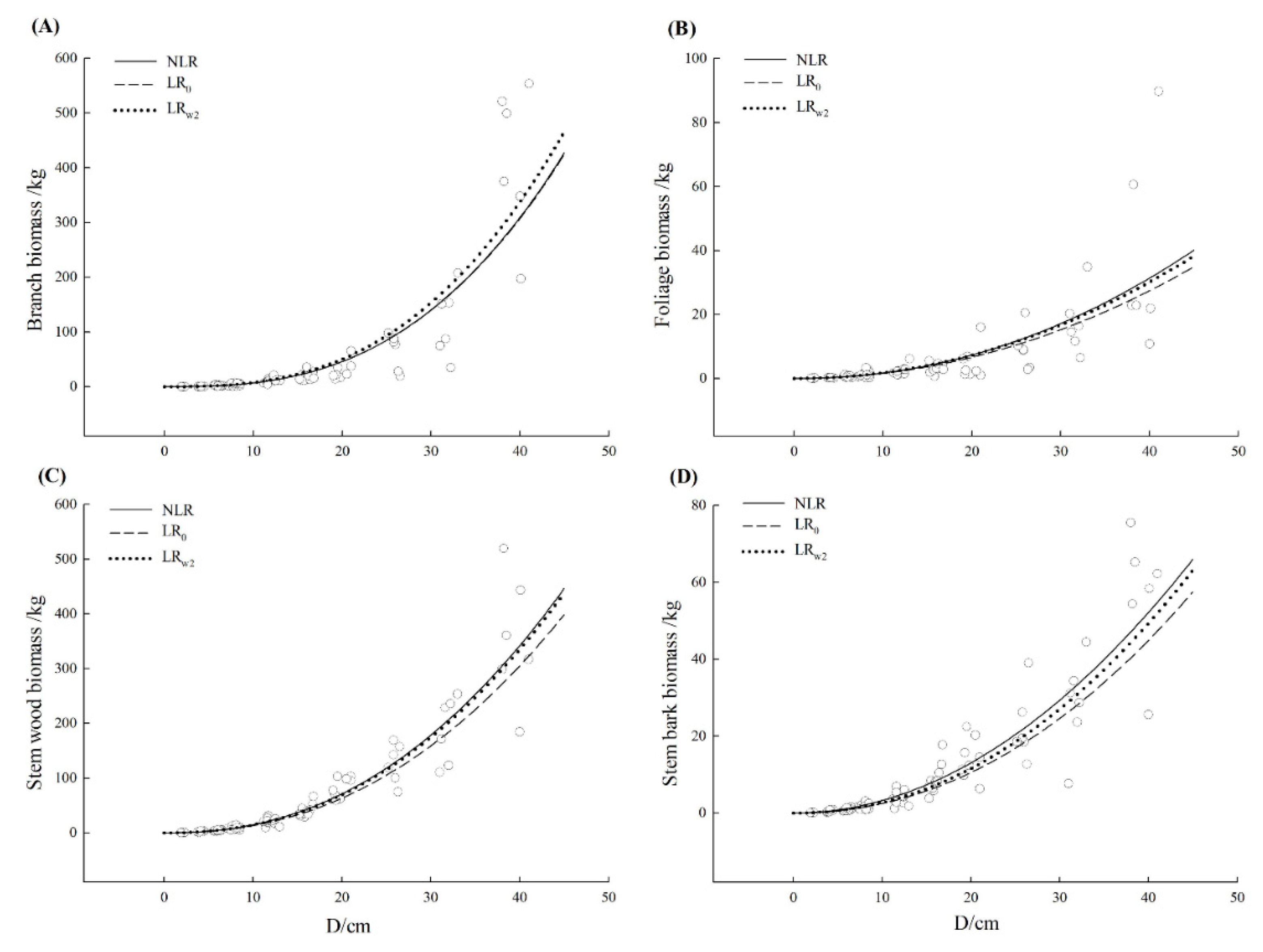
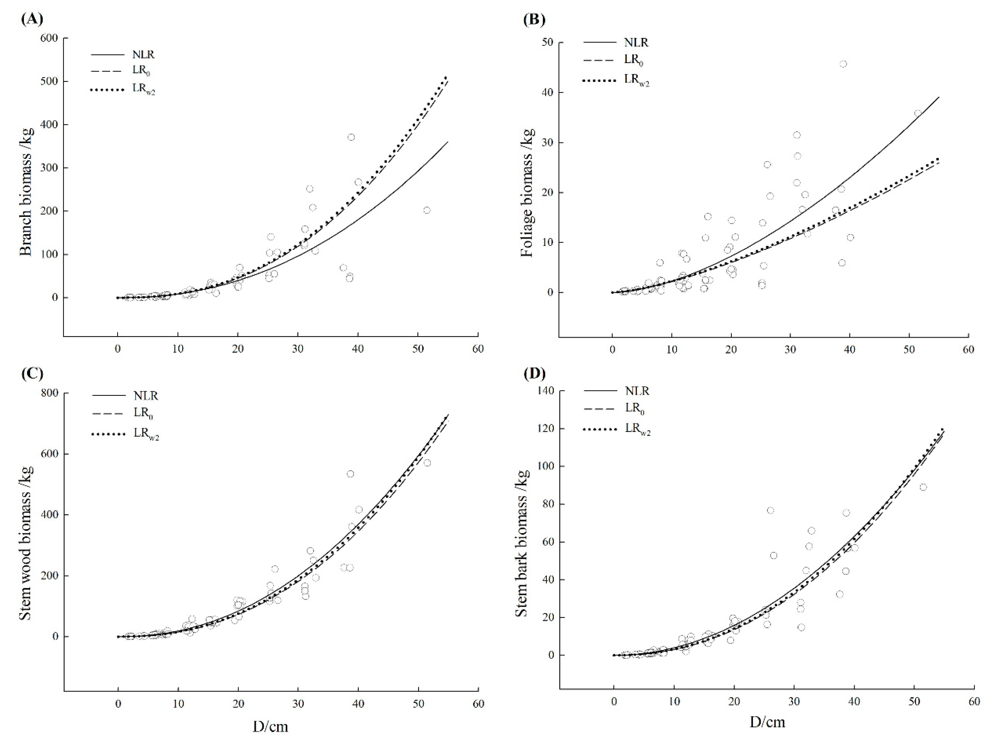
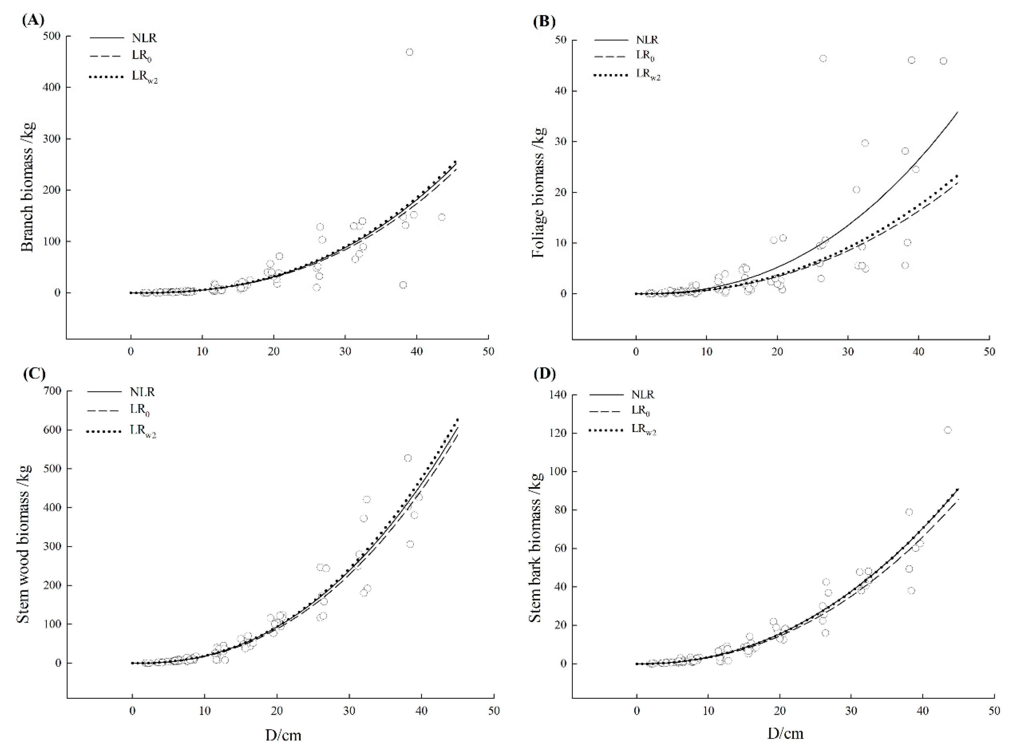
3.3. Comparison of Model Fitting and Error Structure

Major violation indicated the inappropriateness of the model and potential invalidity of the result. To assess the correction effect of $C{F}_{w2}$ for each component, the result of evaluation statistics was listed in

Table 5. Evaluation statistics for each component equation from nonlinear model (NLR), uncorrected linear model (LR₀) and linear model corrected by CF_w2 (LR_w2) for three tree species.

Tree Species	Component	Model	R2	SEE	TRE	ASE	RMA	MPE
Cinnamomum camphora	Branch	NLR	0.782	51.65	1.63	−2.39	41.70	19.18
		LR0	0.780	51.87	2.09	−2.56	41.58	19.26
		LRw2	0.799	49.59	−7.05	−11.27	40.65	18.42
	Foliage	NLR	0.580	8.17	−3.93	−5.78	46.85	24.91
		LR0	0.554	8.42	7.43	0.81	47.73	25.68
		LRw2	0.572	8.25	−2.18	−8.21	46.31	25.16
	Stem wood	NLR	0.875	35.62	1.74	−3.10	22.47	10.07
		LR0	0.854	38.49	14.26	9.22	24.65	10.88
		LRw2	0.873	35.88	4.04	−0.55	22.57	10.14
	Stem bark	NLR	0.848	6.31	1.01	−10.54	30.03	10.52
		LR0	0.806	7.12	22.16	16.03	35.55	11.88
		LRw2	0.836	6.54	11.23	5.65	30.32	10.91
Schima superba	Branch	NLR	0.636	39.95	7.21	−5.25	36.42	19.31
		LR0	0.533	45.25	−12.14	−6.66	34.24	21.87
		LRw2	0.508	46.44	−14.9	−9.60	33.93	22.45
	Foliage	NLR	0.655	5.16	5.16	0.50	51.07	15.84
		LR0	0.560	5.82	31.52	8.77	56.98	17.86
		LRw2	0.574	5.73	27.38	5.35	55.95	17.59
	Stem wood	NLR	0.908	33.73	−2.07	−7.79	25.34	8.55
		LR0	0.905	34.27	8.76	13.03	27.09	8.68
		LRw2	0.906	34.00	5.34	9.47	25.69	8.61
	Stem bark	NLR	0.813	8.49	−1.04	−10.28	28.60	11.79
		LR0	0.804	8.68	10.67	13.08	30.54	12.05
		LRw2	0.805	8.67	7.19	9.52	29.12	12.04
Liquidambar formosana	Branch	NLR	0.609	39.22	0.87	−2.37	37.89	22.94
		LR0	0.607	39.31	5.52	2.58	38.84	22.99
		LRw2	0.608	39.24	−1.23	−3.99	37.68	22.95
	Foliage	NLR	0.597	6.14	−0.39	7.03	68.27	23.45
		LR0	0.468	7.05	56.97	56.25	94.13	26.93
		LRw2	0.494	6.88	46.92	46.25	88.25	26.28
	Stem wood	NLR	0.932	33.4	0.05	−3.41	21.59	7.19
		LR0	0.931	33.81	4.84	3.83	23.20	7.28
		LRw2	0.931	33.86	−1.87	−2.82	21.64	7.29
	Stem bark	NLR	0.909	6.20	0.17	−1.53	27.97	8.28
		LR0	0.902	6.46	7.69	7.46	30.34	8.63
		LRw2	0.910	6.19	0.79	0.57	28.46	8.27

. LR₀ represented the uncorrected model and LRw₂ represented the corrected model by $C{F}_{w2}$. For Schima superba and Liquidambar formosana, the NLR model of each component including the total aboveground biomass obtained better estimation supporting the additive error which was consistent with the determination (Table 2 and Table 3). For Cinnamomum camphora, the NLR model for stem wood and stem bark yielded relatively better prediction with higher R² and small SEE, TRE, RMA and MPE, favoring the additive error which was consistent with the determination (Table 2). Nonetheless, for the branch, R² for LR_w2 model was slightly higher than NLR, but it got the worst TRE and ASE, while NLR model performed better for foliage component. In addition, the LR model for total aboveground biomass corrected by $C{F}_{w2}$ got a relatively better fitting result (Table 4) favoring the multiplicative error which was slightly inconsistent with the determination (Table 2). It could be seen that the error structure of component equation for Cinnamomum camphora was different and this would be discussed later in detail.

Observed values of biomass components together with the fitted curve were plotted against diameter at the breast for three tree species, respectively (Figure 2, Figure 3 and Figure 4). All models showed a good fit to the small untransformed observations. There was no visually apparent difference between LR₀ and LR_w2 model for three tree species. Except for Schima superba branch and foliage as well as Liquidambar formosana foliage, the fitted curve from three model curves showed a close path following the path of data. Nonetheless, most NLR models estimated slightly larger than LR₀ model especially for a large diameter and the larger the diameter was, the clearer this pattern exhibited. The mean function from NLR model could capture a relatively dominant pattern, which followed the path of the data, especially for the larger individual. The additive error structure for a compatible system was fairly more appropriate graphically to formulate the model specification and fit on the original scale which was consistent with the determination in Table 3.

4. Discussion

The one-dimension likelihood function was derived from univariate normal distribution and solved the estimate issue of a single function called maximum likelihood estimates (MLE), which was used later to determine the error structure of allometric equation by Xiao et al. (2011) [30] and Ballantyne (2013) [31]. In this study, each equation of a compatible system of additive equations was estimated simultaneously to ensure the significantly contemporaneous correlations by NSUR. However, the one-dimension likelihood function only considered the single variate but ignored the correlations of multiple variates in the additive equations, which might be inappropriate to determine the error structure of additive equations. In contrast, the multivariate likelihood function took the relationships of multiple variates into account and reflected the multivariate error distribution for additive equations more accurately.

This study computed the joint and conditional multivariate likelihood function for additive biomass equation of three broad-leaved tree species respectively based on the joint and conditional probability density function to analyze the error structure (additive vs. multiplicative) of each component equation and model system. The model satisfying the responding error structure fitted better and major violation indicated the inappropriateness of the model and potential invalidity of the result. The NLR model for Schima superba and Liquidambar formosana indeed yielded better estimation than uncorrected and corrected LR model statistically and graphically, which verified our determination on additive error structure properly in this study. However, for Cinnamomum camphora, the corrected model of total aboveground obtained more accurate estimated value than NLR, especially the total aboveground model corrected by $C{F}_{w2}$ which had six evaluation statistics relatively better than that of NLR while for the foliage component the NLR model performed better. It indicated that the error of total equation might be the additive, but the error of components was not necessarily the same. This is mainly due to the different error structures for each component equation determined by the conditional likelihood function (see Table 2), but either NLR or LR could be taken to estimate additive biomass equations. Nonetheless, to hold the property of compatibility for each component NSUR compromised the error among component equations [26,37]. The error structure for additive system based on the joint likelihood function was the result of a tradeoff for component equations and might cause the inconsistence of error structure between additive system and each component equation, leading to the determination on error structure and model assessment for aboveground and foliage component was inconsistent just like Cinnamomum camphora in this study.

Likelihood analysis based on AIC provided a method for analyzing the error structure to determine more appropriate regression (NLR or LR) especially for a compatible system of biomass equations [30]. Nonetheless, using AIC as a direct indicator to compare candidate regression equations (NLR or LR) has been criticized by some researchers [46]. Through the graphical validation of NLR and LR equation, Packard (2013) thought that AIC was not a sufficient way to choose alternative statistical models between NLR and LR regression. In addition, some researchers thought the individual AIC, AICc, or BIC values were not interpretable in absolute terms as they contain arbitrary constants and are much affected by sample size [46]. Evidence ratio rescaled these information criteria and was good evidence to compare candidate models, which overcame the shortcomings of direct comparison from AIC. It is noteworthy that the larger the difference between AIC, the larger the evidence ratio. Evidence ratio might be more appropriate to compare the model which had a close AIC that could not be directly differentiated in absolute terms. Moreover, as Packard (2014) [23] said, the good fit must capture the dominant pattern in the untransformed data, Figure 2, Figure 3 and Figure 4 in this study clearly indicate that the lower the AIC of an equation, the better the capture of pattern in all range of data. When considering the candidate equation, statistic test might not be enough to assess the appropriateness of fit and several criteria, as well as graphical validation, were quite necessary.

Both log-transformation for LR model and weighted estimation for NLR model can stabilize the heteroscedasticity and make the constant of variance. However, the log-transformation was thought to create a newly logarithmic scale to estimate parameters [10,14]. Thus, the value of back-transformed prediction would not reflect the real relationship and relied largely on which variance of each response value changed on the arithmetic scale [19,21]. In our study, it is noted that the uncorrected model LR₀ substantially underestimated the predicted value, especially for large observed value (TRE much larger than zero and the curve was lower than others). When the log-transformed observed value did not fall on the real linear curve, it is easy to understand from log function curve that the back-transformed linear model put much weight on the predicted value for a small individual and compressed the predicted value for a large individual. This nonlinear transformation caused an accurate estimation for the small value and a poor estimation for the large estimation on an arithmetic scale.

To obtain the accurate predicted value closer to the arithmetic scale, a correction factor is necessary to correct the systemic bias introduced by log-transformation [8,10,13], but the compatible property of each component value summing to the total value is also needed for the additive system. Based on the two basic CFs, the arithmetic and weighted average from each component equation were computed in this study. The first basic CF (Equation (11)) has been the most used CF from the log-normal function but only satisfying the assumptions strictly, can it yield perfect correction effect [8]. Because of overcompensating the bias with the standard error of estimate, it might cause an overestimate [16,17]. The second basic CF is independent on the model distribution and corrects the bias from the observed and predicted value, which might cause the value to be lower than 1.0 [11,15]. Using second basic CF to formulate the systemic correct factor for additive biomass equations performed better in this study, which was consistent with the result proposed by Snowdon in 1991 [15]. In addition, weighted average applied the proportion of each component accounting for the total as a weight to calculate the CF, which considered the relationship among components. Thus, it could obtain a better correction effect compared with that of the arithmetic average in this study. But because the CF for the additive system was calculated from the average of each component, it might lead to a poor correction effect for some specific components. For example, the fitting effect got worse when it was corrected for Schima superba branch and the total aboveground.

NLR has become a commonly used approach with a feature of inexpensive, user-friendly software in allometric studies. So, does it imply NLR perform better definitely than LR model and does it mean the conventionally log-transformed model is unnecessary [13,19,24]? This debate on NLR (additive error) or LR (multiplicative error) model which one is better suited for allomeric research has never subsided. Because of the unbalanced weight put on the predicted value on the original scale for LR model and better fitting of a large value for NLR model, it is suggested that the LR model might be appropriate for small individuals, such as young forests, while NLR model might be appropriate for large individuals, such as mature forests. However, to choose a better model, both statistical analysis and graphical validation for the real empirical data are needed. This research provided a statistical analysis of the determination on the error structure for additive biomass equations. For a compatible model system, especially when the error structures of component equations were analyzed differently, describing the error structure accurately and improving the fitting accuracy could be an interesting research area in the future.

5. Conclusions

In this study, we developed the multivariate likelihood function to analyze the error structure for additive biomass equations of three broad-leaved tree species, which extended the likelihood function proposed by Xiao [30] and Ballantyne [31] to the general occasion of a contemporaneously correlated set of equations. To compare NLR and LR on the original scale, the correction factors specific for additive equations were developed by the arithmetic and weighted average of two basic corrections from each component equation to hold additive property. The main conclusion could be that: (1) the multivariate likelihood function could be used to analyze the error structure of additive biomass equations and the result of model assessment confirmed our determination. The conditional likelihood function could be used for component equations. The joint likelihood function could be used for additive system. The determination on error structure was a result of tradeoff for additive biomass equations and the error for total equation might be the additive but the error for components was not necessarily the same, (2) the correction factors developed in this study could yield a good effect of correction especially for the approach of weighted average based on the second CF (Equation (12)) which could be used for additive equations to hold the compatible property after corrected, (3) the additive equations confirming the responding error structure got more fitting accuracy while violating the responding assumption caused the accuracy loss. In this study, NLR got relatively better goodness-of-fit for the additive biomass equations of three broad-leaved tree species.

References

1. Bolte, A.; Rahmann, T.; Kuhr, M.; Pogoda, P.; Murach, D.; Gadow, K.V. Relationships between tree dimension and coarse root biomass in mixed stands of European beech (Fagus sylvatica L.) and Norway spruce (Picea abies [L.] Karst.). Plant Soil 2004, 264, 1–11. [Google Scholar] [CrossRef]
2. West, G.B.; Brown, J.H.; Enquist, B.J. A general model for the origin of allometric scaling laws in biology. Science 1997, 276, 122–126. [Google Scholar] [CrossRef] [PubMed]
3. Huxley, J.S. Problems of Relative Growth; Dial Press: New York, NY, USA, 1931; pp. 1–31. [Google Scholar]
4. Kittredge, J. Estimation of the amount of foliage of trees and stands. J. For. 1944, 42, 905–912. [Google Scholar]
5. Jenkins, J.C.; Chojnacky, D.C.; Heath, L.S.; Birdsey, R.A. National-scale biomass estimators for United States tree species. For. Sci. 2003, 49, 12–35. [Google Scholar]
6. Ter-Mikaelian, M.T.; Korzukhin, M.D. Biomass equations for sixty-five north American tree species. For. Ecol. Manag. 1997, 97, 1–24. [Google Scholar] [CrossRef]
7. Zianis, D.; Xanthopoulos, G.; Kalabokidis, K.; Kazakis, G.; Ghosn, D.; Roussou, O. Allometric equations for aboveground biomass estimation by size class for pinus brutia ten. trees growing in north and south Aegean islands, Greece. Eur. J. For. Res. 2011, 130, 145–160. [Google Scholar] [CrossRef]
8. Baskerville, G.L. Use of Logarithmic Regression in the Estimation of Plant Biomass. Can. J. For. Res. 1972, 2, 49–53. [Google Scholar] [CrossRef]
9. Brown, J.H.; Gillooly, J.F.; Allen, A.P.; Savage, V.M.; West, G.B. Toward a metabolic theory of ecology. Ecology 2004, 85, 1771–1789. [Google Scholar] [CrossRef]
10. Smith, R.J. Allometric scaling in comparative biology: Problems of concept and method. Am. J. Physiol. 1984, 246, 152–160. [Google Scholar] [CrossRef] [PubMed]
11. Smith, R.J. Logarithmic transformation bias in allometry. Am. J. Phys. Anthropol. 1993, 90, 215–228. [Google Scholar] [CrossRef]
12. Beauchamp, J.J.; Olson, J.S. Corrections for bias in regression estimates after logarithmic transformation. Ecology 1973, 54, 1403–1407. [Google Scholar] [CrossRef]
13. Gingerich, P.D. Arithmetic or geometric normality of biological variation: An empirical test of theory. J. Theor. Biol. 2000, 204, 201–221. [Google Scholar] [CrossRef] [PubMed]
14. Zar, J.H. Calculation and miscalculation of the allometric equation as a model in biological data. Bioscience 1968, 18, 1118–1120. [Google Scholar] [CrossRef]
15. Snowdon, P. A ratio estimator for bias correction in logarithmic regressions. Can. J. For. Res. 1991, 21, 720–724. [Google Scholar] [CrossRef]
16. Madgwick, H.A.I.; Satoo, T. On estimating the aboveground weights of tree stands. Ecology 1975, 56, 1446–1450. [Google Scholar] [CrossRef]
17. Zianis, D.; Mencuccini, M. Aboveground biomass relationships for beech (fagus moesiaca cz.) trees in vermio mountain, northern Greece, and generalized equations for fagus sp. Ann. For. Sci. 2003, 60, 439–448. [Google Scholar] [CrossRef]
18. Glass, N.R. Discussion of calculation of power function with special reference to respiratory metabolism in fish. J. Fish. Res. Board Can. 1969, 26, 2643–2650. [Google Scholar] [CrossRef]
19. Packard, G.C.; Boardman, T.J. Model selection and logarithmic transformation in allometric analysis. Physiol. Biochem. Zool. 2008, 81, 496–507. [Google Scholar] [CrossRef]
20. Jansson, M. A comparison of detransformed logarithmic regressions and power function regressions. Geogr. Ann. Ser. A Phys. Geogr. 1985, 67, 61–70. [Google Scholar] [CrossRef]
21. Packard, G.C. On the use of logarithmic transformations in allometric analyses. J. Theor. Biol. 2009, 257, 515–518. [Google Scholar] [CrossRef]
22. Packard, G.C.; Birchard, G.F.; Boardman, T.J. Fitting statistical models in bivariate allometry. Biol. Rev. 2011, 86, 549–563. [Google Scholar] [CrossRef]
23. Packard, G.C. Multiplicative by nature: logarithmic transformation in allometry. J. Exp. Zool. 2014, 322, 202–207. [Google Scholar] [CrossRef]
24. Kerkhoff, A.J.; Enquist, B.J. Multiplicative by nature: Why logarithmic transformation is necessary in allometry. J. Theor. Biol. 2009, 257, 519–521. [Google Scholar] [CrossRef]
25. Li, H.; Zhao, P. Improving the accuracy of tree-level aboveground biomass equations with height classification at a large regional scale. For. Ecol. Manag. 2013, 289, 153–163. [Google Scholar] [CrossRef]
26. Parresol, B.R. Additivity of nonlinear biomass equations. Can. J. For. Res. 2001, 31, 865–878. [Google Scholar] [CrossRef]
27. Wang, C. Biomass allometric equations for 10 co-occurring tree species in Chinese temperate forests. For. Ecol. Manag. 2006, 222, 9–16. [Google Scholar] [CrossRef]
28. Finney, D.J. Was this in your statistics textbook? v. transformation of data. Exp. Agric. 1989, 25, 165–175. [Google Scholar] [CrossRef]
29. Asselman, N.E.M. Fitting and interpretation of sediment rating curves. J. Hydrol. 2000, 234, 228–248. [Google Scholar] [CrossRef]
30. Xiao, X.; White, E.P.; Hooten, M.B.; Durham, S.L. On the use of log-transformation vs. nonlinear regression for analyzing biological power laws. Ecology 2011, 92, 1887–1894. [Google Scholar] [CrossRef] [Green Version]
31. Ballantyne, F.T. Evaluating model fit to determine if logarithmic transformations are necessary in allometry: A comment on the exchange between packard (2009) and kerkhoff and enquist (2009). J. Theor. Biol. 2013, 317, 418–421. [Google Scholar] [CrossRef]
32. Lai, J.; Yang, B.; Lin, D.; Kerkhoff, A.J.; Ma, K. The allometry of coarse root biomass: Log-transformed linear regression or nonlinear regression? PLoS ONE 2013, 8, e77007. [Google Scholar] [CrossRef]
33. Ma, Y.; Jiang, L. Error structure and variance function of allometric model. Sci. Silva Sin. 2018, 54, 90–97. [Google Scholar]
34. Dong, L.; Zhang, L.; Li, F. A compatible system of biomass equations for three conifer species in northeast, china. For. Ecol. Manag. 2014, 329, 306–317. [Google Scholar] [CrossRef]
35. Cunia, T.; Briggs, R.D. Forcing additivity of biomass tables: Some empirical results. Can. J. For. Res. 1984, 14, 376–384. [Google Scholar] [CrossRef]
36. Kozak, A. Methods for ensuring additivity of biomass components by regression analysis. For. Chron. 1970, 46, 402–405. [Google Scholar] [CrossRef]
37. Parresol, B.R. Assessing tree and stand biomass: A review with examples and critical comparisons. For. Sci. 1999, 45, 573–593. [Google Scholar]
38. Bi, H.; Turner, J.; Lambert, M.J. Additive biomass equations for native eucalypt forest trees of temperate Australia. Trees 2004, 18, 467–479. [Google Scholar] [CrossRef]
39. Zou, W.; Zeng, W.; Zhang, L.; Zeng, M. Modeling crown biomass for four pine species in China. Forests 2015, 6, 433–449. [Google Scholar] [CrossRef]
40. State Forestry Administration of PR China. Technical Regulation on Sample Collections for Tree Biomass Modeling. In LY/T 2259-2014; Chinese Standard Press: Beijing, China, 2014. [Google Scholar]
41. Zeng, W. Comparison of different weight function in weighted regression. For. Res. Manag. 2013, 5, 55–61. [Google Scholar]
42. Zeng, W. Research on weighting regression and modeling. Sci. Silva Sin. 1999, 35, 5–11. [Google Scholar]
43. Richard, A.J.; Dean, W.W. Applied Multivariate Statistical Analysis, 6th ed.; Prentice Hall: Upper Saddle River, NJ, USA, 2007; pp. 149–173. [Google Scholar]
44. Burnham, K.P.; Anderson, D.R. Model Selection and Multimodel Inference, 2nd ed.; Springer: Berlin/Heidelberg, Germany, 2002; pp. 70–79. [Google Scholar]
45. Kozak, A.; Kozak, R. Does cross validation provide additional information in the evaluation of regression models. Can. J. For. Res. 2003, 33, 976–987. [Google Scholar] [CrossRef]
46. Packard, G.C. Is logarithmic transformation necessary in allometry? Biol. J. Linn. Soc. 2013, 109, 476–486. [Google Scholar] [CrossRef] [Green Version]
Figure 1. The locations of trees for three broad-leaved tree species.
Forests 10 00298 g001
Figure 2. The curve fitted from nonlinear regression (NLR), uncorrected linear regression (LR0) and corrected linear regression based on the weighted average of secondly basic correction factor from each component equation that is CFw2 ((LRw2) for Cinnamomum camphora (Cinnamomum camphora (L.) Presl). The scattered points were the observations from data. (AD) represented branch, foliage, stem wood, and stem bark, respectively. The solid line represented the nonlinear regression model (NLR), the dashed line represented the uncorrected linear regression model (LR0) and the dotted line represented the corrected linear regression based on the weighted average of secondly basic correction factor from each component equation that is CFw2 (LRw2).
Forests 10 00298 g002
Figure 3. The curve fitted from nonlinear regression (NLR), uncorrected linear regression (LR0) and corrected linear regression based on the weighted average of secondly basic correction factor from each component equation that is CFw2 ((LRw2) for Schima superba (Schima superba Gardn. et Champ.). The scattered points were the observations from data. (AD) represented branch, foliage, stem wood, and stem bark, respectively. The solid line represented the nonlinear regression model (NLR), the dashed line represented the uncorrected linear regression model (LR0) and the dotted line represented the corrected linear regression based on the weighted average of secondly basic correction factor from each component equation that is CFw2 (LRw2).
Forests 10 00298 g003
Figure 4. The curve fitted from nonlinear regression (NLR), uncorrected linear regression (LR0) and corrected linear regression based on the weighted average of secondly basic correction factor from each component equation that is CFw2 ((LRw2) for Liquidambar formosana (Liquidambar formosana Hance). The scattered points were the observations from data. (AD) represented branch, foliage, stem wood, and stem bark, respectively. The solid line represented the nonlinear regression model (NLR), the dashed line represented the uncorrected linear regression model (LR0) and the dotted line represented the corrected linear regression based on the weighted average of secondly basic correction factor from each component equation that is CFw2 (LRw2).
Forests 10 00298 g004