Article

Visualizing Current and Future Climate Boundaries of the Conterminous United States: Implications for Forests

by
Brice B. Hanberry
1,* and
Jacob S. Fraser
2
1
USDA Forest Service, Rocky Mountain Research Station, Rapid City, SD 57702, USA
2
School of Natural Resources, University of Missouri, 203 ABNR, Columbia, MO 65211, USA
*
Author to whom correspondence should be addressed.
Forests 2019, 10(3), 280; https://doi.org/10.3390/f10030280
Submission received: 21 February 2019 / Revised: 7 March 2019 / Accepted: 19 March 2019 / Published: 22 March 2019

Abstract

:
Many potential geographic information system (GIS) applications remain unrealized or not yet extended to diverse spatial and temporal scales due to the relative recency of conversion from paper maps to digitized images. Here, we applied GIS to visualize changes in the ecological boundaries of plant hardiness zones and the Köppen-Trewartha classification system between current climate (1981–2010) and future climate (2070–2099), as well as changing climate within stationary state boundaries of the conterminous United States, which provide context for the future of forests. Three climate models at Representative Concentration Pathway (RCP) 8.5 were variable in climate projections. The greatest departure from the current climate in plant hardiness zones, which represent the coldest days, occurred where temperatures were coldest, whereas temperatures in the southeastern United States remained relatively stable. Most (85% to 99%) of the conterminous US increased by at least one plant hardiness zone (5.6 °C). The areal extent of subtropical climate types approximately doubled, expanding into current regions of hot temperate climate types, which shifted into regions of warm temperate climate types. The northernmost tier of states may generally develop the hottest months of the southernmost tier of states; Montana’s hottest month may become hotter than Arizona’s current hottest month. We applied these results to demonstrate the large magnitude of potential shifts in forested ecosystems at the end of the century. Shifts in ecological boundaries and climate within administrative boundaries may result in mismatches between climate and ecosystems and coupled human–environment systems.

1. Introduction

Ecosystem types are broadly influenced and delineated by climate. However, temperatures will likely increase by about 3.5 to 5 degrees Celsius by the end of this century under baseline greenhouse gas concentration pathways without mitigation, which, thus far, have not kept pace with realized greenhouse gas concentrations [1,2]. Carbon dioxide emissions likely have exceeded the level necessary to cause greater than 2 °C of warming [1,2], even if a rapid transition to renewable energies occurs due to market forces, i.e., achievement of competitive costs [3]. Expectations are that most species will move poleward in response to climate warming, as has occurred after glaciation. Geographic information system (GIS) tools provide an ideal way to visualize changing boundaries in ecological regions and biodiversity due to climate change.
Freeze damage sets a hard boundary on northern plant distributions, including tree species. Plant hardiness zones, based on the coldest day, predict survival of plants to determine suitable climate zones. For the United States, Kincer [4] developed zones of 5.6 °C based on mean annual extreme minimum temperature, which became the standard adopted by the USDA Agricultural Research Service [5]. Daly et al. [5] generated the most recent USDA plant hardiness zone map using “winter-centric” years July 1975–June 2005 data and 5.6 °C zones subdivided into half zones of 2.8 °C. The previous 1990 version was not prepared digitally. Parker et al. [6] produced a plant hardiness zone map for 2041–2070 based on an ensemble model of statistically downscaled daily climate projections.
Köppen [7] developed the first and most widely-used climate classification for primary climates of equatorial, arid, warm temperate, snow, and polar zones, which are subdivided based on precipitation conditions [8]. Many textbooks relied on historical maps hand-drawn by Köppen until digital world maps were produced using GIS and climate datasets, beginning in 2006 [8,9]. This demonstrates the relatively recent application and availability of GIS and climate data. Nonetheless, Köppen’s boundaries placed northern and southern regions of the United States in the same primary climates, primarily due to the application of a −3 °C coldest month isotherm instead of a 0 °C coldest month isotherm [10]. Trewartha [11] modified Köppen’s classification thresholds in temperature and separation of wet and dry climates [9]. Bailey [12] applied the Köppen-Trewartha classification system to delineate ecological divisions in the United States that, for example, provide approximations of current forest ecosystems.
Our objective was to display the magnitude of climate change effects in the conterminous United States to provide context for terrestrial ecosystems. We applied plant hardiness zones and the Köppen-Trewartha climate classification to visualize potential effects on vegetation under changing climate and, particularly, with reference to Bailey’s [12] ecoregions, we demonstrate implications for future forests. We also presented the change in the hottest month for US states, which have characteristic vegetation. Although US states are constructed along administrative instead of ecological boundaries, it may be instrumental to examine how much warming will occur by state. To our knowledge, these climate comparisons to the end of the century have not been presented for the United States. The application of GIS allows the translation of abstract climate change into a visible demonstration of boundary shifts, which have ecological, social, and economic repercussions.

2. Methods

We used 30-year mean values, an interval that typically separates climate from weather, for current climate (1981–2010) and future climate (2070–2099), three general circulation models (Canadian Earth System Model, CanESM2; Geophysical Fluid Dynamics Laboratory, GFDL-ESM2G; Hadley Centre Global Environment Model, HadGEM2-ES from long-established climate modeling centers that provide a range of projected temperatures) with Representative Concentration Pathway 8.5, a baseline concentration scenario without mitigation that projects slightly below current concentrations [2]. We selected the future climate that best matched the current concentration trends; the Representative Concentration Pathways are greenhouse gas concentration trajectories from the Coupled Model Intercomparison Project phase 5 (CMIP5) used in general circulation models. The data sources were daily CONUS near-surface gridded observed meteorological data ([13]; https://www.esrl.noaa.gov/psd/thredds/catalog/Datasets/livneh/metvars/catalog.html) and downscaled (1/16th degree) daily projections of future climate ([14]; http://loca.ucsd.edu/). The downscaled general circulation models were bias corrected using a localized constructed analogs technique [14].
Plant hardiness zones represent the coldest day of the year, averaged over 30 years. For the plant hardiness zones, we identified the lowest daily minimum temperature of the winter-centric year (July–June) and then averaged each year’s extreme daily minimum during 30 years. We assigned 5.6 °C zones and 2.8 °C half zones following Daly et al. ([5]; Table 1). For the Köppen-Trewartha climate classification, we made selections for climate types and subdivisions based on temperature and precipitation according to Table 2. We followed de Castro et al. [15] and Belda et al. [9] and used Patton’s [16] boundaries of arid climates, defined as R = 2.3 T − 0.64 Pw + 41, where Pw is the percentage of annual precipitation during winter and T is the mean annual temperature. For US state units, we used monthly maximum temperature means for 30 years to calculate means by state and then determined the temperature of the hottest month for every state.
We displayed plant hardiness zones, Köppen-Trewartha climate types, and the hottest months under current and future climate. We quantified the area of each plant hardiness zone and Köppen-Trewartha climate type under current and future climate and identified any classification change from the current climate to each future climate. We calculated the change in the temperature of the hottest month for every US state.
Bailey’s ecological divisions had additional differentiation beyond Köppen-Trewartha climate, e.g., mountainous groupings and prairies (i.e., grasslands). The prairie classification occurred at unspecified ‘arid sides of the Cf, Dca, and Dcb types’ (https://www.fs.fed.us/land/ecosysmgmt/colorimagemap/images/app1.html). Given there is no apparent rule to differentiate grasslands, we applied a precipitation threshold of 75 cm, which allowed representation of prairies separate from more arid regions, at least in the northern US, while not overtaking eastern forests in the northern US. Grasslands receive about 50 to 90 cm of precipitation annually (e.g., https://earthobservatory.nasa.gov/experiments/biome/biograssland.php).
We summarized the 30-year mean monthly precipitation, minimum temperature, and maximum temperature using R (https://cran.r-project.org/; see supplementary materials (file 1)) and summarized the 30-year mean winter-centric year minimum temperature using the Climate Data Operators (CDO) toolbox (https://code.mpimet.mpg.de/projects/cdo; see supplementary materials (file 2)). We used ArcMap (v 10.3.1; ESRI, Redlands, CA, USA) for visualization.

3. Results

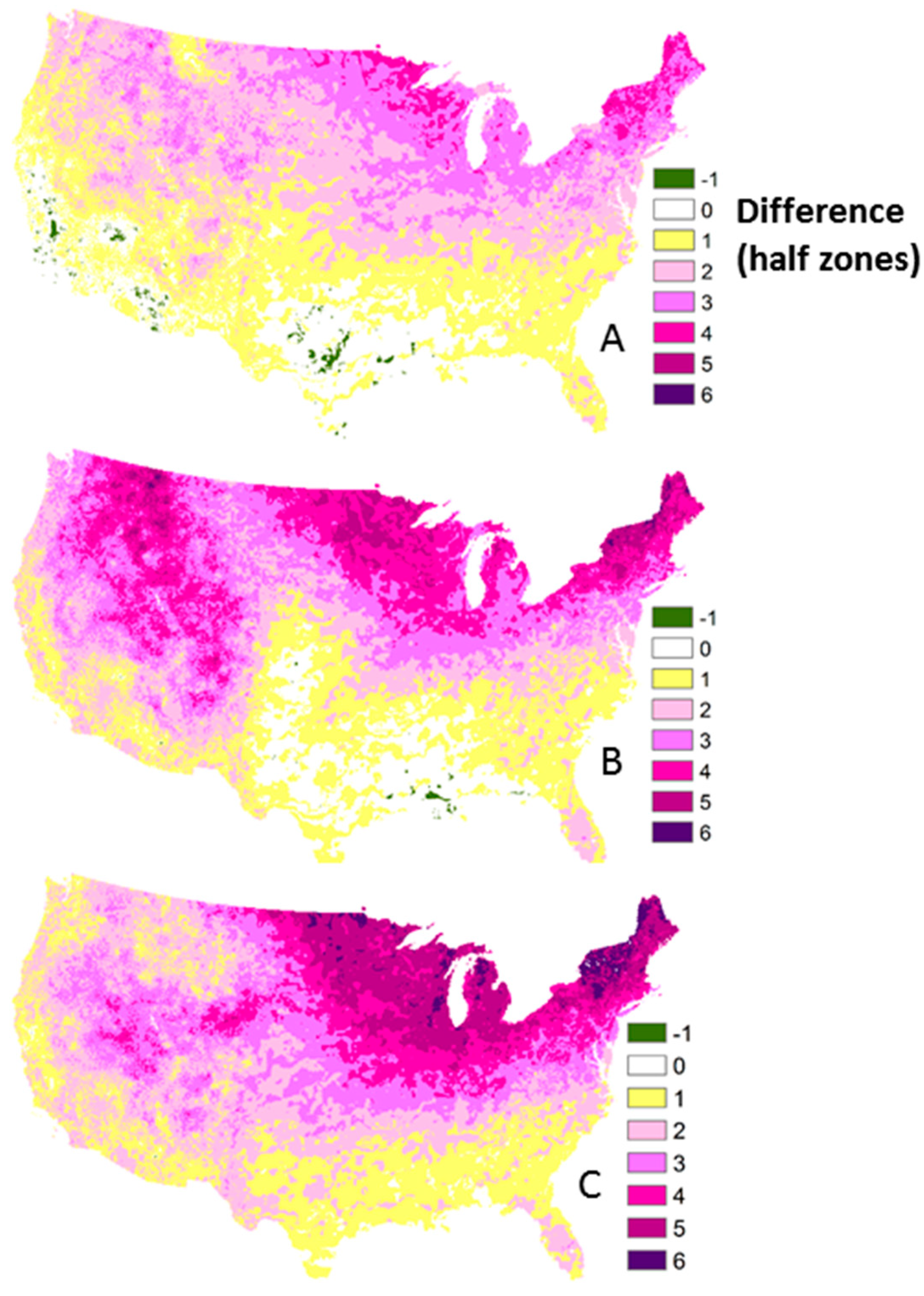
Even though the three projections of future climate varied spatially, as displayed in differences from the current climate in 2.8 °C half zones of plant hardiness zones or coldest days (Figure 1 and Figure 2), the greatest differences from the current climate occurred where temperatures were coldest and the least differences occurred in the southeastern US. The GFDL-ESM2G projected climate was the most balanced, with increasing differences from the current climate northward and slightly eastward. The CanESM2-projected climate had the greatest differences in the mountainous western US and northern states. The HadGEM2-ES-projected climate had the greatest differences in the northeastern quadrant of the US.
Most of the conterminous US currently is in zones 4 to 8, with a mean zone of 6a. Under future climate, most of the conterminous US is projected to be in zones 5 to 9, ranging from a mean of 7a (GFDL-ESM2G) to 7b (CanESM2 and HadGEM2-ES; Supplementary Table S1). Plant hardiness zones ≥7 increased in areal extent and, conversely, plant hardiness zones ≤6 decreased in extent. Under the GFDL-ESM2G projected climate, about 80% of the conterminous US increased by one to three 2.8 °C half zones, while 15% of the area remained within the same plant hardiness zone. Under the CanESM2 projected climate, about 65% of the conterminous US increased by one to three 2.8 °C half zones, 18% of the area increased by four 2.8 °C half zones, while 11% of the area remained within the same plant hardiness zone. Under the HadGEM2-ES projected climate, about 75% of the conterminous US increased by one to three 2.8 °C half zones, 11% of the area increased by four 2.8 °C half zones, 12% of the area increased by five 2.8 °C half zones, while only 1% of the area remained within the same plant hardiness zone.
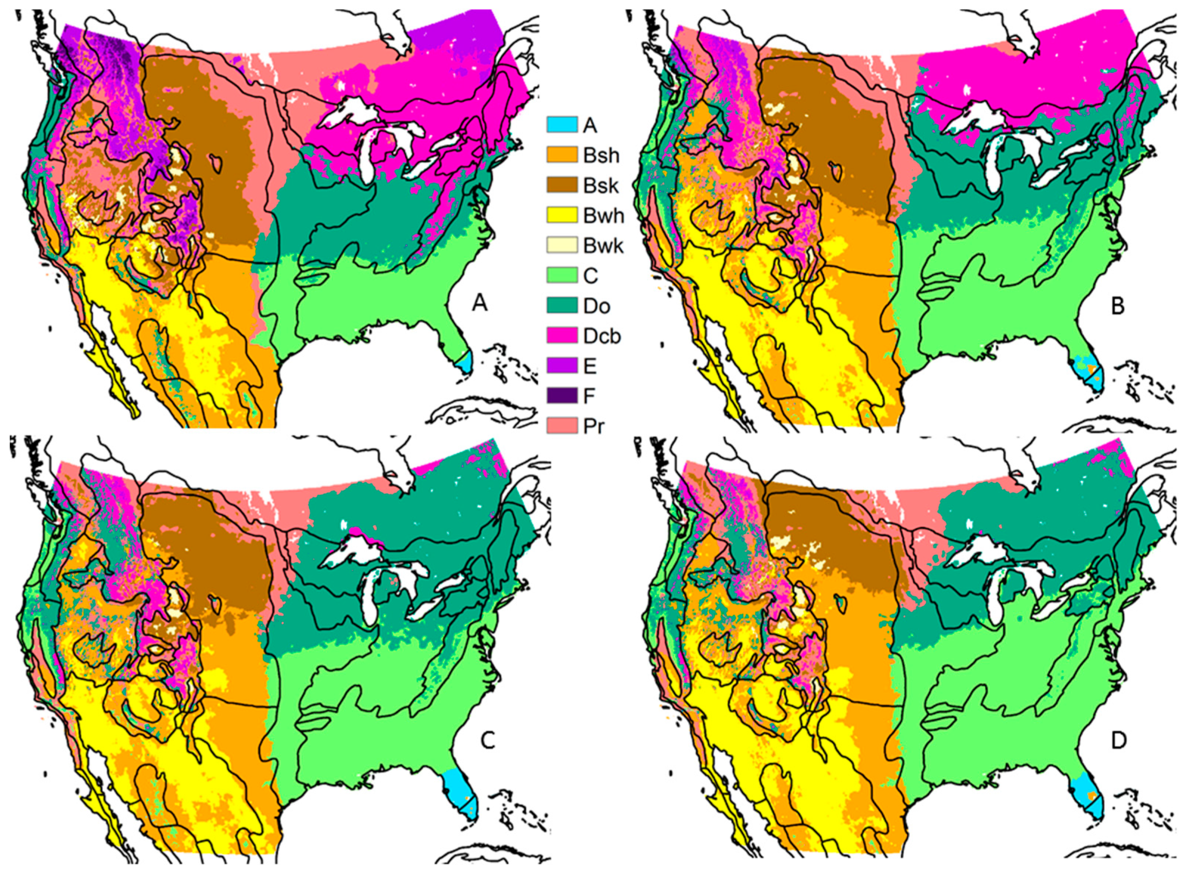
We compared Bailey’s [12] ecological divisions with Köppen-Trewartha’s climate types, which generally overlapped (Figure 3). The extent of the prairie climate type was limited in the central US using these rules and did not match the general outline of the central grassland region [17]. In Bailey’s ecological divisions, the prairie climate type reflects ‘vegetational affinities’ of prairie compared to forest, or a version of the separation of prairie from forest region [17]. We also were not able to differentiate the winter rain and dry summer climates of the West Coast.
The warm continental climate type (Dcb; current area 11% of the conterminous US) shifted out of the eastern US (1% to 4% of area under future climates), and was replaced primarily by the hot continental climate type (Dca; current and future generally about 20% of area, although with a decrease to 15% of the area under HadGEM2-ES; Figure 3, Supplementary Table S2). The subtropical climate type (C; current area 17%) advanced into 50% to 80% of the current hot continental climate type and about 25% of the prairie climate type, expanding to about 30% (GFDL-ESM2G and CanESM2) to 35% (HadGEM2-ES) of the conterminous US. Indeed, under the HadGEM2-ES climate, the subtropical climate type replaced almost 30% of the warm continental climate type. Subtropical steppe (Bsh) expanded from 9% to about 20% of the area and subtropical desert (Bwh) expanded from 5% to about 10% of the area, replacing the temperate steppe (Bsk; 15% of the current area to about 8% of future area). Warmer climate types from both the eastern and western US replaced the prairie climate type (from 17% of the current area to <10% of the future area). Rare, mountainous polar climate types disappeared and boreal climate types contracted in the western mountains (from 4% of the current area to ≤1% of the future area), and the tropical savanna climate type expanded in Florida.
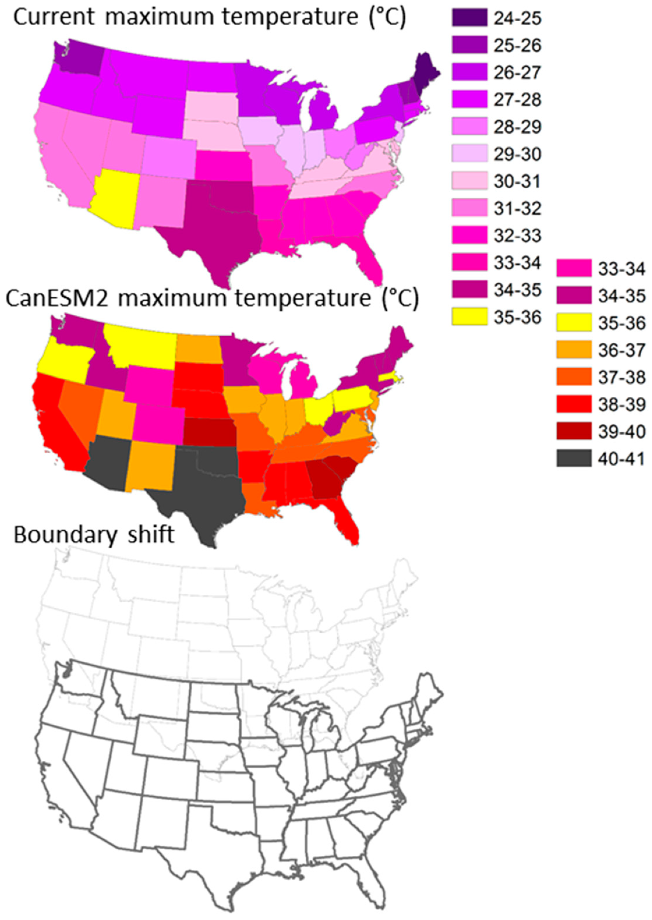
Temperature changes in the hottest months for states averaged 4.9 °C (range 3.5 to 6.7 °C), 6.8 °C (range 4.2 to 9.7 °C), and 8.6 °C (range 5.1 to 12.3 °C) for the GFDL-ESM2G, CanESM2, and HadGEM2-ES climates, respectively. Although state boundaries are stationary, the northernmost tier of states generally may develop the hottest months of the southernmost tier of states under future climates (Figure 4, current climate compared to CanESM2 climate, which expressed a moderate amount of change between GFDL-ESM2G and HadGEM2-ES). That is, Montana’s hottest month in the future became slightly hotter than Arizona’s current hottest month, Wisconsin and Michigan developed the hottest months of Florida and Louisiana, and the hottest months of other northernmost states became at least as hot as the hottest months of Texas and Oklahoma.

4. Discussion

4.1. Ecological Boundary Shifts

The development of GIS has allowed the processing of large spatial datasets to map boundaries related to climate and vegetation. Under future climate, ecological boundaries will move poleward (e.g., Figure 1, Figure 2 and Figure 3), while northern administrative boundaries virtually will become the equivalent of current southern administrative units (e.g., Figure 4). That is, the northern states will acquire the climate of more southern states, and as climate suitability changes, northern terrestrial ecosystems may develop ecological characteristics of more southern ecosystems. Displaying concrete boundary shifts to emphasize potential implications may be more effective than displaying projected increases in temperature, which are seemingly small compared to daily and seasonal temperature variations [18].
Plant survival is closely linked with absolute minimum temperature; hence, the coldest day instead of the hottest day is used to portray climate limitations for plants [19] (Table 1). Plant hardiness zones are a familiar tool and provide tangible connections between climate and appropriate species for the climate [20]. Plant hardiness zones shifted by approximately one (5.6 °C) to one and a half zones (8.4 °C; Figure 1 and Figure 2). Reduced cold hardening, late spring frost damage, and not meeting chilling requirements will potentially affect plant survival and production [20]. Furthermore, warmer extreme minimum temperatures allow expansion of plant pests and pathogens.
Geographic ranges are constrained by where plant species either cannot survive due to freezing or cannot compete well outside of optimum physiological tolerances. Species do not contain genes for or allocate resources to all traits, resulting in a trade-off between cold hardiness and growth rate [21,22]. Seed source or provenance testing of genotypes shows reduced growth rates of northern provenances in warmer locations [23]. Nonetheless, planted trees can survive to maturity hundreds to thousands of kilometers outside of range boundaries [24]. Although there are few studies of physiological tolerances along or outside of range boundaries, established adult trees may not be likely to die immediately, if at all, due to warming climate alone (e.g., without drought; [21]). The temperature range tolerated by established plants may be greater than the range where all life stages can occur, and, thus, a large fraction of the population may persist even where successful reproduction is limited [25,26]. Maintaining growing space will reduce the capture of growing space by more southern species while allowing time to establish and compete against more northern species. Thus, for some plant species, an interval with a climate mismatch may represent lag with relatively few consequences.
Tree species under past warming climate shifted poleward in range [27]. Both statistical and process-based models of tree response to climate typically project an overriding poleward shift as the primary outcome because climate increases of 4 °C to 5 °C in temperature will result in simulated tree movement to suitable climate envelopes (e.g., [28]). Past tree migration in response to climate warming was species-specific [27], and models provide species-specific responses. However, it may be speculative to identify future migration pathways by species, due to many possible factors that may influence species shifts, including species traits, competition, community interactions, disease, continuing disequilibrium since Euro-American settlement, forestry practices, assisted migration by landscape plantings, disruption by urbanization and infrastructure, and other land uses.
Köppen-Trewartha climate types generally shifted into the next poleward ecological region, although subtropical climate types doubled in area by maintaining both current areal extent and capturing area from northern climate types (Figure 3). Even though the climate is warming, at present there is little evidence that North American tree species are shifting latitudinally [29,30]. Given this and historical species-specific migration, it may be unlikely that all species representative of ecological regions will keep pace by moving poleward with climate change or shift in unison. Although some tree species with similar climate restrictions may remain associated with specific Köppen-Trewartha climate types, species characteristic of current ecosystems or associations may not shift with climate at the same rate, direction, or magnitude. In other words, ecosystems or climate types may not maintain the same representation of all tree species, due in part to altered competitive and migration ability under different environmental conditions. If characteristic species shift differentially, mismatches between climate and ecosystems may result.

4.2. Implications

Technical advances in GIS allow visualization of the overall magnitude of potential change for many types of ecosystems under a warming climate. If the northernmost tier of states develops a climate similar to the southernmost tier of states, then northern states may become climatically suitable for southern forests (Figure 4). Moreover, climate classifications (Table 2) approximate the current forest ecosystems. Polar and boreal climate types contracted in western mountains, indicating loss of subalpine or high elevation forests consisting of species such as spruce (Picea) and fir (Abies; Figure 3). Steep elevational gradients that occur at small scales result in both more complex patterning and changes in climate types of the western US than in forests of the eastern US.
The warm continental climate type (Dcb) represents northern mixed forests of the eastern US, generally comprised of distinctive species (i.e., relatively restricted to this region) such as balsam fir (Abies balsamea (L.) Mill.), black and white spruce (Picea mariana (Mill.) Britton, Sterns & Poggenb. and P. glauca (Moench) Voss), jack pine (Pinus banksiana Lamb.), northern white-cedar (Thuja occidentalis L.), paper birch (Betula papyrifera Marsh.), and tamarack (Larix laricina (Du Roi) K. Koch). We note that due to recent forest transitions, red maple (Acer rubrum L.) has become the most abundant species in this region, albeit red maple is competitive under a wide climate range [29]. Red maple is likely to continue increasing because northern mixed forests, as represented by the warm continental climate type, shifted out of the eastern US by 2070 to 2099, replaced primarily by the hot continental climate type (Dca), which approximates eastern broadleaf forests. Eastern broadleaf forests, at least historically, were the center for broadleaf species such as oaks (Quercus), hickories (Carya), and elms (Ulmus). Similarly, the subtropical climate type (C) advanced into the current extent of eastern broadleaf forest and also increased far enough to the north to replace almost 30% of the northern mixed forests or warm continental climate type. The subtropical climate aligns with southeastern mixed forests, which contain characteristic species including longleaf pine (Pinus palustris Mill.) that has become rare, loblolly pine (Pinus taeda L.) and slash pine (Pinus elliottii Engelm.) that have become common as a plantation species, laurel oak (Quercus laurifolia Michx.), sweetgum (Liquidambar styraciflua L.), along with some eastern broadleaf species, such as red maple, that have expanded in recent times [29].
The southern mixed forests also replaced about 25% of the prairie climate type in the Great Plains of the central US to the west of eastern forests (Figure 3, Supplementary Table S2). Trees have been expanding into grasslands for a century or more [31,32] resulting in the loss of the pre-Euro-American settlement boundary line between forests and grasslands [33]. Climate as a barrier between forests and grasslands may be an artificial ecological concept in regions with greater than arid precipitation, and disturbance factors such as fire and grazing may favor grassland vegetation [33,34]. Grassland was not a climate classification type (i.e., no climate ruleset delineates US grasslands, to our knowledge; Table 2) and after attempting different approaches, including evapotranspiration to capture the grasslands, we eventually applied a simple precipitation threshold of 75 cm, approximately a mid-value for grassland biomes. While this classification produced northern grasslands in the central US, which even extended into eastern forests, but not southern grasslands, eastern climate types consisting of forests replaced most of these grasslands under all future climates (Figure 3). However, there is no range of climate too dry for trees in the Great Plains grasslands, as trees exist both in dry, rocky soils of escarpments and in plantations, including mesic species that have survived under the most severe drought periods on record [35].
By the end of the century, ≥85% of the country may be in a different plant hardiness zone (Figure 1 and Figure 2), resulting in mismatches with climate that may be challenging for current plant species, particularly cultivated crops in horticulture and agriculture, including orchards. Plantation trees, which are planted and sometimes grown from genetically improved seedlings, may be more vulnerable to climate change than natural populations. Cultivars are tailored to regional climate and limited genetic diversity of cultivars may result in low adaptive capacity to climate change, particularly increased weather variability and frequency of extreme weather [36].
Although vegetation is more directly related to plant hardiness zones and major ecological regions, there also are ecological consequences for wildlife. Examples include the displacement of wildlife due to loss of habitat (e.g., coldwater fish), food web disruptions due to altered phenology, and heat stress that increases vulnerability to disease and reduces survival and reproduction. Increased precipitation variability and more frequent flooding and drought also affect survival and reproductive success.
Social and economic consequences result from wholesale disruption of climate and ecosystems, such as impacts on agriculture and (agro)forestry, loss of fisheries, reduced food security, reduced water availability, desertification, increased disease, heat stress, flooding, landslides, storm surges, sea level rise, severe wildfires, increased poverty, and increased conflicts. Human civilization developed over the past 10,000 years when temperature and sea levels have been stable [37]. Cities and infrastructure have been built based on current temperatures and sea levels. However, the northernmost tier of US states generally may develop the hottest months of the southernmost tier of states, a shift of 5 °C to 8.6 °C and up to 1500 km, and the sea levels are expected to rise [37]. This creates a host of climate-related spending to adjust infrastructure to new conditions, such as protecting aquifers from exposure to chemicals and saltwater intrusion, increasing water efficiencies to prevent ‘Day Zero’ water crises, and transitioning from heating to cooling of indoor spaces. Every degree Celsius of warming costs about 1.2% of the US gross domestic product [38] and imposes increased social adaptation of living with changes compared to mitigating or limiting changes.

5. Conclusions

Climate change is slow to materialize, and repercussions of the projected temperature change are not readily apparent. Visualization of future changes, using GIS and climate data, allows realization of the magnitude of boundary shifts under future climate change. We applied GIS to demonstrate the magnitude of boundary shifts in plant hardiness zones (i.e., coldest days), Köppen-Trewartha climate types or major ecological regions (combination of minimum and maximum temperatures, precipitation), and the warmest month for US states. The major ecological regions shifted to the extent that both eastern broadleaf forests and southeastern mixed forests replaced northeastern mixed forests in the eastern US. Boundary shifts have ecological, economic, and social ramifications due to undermining established human–environment systems, such as agriculture, forestry, and infrastructure.

Supplementary Materials

The following are available online at https://www.mdpi.com/1999-4907/10/3/280/s1, Table S1: Percent of total area for plant hardiness zones under current climate and GFDL-ESM2G RCP8.5, CanESM2 RCP8.5, and HadGEM2-ES RCP8.5 in the United States, Table S2: Percent of total area for Köppen-Trewartha climate types under current climate and GFDL-ESM2G RCP8.5, CanESM2 RCP8.5, and HadGEM2-ES RCP8.5 in the United States.

Author Contributions

B.B.H. conceived the study and wrote the manuscript. J.S.F. processed data used for analyses and classified and displayed the plant hardiness zones.

Funding

This research received no external funding.

Acknowledgments

We thank anonymous reviewers for their time and careful review.

Conflicts of Interest

The authors declare no conflict of interest.

References

  1. Brysse, K.; Oreskes, N.; O’Reilly, J.; Oppenheimer, M. Climate change prediction: Erring on the side of least drama? Glob. Environ. Chang. 2013, 23, 327–337. [Google Scholar] [CrossRef]
  2. Peters, G.P.; Andrew, R.M.; Boden, T.; Canadell, J.G.; Ciais, P.; Le Quéré, C.; Marland, G.; Raupach, M.R.; Wilson, C. The challenge to keep global warming below 2 °C. Nat. Clim. Chang. 2012, 3, 4–6. [Google Scholar] [CrossRef]
  3. Lazard. Levelized Cost of Energy 2017. Available online: https://www.lazard.com/perspective/levelized-cost-of-energy-2017 (accessed on 1 September 2018).
  4. Kincer, J.B. Atlas of American Agriculture—Climate: Temperature, Sunshine, and Wind; U.S. Government Printing Office: Washington, DC, USA, 1928.
  5. Daly, C.; Widrlechner, M.P.; Halbleib, M.D.; Smith, J.I.; Gibson, W.P. Development of a New USDA Plant Hardiness Zone Map for the United States. J. Appl. Meteorol. Climatol. 2010, 51, 242–264. [Google Scholar] [CrossRef]
  6. Parker, L.E.; Abatzoglou, J.T. Projected changes in cold hardiness zones and suitable overwinter ranges of perennial crops over the United States. Environ. Res. Lett. 2016, 11, 34001. [Google Scholar] [CrossRef] [Green Version]
  7. Köppen, W. ; Volken, E.; Brönnimann, S., Translators; “Die Wärmezonen der Erde, nach der Dauer der heissen, gemässigten und kalten Zeit und nach der Wirkung der Wärme auf die organische Welt betrachtet” [The thermal zones of the earth according to the duration of hot, moderate and cold periods and to the impact of heat on the organic world)]. Meteorol. Zeitschrift 2011, 20, 351–360. [Google Scholar]
  8. Kottek, M.; Grieser, J.; Beck, C.; Rudolf, B.; Rubel, F. World map of the Köppen-Geiger climate classification updated. Meteorol. Zeitschrift 2006, 15, 259–263. [Google Scholar] [CrossRef]
  9. Belda, M.; Holtanová, E.; Halenka, T.; Kalvová, J. Climate classification revisited: From Köppen to Trewartha. Clim. Res. 2014, 59, 1–13. [Google Scholar] [CrossRef]
  10. Ackerman, E.A. The Köppen classification of climates in North America. Geogr. Rev. 1941, 31, 105–111. [Google Scholar] [CrossRef]
  11. Trewartha, G.T. An Introduction to Climate; McGraw-Hill: New York, NY, USA, 1968. [Google Scholar]
  12. Bailey, R.G. Description of the Ecoregions of the United States, 2nd ed.; Misc. Pub. No. 1391; USDA Forest Service: Washington, DC, USA, 1995.
  13. Livneh, B.; Rosenberg, E.A.; Lin, C.; Nijssen, B.; Mishra, V.; Andreadis, K.M.; Maurer, E.P.; Lettenmaier, D.P. A long-term hydrologically based dataset of land surface fluxes and states for the conterminous United States: Update and extensions. J. Clim. 2013, 26, 9384–9392. [Google Scholar] [CrossRef]
  14. Pierce, D.W.; Cayan, D.R.; Thrasher, B.L. Statistical downscaling using Localized Constructed Analogs (LOCA). J. Hydrometeorol. 2014, 15, 2558–2585. [Google Scholar] [CrossRef]
  15. De Castro, M.; Gallardo, C.; Jylha, K.; Tuomenvirta, H. The use of a climate-type classification for assessing climate change effects in Europe from an ensemble of nine regional climate models. Clim. Chang. 2007, 81, 329–341. [Google Scholar] [CrossRef]
  16. Patton, C.P. A note on the classification of dry climate in the Köppen system. Cal. Geogr. 1962, 3, 105–112. [Google Scholar]
  17. Cleland, D.T.; Avers, P.E.; McNab, W.H.; Jensen, M.E.; Bailey, R.G.; King, T.; Russell, W.E. National Hierarchical Framework of Ecological Units. In Ecosystem Management Applications for Sustainable Forest and Wildlife Resources; Boyce, M.S., Haney, A., Eds.; Yale University Press: New Haven, CT, USA, 1997; pp. 181–200. [Google Scholar]
  18. Veloz, S.; Williams, J.W.; Lorenz, D.; Notaro, M.; Vavrus, S.; Vimont, D.J. Identifying climatic analogs for Wisconsin under 21st-century climate-change scenarios. Clim. Chang. 2012, 112, 1037–1058. [Google Scholar] [CrossRef]
  19. Woodward, F.I.; Beerling, D.J. The dynamics of vegetation change: Health warnings for equilibrium “Dodo” models. Glob. Ecol. Biogeogr. Lett. 1997, 6, 413–418. [Google Scholar] [CrossRef]
  20. McKenney, D.W.; Pedlar, J.H.; Lawrence, K.; Papadopol, P.; Campbell, K.; Hutchinson, M.F. Change and evolution in the plant hardiness zones of Canada. Bioscience 2014, 64, 341–350. [Google Scholar] [CrossRef]
  21. Loehle, C. Height growth rate tradeoffs determine northern and southern range limits for trees. J. Biogeogr. 1998, 25, 735–742. [Google Scholar] [CrossRef]
  22. Molina-Montenegro, M.A.; Gallardo-Cerda, J.; Flores, T.S.M.; Atala, C. The trade-off between cold resistance and growth determines the Nothofagus pumilio treeline. Plant Ecol. 2012, 213, 133–142. [Google Scholar] [CrossRef]
  23. Carter, K.K. Provenance tests as Indicators of growth response to climate change in 10 north temperate tree species. Can. J. For. Res. 1996, 26, 1089–1095. [Google Scholar] [CrossRef]
  24. Svenning, J.-C.; Skov, F. Limited filling of the potential range in European tree species. Ecol. Lett. 2004, 7, 565–573. [Google Scholar] [CrossRef]
  25. Pulliam, H.R. Sources, sinks, and population regulation. Am. Nat. 1988, 132, 652–661. [Google Scholar] [CrossRef]
  26. Pulliam, H.R. On the relationship between niche and distribution. Ecol. Lett. 2002, 3, 349–361. [Google Scholar] [CrossRef]
  27. Davis, M.B.; Shaw, R.G. Range shifts and adaptive responses to Quaternary climate change. Science 2001, 292, 673–679. [Google Scholar] [CrossRef]
  28. Iverson, L.R.; Thompson, F.R.; Matthews, S.; Peters, M.; Prasad, A.; Dijak, W.D.; Fraser, J.; Wang, W.J.; Hanberry, B.; He, H.; et al. Multi-model comparison on the effects of climate change on tree species in the eastern U.S.: Results from an enhanced niche model and process-based ecosystem and landscape models. Landsc. Ecol. 2017, 32, 1327–1346. [Google Scholar] [CrossRef]
  29. Hanberry, B.B.; Hansen, M.H. Latitudinal range shifts of tree species in the United States across multi-decadal time scales. Basic Appl. Ecol. 2015, 16, 231–238. [Google Scholar] [CrossRef]
  30. Woodall, C.W.; Westfall, J.A.; D’Amato, A.W.; Foster, J.R.; Walters, B.F. Decadal changes in tree range stability across forests of the eastern U.S. For. Ecol. Manag. 2018, 429, 503–510. [Google Scholar] [CrossRef]
  31. Gleason, H.A. The vegetational history of the Middle West. Ann. Am. Assoc. Geogr. 1922, 12, 39–85. [Google Scholar] [CrossRef]
  32. Hanberry, B.B.; Hansen, M.H. Advancement of tree species across ecotonal borders into non-forested ecosystems. Acta Oecol. 2015, 68, 24–36. [Google Scholar] [CrossRef]
  33. Hanberry, B.B. Defining the historical northeastern forested boundary of the Great Plains grasslands in the United States. Prof. Geogr. in press.
  34. Hanberry, B.B.; Abrams, M.D.; White, J.D. Is increased precipitation during the 20th century statistically or ecologically significant in the eastern US? J. Land Use Sci. 2018, 13, 259–265. [Google Scholar] [CrossRef]
  35. Wells, P.V. Scarp woodlands, transported grassland soils, and concept of grassland climate in the Great Plains region. Science 1965, 148, 246–249. [Google Scholar] [CrossRef]
  36. Hanna, M.; Janne, K.; Perttu, V.; Helena, K. Gaps in the capacity of modern forage crops to adapt to the changing climate in northern Europe. Mitig. Adapt. Strateg. Glob. Chang. 2018, 23, 81–100. [Google Scholar] [CrossRef]
  37. Hansen, J.E.; Sato, M. Paleoclimate implications for human-made climate change. In Climate Change: Inferences from Paleoclimate and Regional Aspects; Berger, A., Mesinger, F., Šijački, D., Eds.; Springer: New York, NY, USA, 2012; pp. 21–48. [Google Scholar]
  38. Hsiang, S.; Kopp, R.; Jina, A.; Rising, J.; Delgado, M.; Mohan, S.; Rasmussen, D.J.; Muir-Wood, R.; Wilson, P.; Oppenheimer, M.; et al. Estimating economic damage from climate change in the United States. Science 2017, 356, 1362–1369. [Google Scholar] [CrossRef] [Green Version]
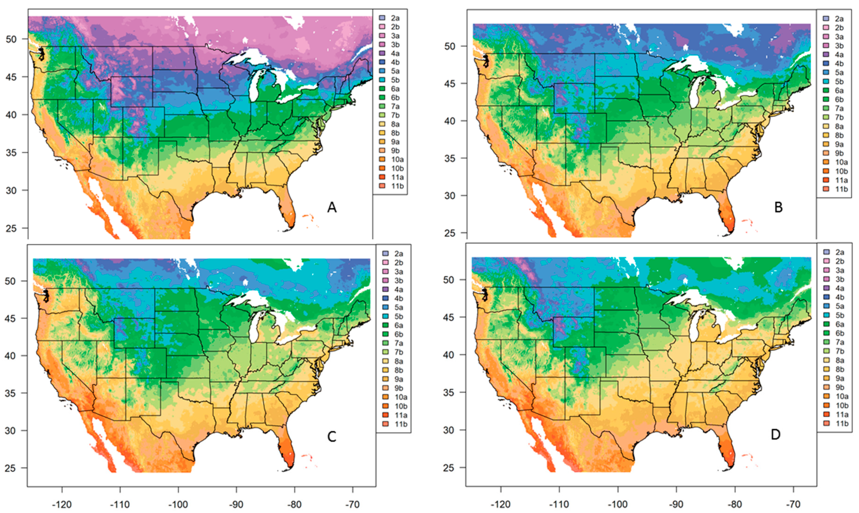
Figure 1. Current plant hardiness zones (panel A) and plant hardiness zones under GFDL-ESM2G RCP8.5 (panel B), CanESM2 RCP8.5 (panel C), and HadGEM2-ES RCP8.5 (panel D).
Forests 10 00280 g001
Figure 2. Differences (future–current plant hardiness zone) between current plant hardiness zones and GFDL-ESM2G RCP8.5 plant hardiness zones (panel A), CanESM2 RCP8.5 plant hardiness zones (panel B), and HadGEM2-ES RCP8.5 plant hardiness zones (panel C).
Forests 10 00280 g002
Figure 3. Current Köppen-Trewartha climate types (panel A) and Köppen-Trewartha climate types under GFDL-ESM2G RCP8.5 (panel B), CanESM2 RCP8.5 (panel C), and HadGEM2-ES RCP8.5 (panel D). For the legend, A = Tropical (Savanna), C = Subtropical and Mediterranean, Dca = Hot Continental, Dcb = Warm Continental, E= Boreal, F = Polar, Bwh = Subtropical desert, Bsh = Subtropical steppe, Bwk = Temperate desert, Bsk = Temperate steppe, Pr = Prairie. Bailey’s [12] ecological divisions are outlined for comparison.
Forests 10 00280 g003
Figure 4. Current hottest month by state and hottest month by state under CanESM2 RCP 8.5.
Forests 10 00280 g004
Table 1. Plant hardiness zones in the United States based on extreme daily minimum temperature during 30 years. Full zones are 5.6 °C (10 °F) and half zones are 2.8 °C (5 °F).
ZoneHalf ZoneMinimum °C (°F)Maximum °C (°F)
2a−45.6 (−50)−42.8 (−45)
b−42.8 (−45)−40 (−40)
3a−40 (−40)−37.2 (−35)
b−37.2 (−35)−34.4 (−30)
4a−34.4 (−30)−31.7 (−25)
b−31.7 (−25)−28.9 (−20)
5a−28.9 (−20)−26.1 (−15)
b−26.1 (−15)−23.3 (−10)
6a−23.3 (−10)−20.6 (−5)
b−20.6 (−5)−17.8 (0)
7a−17.8 (0)−15 (5)
b−15 (5)−12.2 (10)
8a−12.2 (10)−9.4 (15)
b−9.4 (15)−6.7 (20)
9a−6.7 (20)−3.9 (25)
b−3.9 (25)−1.1 (30)
10a−1.1 (30)+1.7 (35)
b1.7 (35)4.4 (40)
11a4.4 (40)7.2 (45)
b7.2 (45)10 (50)
Table 2. Climate types defined by the Köppen-Trewartha climate classification.
Climate TypesLetterRuleset
Tropical (Savanna)Aall months ≥ 18 °C
Subtropical and MediterraneanC8–12 months ≥ 10 °C
Temperate D4–7 months ≥ 10 °C
Hot ContinentalDcawarmest month ≥ 22 °C
Warm ContinentalDcbcoldest month < 0 °C, warmest month < 22 °C
BorealE1 to 3 months ≥ 10 °C
PolarFall months < 10 °C
DryBmean annual precipitation < (2.3 T − 0.64 Pw + 41) a
Subtropical desertBwhmean annual precipitation < 0.5·(2.3 T − 0.64 Pw + 41) a, all months ≥ 0 °C
Subtropical steppeBshmean annual precipitation ≥ 0.5·(2.3 T − 0.64 Pw + 41) a, all months ≥ 0 °C
Temperate desertBwkmean annual precipitation < 0.5·(2.3 T − 0.64 Pw + 41) a, one or more months < 0 °C
Temperate steppeBskmean annual precipitation ≥ 0.5·(2.3 T − 0.64 Pw + 41) a, one or more months < 0 °C
PrairiePrC or D, annual precipitation < 75 cm
a T = mean annual temperature, Pw = % annual precipitation in six winter months.