Forest Growing Stock Volume Estimation in Subtropical Mountain Areas Using PALSAR-2 L-Band PolSAR Data

 , ,
, ,  ,
,  ,
, 
Abstract
1. Introduction
2. Materials
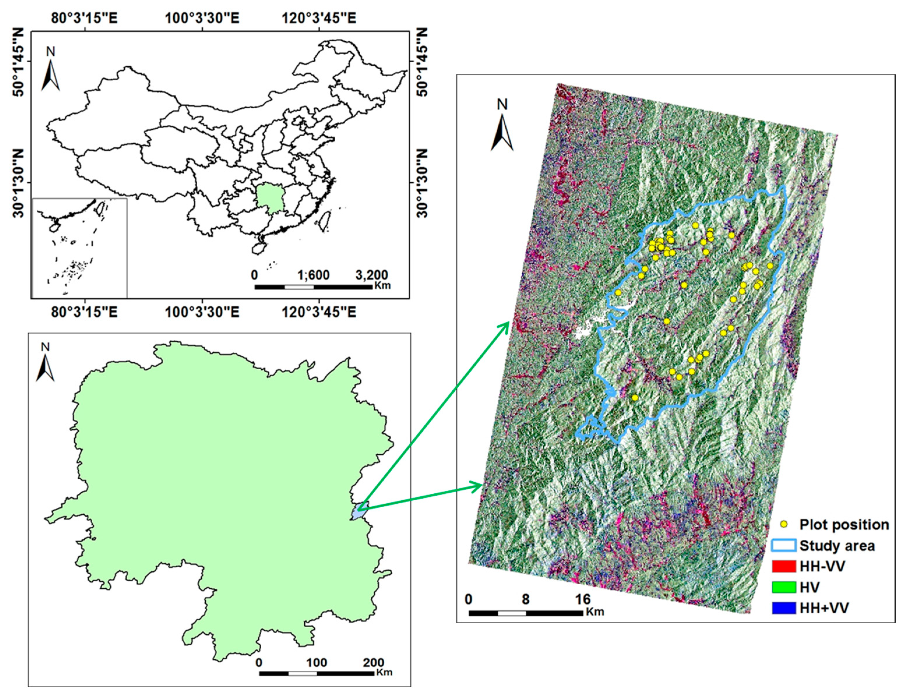
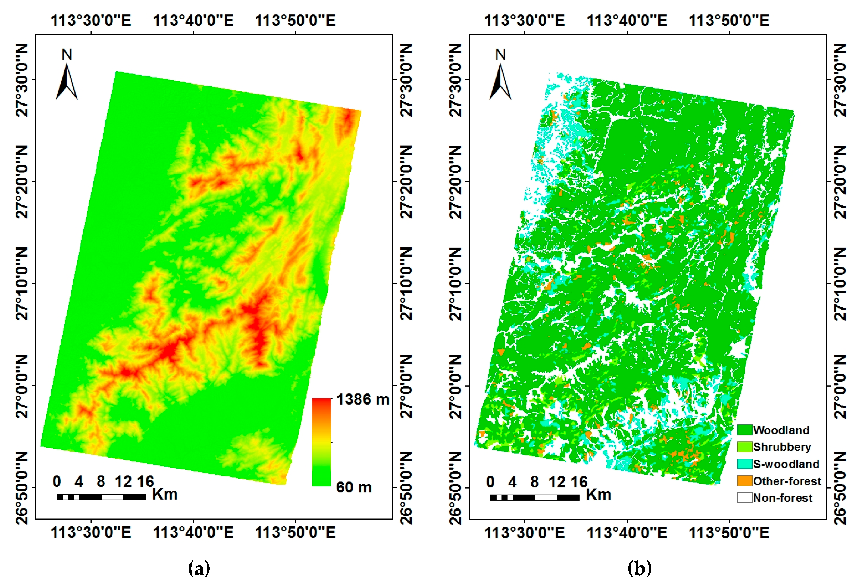
2.1. Study Area
2.2. Field Inventory Data
2.3. Polarimetric SAR Data and Pre-Processing
2.4. Ancillary Data
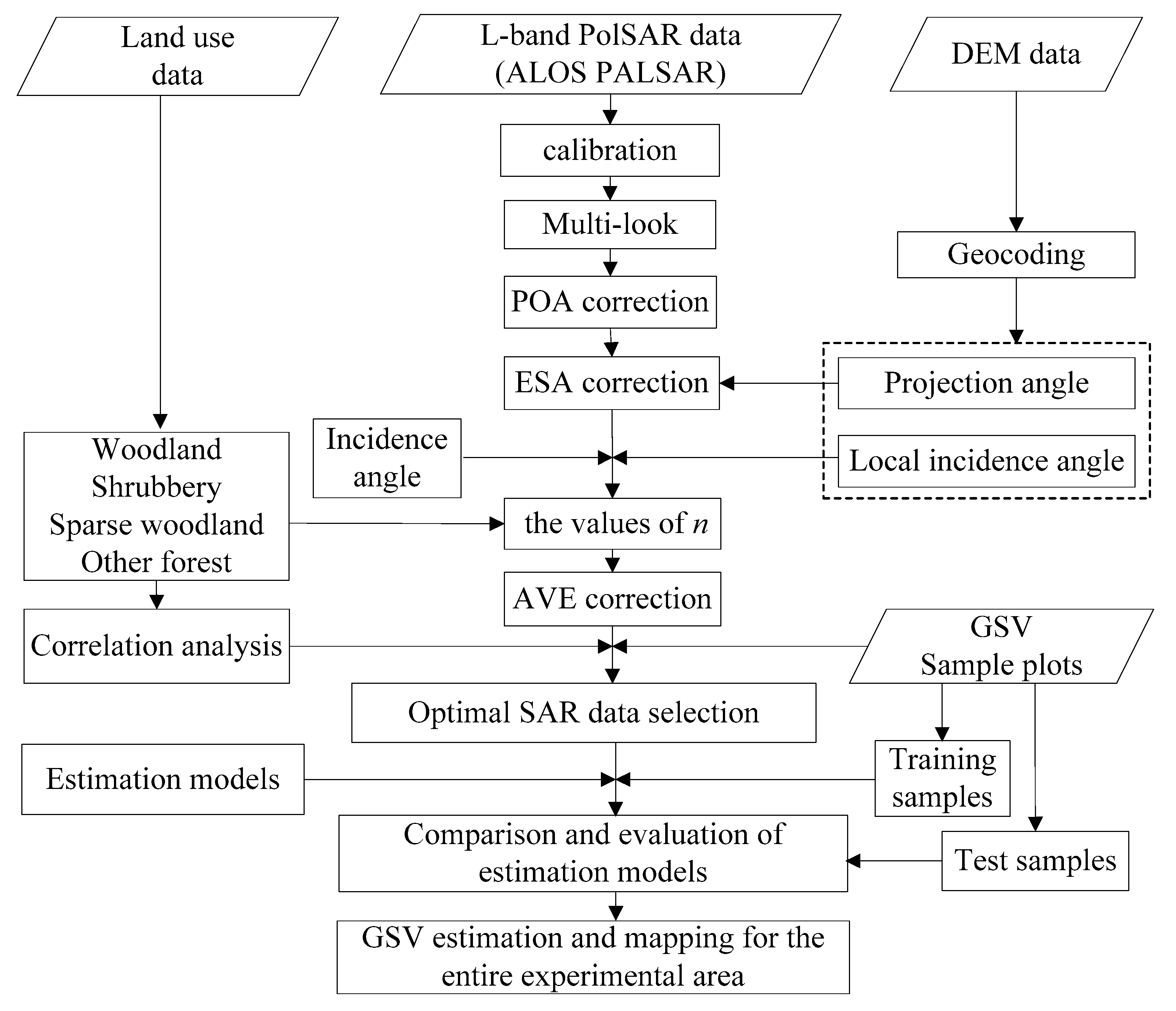
3. Methodology
3.1. Terrain Correction
3.1.1. Polarization Orientation Angle Correction
3.1.2. Effective Scattering Area Correction
3.1.3. Angular Variation Effect Correction
3.2. Retrieval of GSV
4. Results
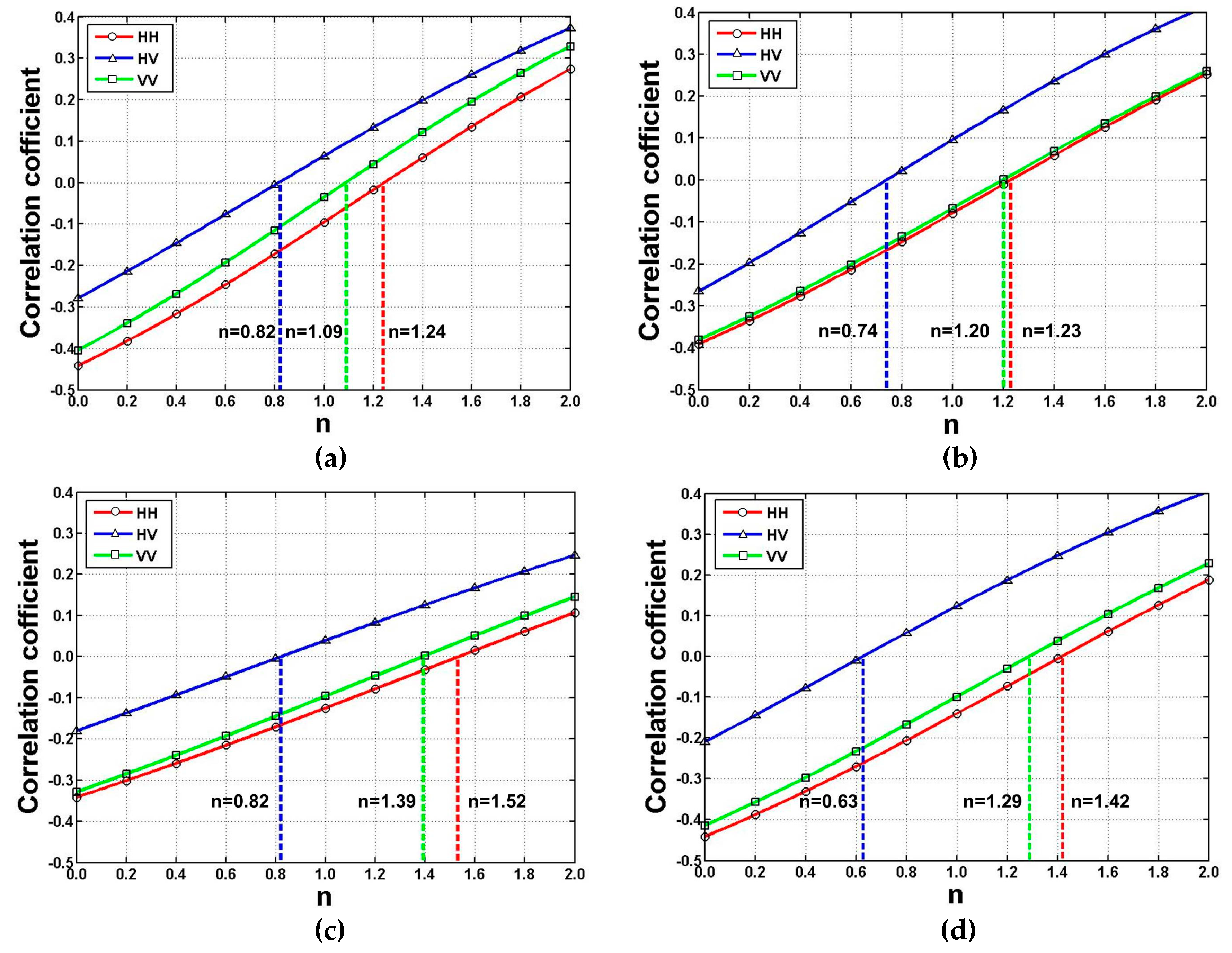
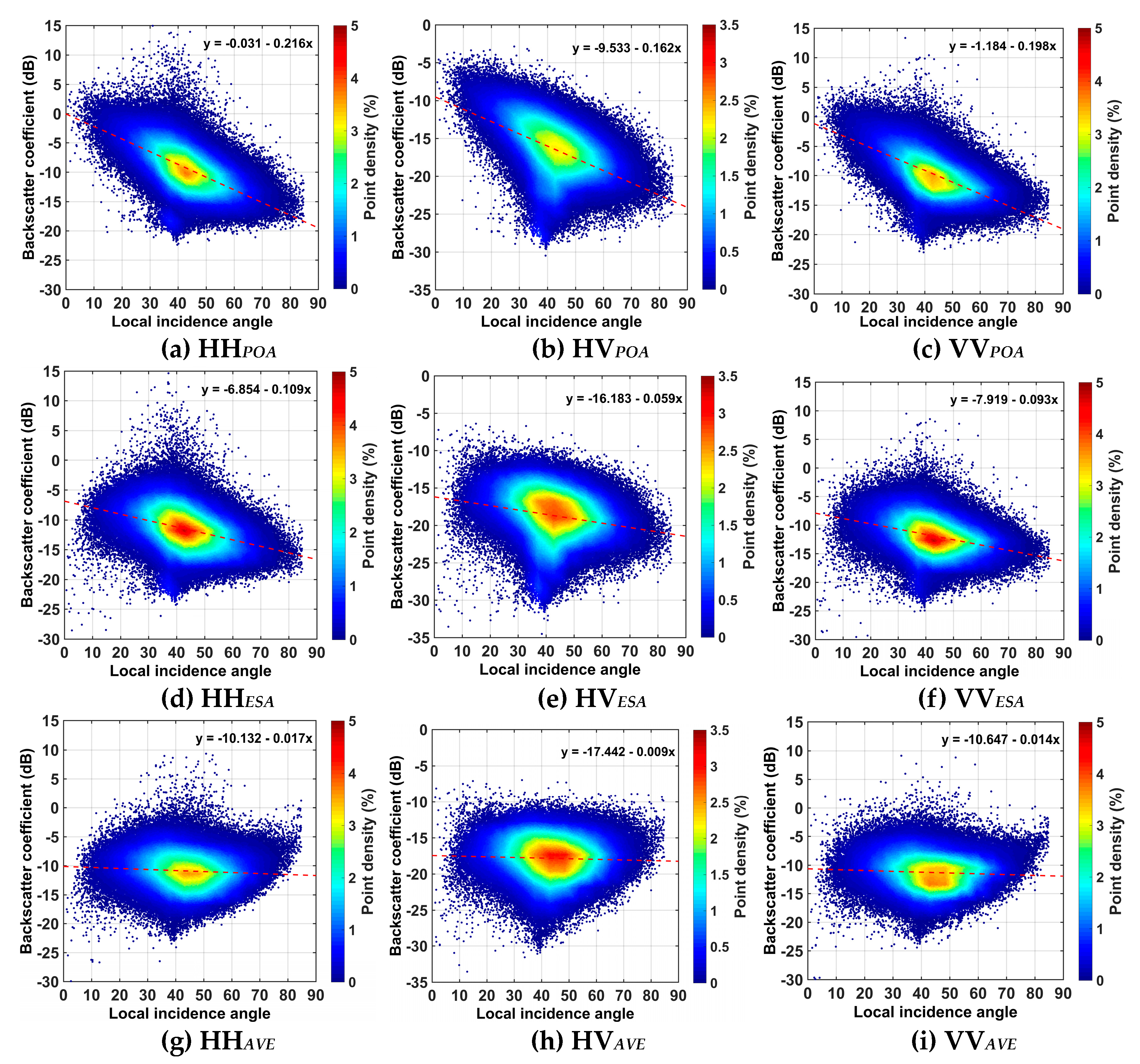
4.1. Acquisition of Terrain Correction Factors
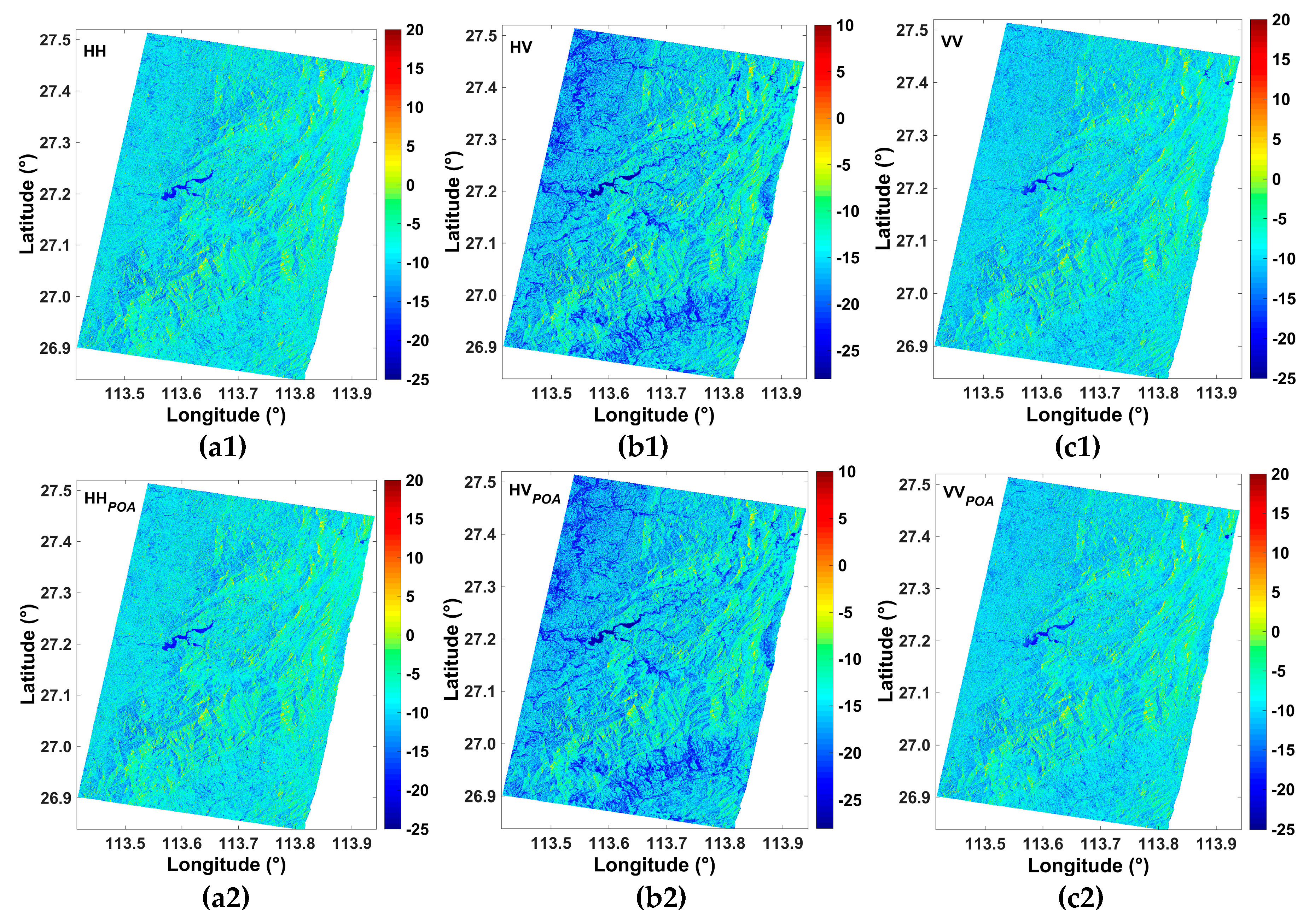
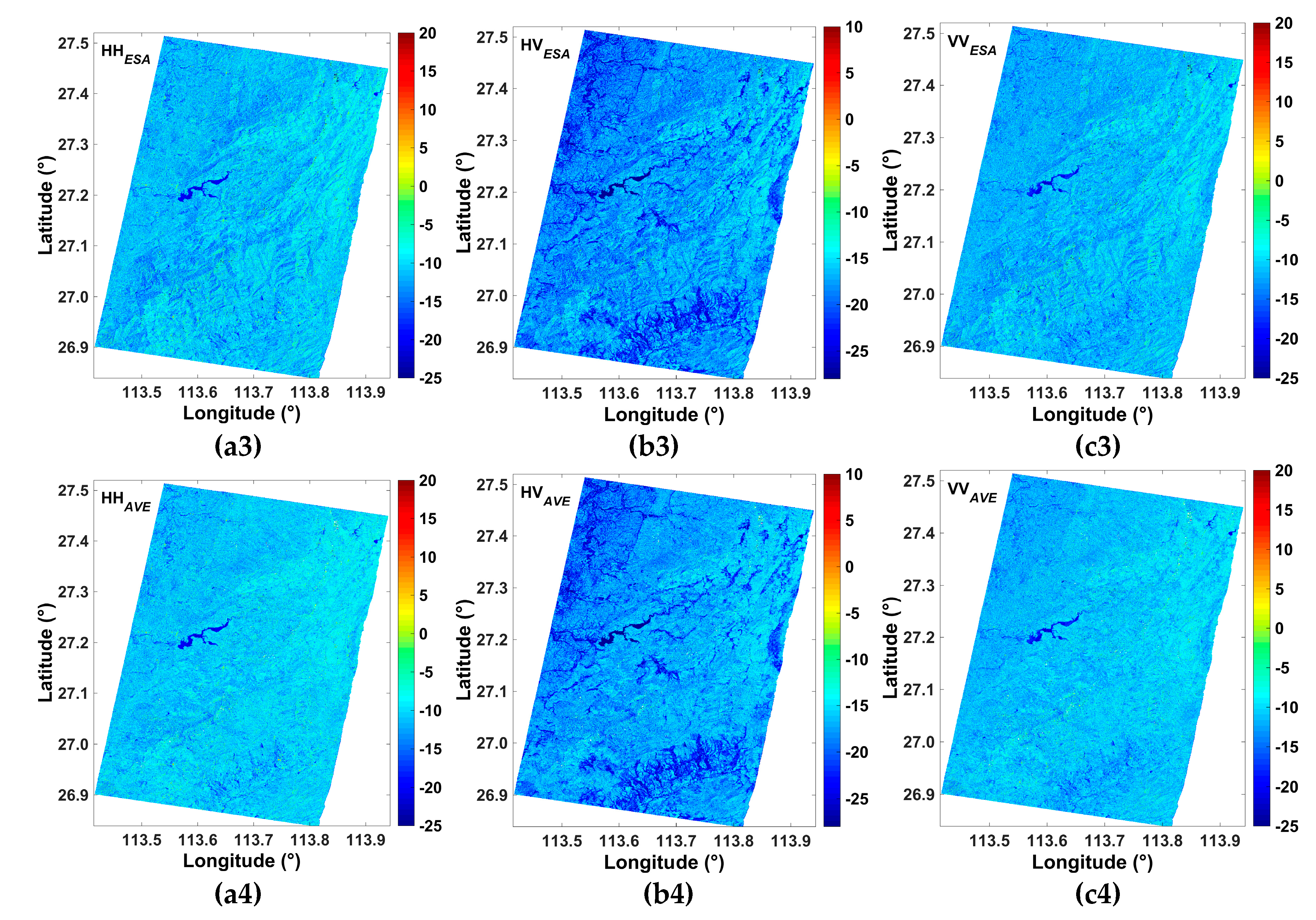
4.2. Results of Terrain Correction
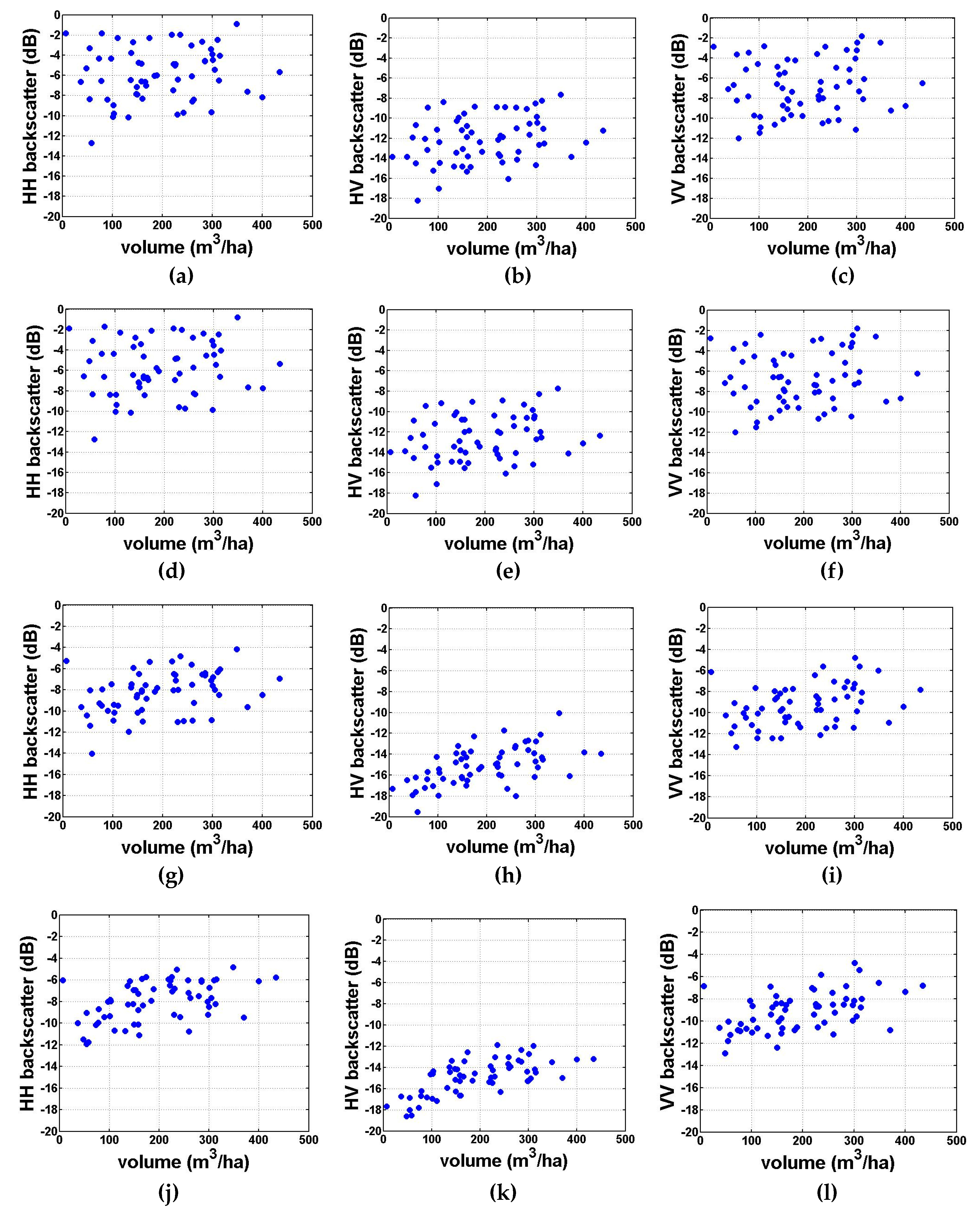
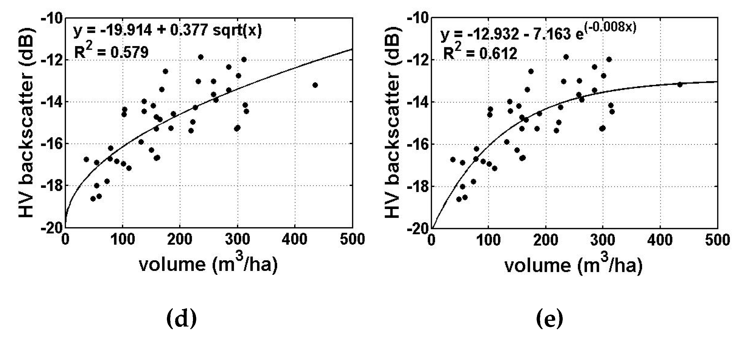
4.3. Backscatter Sensitivity to Forest GSV
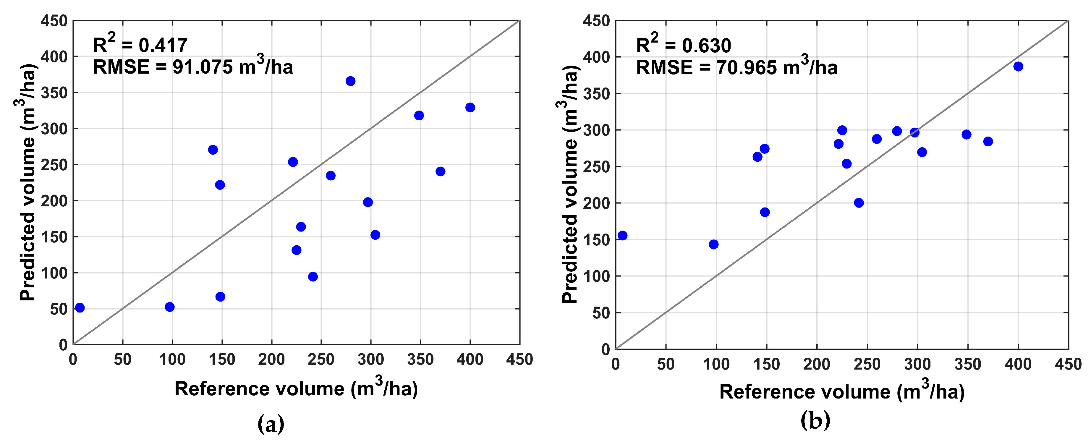
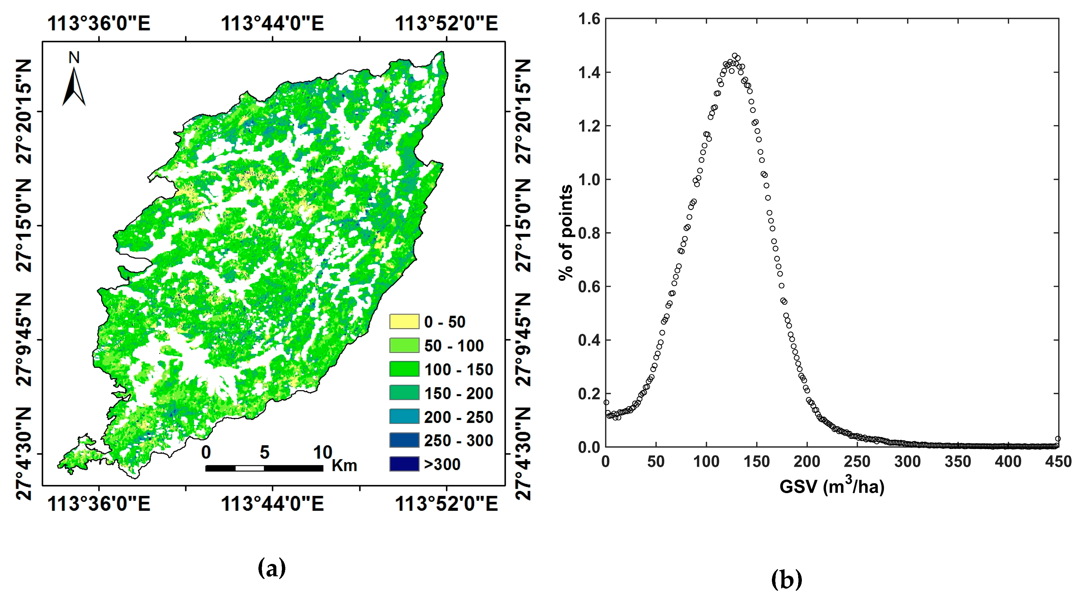
4.4. GSV Estimation and Mapping
5. Discussion
6. Conclusions
Author Contributions
Funding
Acknowledgments
Conflicts of Interest
References
- Houghton, R.A. Aboveground forest biomass and the global carbon balance. Glob. Chang. Biol. 2005, 11, 945–958. [Google Scholar] [CrossRef]
- Shvidenko, A.; Schepaschenko, D.; Nilsson, S.; Bouloui, Y. Semi-empirical models for assessing biological productivity of Northern Eurasian forests. Ecol. Model. 2007, 204, 163–179. [Google Scholar] [CrossRef]
- Santoro, M.; Beaudoin, A.; Beer, C.; Cartus, O.; Fransson, J.E.S.; Hall, R.J.; Pathe, C.; Schmullius, C.; Schepaschenko, D.; Shvidenko, A.; et al. Forest growing stock volume of the northern hemisphere: Spatially explicit estimates for 2010 derived from Envisat ASAR. Remote Sens. Environ. 2015, 168, 316–334. [Google Scholar] [CrossRef]
- Santoro, M.; Cartus, O. Research pathways of forest above-ground biomass estimation based on SAR backscatter and interferometric SAR observations. Remote Sens. 2018, 10, 608. [Google Scholar] [CrossRef]
- Chowdhury, T.A.; Thiel, C.; Schmullius, C. Growing stock volume estimation from L-band ALOS PALSAR polarimetric coherence in Siberian forest. Remote Sens. Environ. 2014, 155, 129–144. [Google Scholar] [CrossRef]
- Song, R.; Lin, H.; Wang, G.; Yan, E.; Ye, Z. Improving selection of spectral variables for vegetation classification of east dongting lake, China, Using a Gaofen-1 image. Remote Sens. 2018, 10, 50. [Google Scholar] [CrossRef]
- Bilous, A.; Myroniuk, A.; Holiaka, D.; Bilous, S.; See, L.; Schepaschenko, D. Mapping growing stock volume and forest live biomass: A case study of the Polissya region of Ukraine. Environ. Res. Lett. 2017, 12, 105001. [Google Scholar] [CrossRef]
- Huete, A.; Didan, K.; Miura, T.; Rodriguez, E.P.; Gao, X.; Ferreira, L.G. Overview of the radiometric and biophysical performance of the MODIS vegetation indices. Remote Sens. Environ. 2002, 83, 195–213. [Google Scholar] [CrossRef]
- Nakaji, T.; Ide, R.; Takagi, K.; Kosugi, Y.; Ohkubo, S.; Nasahara, K.N.; Saigusa, N.; Oguma, H. Utility of spectral vegetation indices for estimation of light conversion efficiency in coniferous forests in Japan. Agric. For. Meteorol. 2008, 148, 776–787. [Google Scholar] [CrossRef]
- Zheng, S.; Gao, C.; Dang, Y.; Xiang, H.; Zhao, J.; Zhang, Y.; Wang, X.; Guo, H. Retrieval of forest growing stock volume by two different methods using Landsat TM images. Int. J. Remote Sens. 2014, 35, 29–43. [Google Scholar] [CrossRef]
- Chrysafis, I.; Mallinis, G.; Siachalou, S.; Patias, P. Assessing the relationships between growing stock volume and sentinel-2 imagery in a Mediterranean forest ecosystem. Remote Sens. Lett. 2017, 8, 508–517. [Google Scholar] [CrossRef]
- Nichol, J.E.; Sarker, M.I.R. Improved biomass estimation using the texture parameters of two high-resolution optical sensors. IEEE Trans. Geosci. Remote Sens. 2011, 49, 930–948. [Google Scholar] [CrossRef]
- Sinha, S.; Jeganathan, C.; Sharma, L.K.; Nathawat, M.S. A review of radar remote sensing for biomass estimation. Int. J. Environ. Sci. Technol. 2015, 12, 1779–1792. [Google Scholar] [CrossRef]
- Donoghue, D.N.M.; Watt, P.J.; Cox, N.J.; Wilson, J. Remote Sensing of Species Mixtures in Conifer Plantations Using LiDAR Height and Intensity Data. Remote Sens. Environ. 2007, 110, 509–522. [Google Scholar] [CrossRef]
- Cartus, O.; Kellndorfer, J.; Rombach, M.; Walker, W. Mapping canopy height and growing stock volume using airborne Lidar, ALOS PALSAR and Landsat ETM+. Remote Sens. 2012, 4, 3320–3345. [Google Scholar] [CrossRef]
- Skowronski, N.S.; Clark, K.L.; Gallagher, M.; Birdsey, R.A.; Hom, J.L. Airborne laser scanner-assisted estimation of aboveground biomass change in a temperate oak-pine forest. Remote Sens. Environ. 2014, 151, 166–174. [Google Scholar] [CrossRef]
- Lu, D.; Chen, Q.; Wang, G.; Li, G.; Moran, E. A survey of remote sensing- based aboveground biomass estimation methods in forest ecosystems. Int. J. Digit. Earth 2014, 9, 63–105. [Google Scholar] [CrossRef]
- Le Toan, T.; Quegan, S.; Davidson, M.W.J.; Balzter, H.; Paillou, P.; Papathanassiou, K.; Plummer, S.; Rocca, F.; Saatchi, S.; Shugart, H.; et al. The BIOMASS Mission: Mapping global forest biomass to better understand the terrestrial carbon cycle. Remote Sens. Environ. 2011, 115, 2850–2860. [Google Scholar] [CrossRef]
- Fu, H.; Zhu, J.; Wang, C.; Wang, H.; Zhao, R. Underlying topography estimation over forest areas using high-resolution P-band Single-baseline PolInSAR data. Remote Sens. 2017, 9, 363. [Google Scholar] [CrossRef]
- Wang, C.; Cai, J.; Li, Z.; Mao, X.; Feng, G.; Wang, Q. Kinematic parameter inversion of the slumgullion landslide using the time series offset tracking method with UAVSAR data. J. Geophys Res. Solid Earth 2018, 10, 1029. [Google Scholar] [CrossRef]
- Xie, Q.; Zhu, J.; Lopez-Sanchez, J.M.; Wang, C.; Fu, H. A modified general polarimetric model-based decomposition method with the simplified Neumann volume scattering model. IEEE Geosci. Remote Sens. Lett. 2018, 15, 1229–1233. [Google Scholar] [CrossRef]
- Gao, H.; Wang, C.; Wang, G.; Zhu, J.; Tang, Y.; Shen, P.; Zhu, Z. A crop classification method integrating GF-3 PolSAR and Sentinel-2A optical data in the Dongting Lake Basin. Sensors 2018, 18, 3139. [Google Scholar] [CrossRef]
- Sandberg, G.; Ulander, L.M.H.; Fransson, J.E.S.; Holmgren, J.; Le Toan, T. L-and P-band backscatter intensity for biomass retrieval in hemiboreal forest. Remote Sens. Environ. 2011, 115, 2874–2886. [Google Scholar] [CrossRef]
- Mermoz, S.; Réjou-Méchain, M.; Villard, L.; Le Toan, T.; Rossi, V.; Gourlet-Fleury, S. Decrease of L-band SAR backscatter with biomass of dense forests. Remote Sens. Environ. 2015, 159, 307–317. [Google Scholar] [CrossRef]
- Wu, C.; Wang, C.; Shen, P.; Zhu, J.; Fu, H.; Gao, H. Forest height estimation using PolInSAR optimal normal matrix constraint and cross-iteration method. IEEE Geosci. Remote Sens. Lett. 2019. [Google Scholar] [CrossRef]
- Ma, J.; Xiao, X.; Qin, Y.; Chen, B.; Hu, Y.; Li, X.; Zhao, B. Estimating aboveground biomass of broadleaf, needleleaf, and mixed forests in Northeastern China through analysis of 25-m ALOS/PALSAR mosaic data. For. Ecol. Manag. 2017, 389, 199–210. [Google Scholar] [CrossRef]
- Treuhaft, R.N.; Goncalves, F.G.; Drake, J.B.; Chapman, B.D.; Santos, J.R.D.; Dutra, L.V.; Graca, P.M.L.A.; Purcell, G.H. Biomass estimation in a Tropical Wet forest using Fourier transforms of profiles from lidar or interferometric SAR. Geophys Res. Lett. 2010, 37, 225. [Google Scholar] [CrossRef]
- Thiel, C.; Schmullius, C. The potential of ALOS PALSAR backscatter and InSAR coherence for forest growing stock volume estimation in Central Siberia. Remote Sens. Environ. 2016, 173, 258–273. [Google Scholar] [CrossRef]
- Tebaldini, S. Algebraic synthesis of forest scenarios from multibaseline PolInSAR data. IEEE Trans. Geosci. Remote Sens. 2009, 47, 4132–4144. [Google Scholar] [CrossRef]
- Cloude, S.R. Polarization coherence tomography. Radio Sci. 2006, 41, RS4017. [Google Scholar] [CrossRef]
- Li, W.; Chen, E.; Li, Z.; Ke, Y.; Zhan, W. Forest aboveground biomass estimation using polarization coherence tomography and PolSAR segmentation. Int. J. Remote Sens. 2015, 36, 530–550. [Google Scholar] [CrossRef]
- Zhang, H.; Wang, C.; Zhu, J.; Fu, H.; Xie, Q.; Shen, P. Forest above-ground biomass estimation using single-baseline polarization coherence tomography with P-band PolInSAR data. Forests 2018, 9, 163. [Google Scholar] [CrossRef]
- Minh, D.H.T.; Le Toan, T.; Rocca, F.; Tebaldini, S.; Villard, L.; Réjou-Méchain, M.; Phillips, O.L.; Feldpausch, T.R.; Dubois-Fernandez, P.; Scipal, K.; et al. SAR tomography for the retrieval of forest biomass and height: Cross-validation at two tropical forest sites in French Guiana. Remote Sens. Environ. 2016, 175, 138–147. [Google Scholar] [CrossRef]
- Peng, X.; Li, X.; Wang, C.; Fu, H.; Du, Y. A maximum likelihood based nonparametric iterative adaptive radar tomography and its application for estimating underlying topography and forest height. Sensors 2018, 18, 2459. [Google Scholar] [CrossRef]
- Peng, X.; Wang, C.; Li, X.; Du, Y.; Fu, H.; Yang, Z.; Xie, Q. Three-Dimensional structure inversion of buildings with nonparametric iterative adaptive approach using SAR tomography. Remote Sens. 2018, 10, 1004. [Google Scholar] [CrossRef]
- Lee, J.S.; Pottier, E. Polarimetric Radar Imaging: From Basics to Applications; CRC Press, Taylor & Francis Group: Boca Raton, FL, USA, 2009. [Google Scholar]
- Chowdhury, T.A.; Thiel, C.; Schmullius, C.; Stelmaszczukgórska, M. Polarimetric parameters for growing stock volume estimation using ALOS PALSAR L-band data over Siberian forests. Remote Sens. 2013, 5, 5725–5726. [Google Scholar] [CrossRef]
- Le Toan, T.; Quegan, S.; Woodward, I.; Lomas, M.; Delbart, N.; Picard, C. Relationg radar remote sensing of biomass to modeling of forest carbon budgets. Clim. Chang. 2004, 76, 379–402. [Google Scholar] [CrossRef]
- Lucas, R.; Armston, J.; Fairfax, R.; Fensham, R.; Accad, A.; Carreiras, J.; Kelley, J.; Bunting, P.; Clewley, D.; Bray, S.; et al. An evaluation of the ALOS PALSAR L-band backscatter-Above ground biomass relationship Queensland, Australia: Impacts of surface moistrure condition and vegetation structure. IEEE J. Sel. Top. Appl. Earth Obs. Remote Sens. 2010, 3, 576–593. [Google Scholar] [CrossRef]
- Wilhelm, S.; Hüttich, C.; Korets, M.; Schmullius, C. Large area mapping of boreal growing stock volume on an annual and multi-temporal level using PALSAR L-band backscatter mosaics. Forests 2014, 5, 1999–2015. [Google Scholar] [CrossRef]
- Mermoz, S.; Le Toan, T.; Villard, L.; Réjou-méchain, M.; Seifert-Granzin, J. Biomass assessment in the Cameroon savanna using ALOS PALSAR data. Remote Sens. Environ. 2014, 155, 109–119. [Google Scholar] [CrossRef]
- Urbazaev, M.; Thiel, C.; Mathieu, R.; Naidoo, L.; Levick, S.R.; Smit, I.P.J.; Asner, G.P.; Schmullius, C. Assessment of the mapping of fractional woody cover in southern African savannas using multi-temporal and polarimetric ALOS PALSAR L-band images. Remote Sens. Environ. 2015, 166, 138–153. [Google Scholar] [CrossRef]
- Antropov, O.; Rauste, Y.; Häme, T.; Praks, J. Polarimetric ALOS PALSAR time series in mapping biomass of boreal forests. Remote Sens. 2017, 9, 999. [Google Scholar] [CrossRef]
- Zhao, P.P.; Lu, D.S.; Wang, G.X.; Liu, L.J.; Li, D.Q.; Zhu, J.R.; Yu, S.Q. Forest aboveground biomass estimation in Zhejiang province using the integration of Landsat TM and ALOS PALSAR data. Int. J. Appl. Earth Obs. 2016, 53, 1–15. [Google Scholar] [CrossRef]
- Bouvet, A.; Mermoz, S.; Le Toan, T.; Villard, L.; Mathieu, R.; Naidoo, L.; Asner, G.P. An above-ground biomass map of African savannahs and woodlands at 25m resolution derived from ALOS PALSAR. Remote Sens. Environ. 2018, 206, 156–173. [Google Scholar] [CrossRef]
- Ningthoujam, R.K.; Joshi, P.K.; Roy, P.S. Retrieval of forest biomass for tropical deciduous mixed forest using ALOS PALSAR mosaic imagery and field plot data. Int. J. Appl. Earth Obs. Geoinform. 2018, 69, 206–216. [Google Scholar] [CrossRef]
- Lee, J.S.; Ainsworth, T.L. The effect of orientation angle compensation on coherency matrix and polarimetric target decomposition. IEEE Trans. Geosci. Remote Sens. 2011, 49, 53–64. [Google Scholar] [CrossRef]
- Small, D. Flattening gamma: Radiometric terrain correction for SAR imagery. TEEE Trans. Geosci. Remote Sens. 2011, 49, 3081–3093. [Google Scholar] [CrossRef]
- Castel, T.; Beaudoin, A.; Stach, N.; Le Toan, T.; Durand, P. Sensitivity of space-borne SAR data to forest parameters over sloping terrain. Theory and experiment. Int. J. Remote Sens. 2001, 22, 2351–2376. [Google Scholar] [CrossRef]
- Zhao, L.; Chen, E.; Li, Z.; Zhang, W.; Gu, X. Three-step semi-empirical radiometric terrain correction approach for PloSAR data applied to forested areas. Remote Sens. 2017, 9, 269. [Google Scholar] [CrossRef]
- Deng, S.; Katoh, M.; Guan, Q.; Yin, N.; Li, M. Estimating forest aboveground biomass by combining ALOS PALSAR and WorldView-2 data: A case study at purple mountain national park, Nanjing, China. Remote Sens. 2014, 6, 7878–7910. [Google Scholar] [CrossRef]
- Fang, J.; Liu, G.; Xu, S. Biomass and net production of forest vegetation in China. Acta Ecol. Sin. 1996, 16, 497–508. [Google Scholar]
- Shimada, M.; Isoguchi, O.; Tadono, T.; Isono, K. PALSAR radiometric and geometric calibration. IEEE Trans. Geosci. Reomte Sens. 2009, 47, 3915–3932. [Google Scholar] [CrossRef]
- Lee, J.S.; Schuler, D.L.; Ainsworth, T.L. Polarimetric SAR data compensation for terrain azimuth slope variation. IEEE Trans. Geosci. Remote Sens. 2000, 38, 2153–2163. [Google Scholar]
- Ulander, L.M.H. Radiometric slope correcton of synthetic-aperture radar images. IEEE Trans. Geosci. Rmote Sens. 1996, 34, 1115–1122. [Google Scholar] [CrossRef]
- Ulaby, F.T.; Moore, R.K.; Fung, A.K. Volume Scattering and Emission Theory. In Microwave Remote Sensing Active and Passive; Artech House: Norwood, MA, USA, 1982; Volume III. [Google Scholar]
- Peregon, A.; Yamagata, Y. The use of ALOS/PALSAR backscatter to estimation above-ground forest biomass: A case study in Western Siberia. Remote Sens. Environ. 2013, 137, 139–146. [Google Scholar] [CrossRef]
- Pham, T.D.; Yoshino, K. Aboveground biomass estimation of mangrove species using ALOS-2 PALSAR imagery in Hai Phong city, Vietnam. J. Appl. Remote Sens. 2017, 11, 026010. [Google Scholar] [CrossRef]
- Villard, L.; Le Toan, T. Relating P-band SAR intensity to biomass for tropical dense forests in Hilly terrain: γ0 or t0. IEEE J. Sel. Top. Appl. Earth Obs. Remote Sens. 2015, 8, 214–223. [Google Scholar] [CrossRef]
- Cartus, O.; Santoro, M.; Kellndorfer, J. Mapping forest aboveground biomass in the Northeastern United States with ALOS PALSAR dual-polarization L-band. Remote Sens. Environ. 2012, 124, 466–478. [Google Scholar] [CrossRef]
- Attarchi, S.; Gloaguen, R. Improving the estimation of above ground biomass using dual polarimetric PALSAR and ETM+ data in the Hyrcanian Mountain forest (Iran). Remote Sens. 2014, 6, 3693–3715. [Google Scholar] [CrossRef]
- Thiel, C.J.; Thiel, C.; Schmullius, C.C. Operational large-area forest monitoring in Siveria using ALOS PALSAR summer intensities and winter coherence. IEEE Trans. Geosci. Remote Sens. 2009, 47, 3993–4000. [Google Scholar] [CrossRef]
- Kim, C. Quantataive analysis of relationship between ALOS PALSAR backscatter and forest stand volume. J. Mar. Sci. Technol. 2012, 20, 624–628. [Google Scholar]


| Range | Mean | |
|---|---|---|
| DBH | 4.06 to 30.10 cm | 17.84 cm |
| Height | 4.60 to 20.20 m | 13.24 m |
| Number of Stems | 30 to 350 | 96 |
| Growing Stock Volume | 6.88 to 434.42 m3/ha | 194.75 m3/ha |
| Data | Woodland | Shrubbery | S-Woodland | O-Forest | |
|---|---|---|---|---|---|
| HH | 16 June 2016 | 1.31 | 1.27 | 1.60 | 1.48 |
| 30 June 2016 | 1.20 | 1.41 | 1.50 | 1.37 | |
| 14 July 2016 | 1.24 | 1.23 | 1.52 | 1.42 | |
| 11 August 2016 | 1.11 | 1.09 | 1.30 | 1.22 | |
| 25 August 2016 | 1.13 | 1.06 | 1.36 | 1.25 | |
| 22 September 2016 | 1.16 | 1.12 | 1.37 | 1.24 | |
| 6 October 2016 | 1.32 | 1.35 | 1.58 | 1.46 | |
| HV | 16 June 2016 | 0.91 | 0.83 | 0.93 | 0.77 |
| 30 June 2016 | 0.76 | 0.67 | 0.79 | 0.57 | |
| 14 July 2016 | 0.82 | 0.74 | 0.82 | 0.63 | |
| 11 August 2016 | 0.74 | 0.65 | 0.65 | 0.48 | |
| 25 August 2016 | 0.74 | 0.63 | 0.67 | 0.47 | |
| 22 September 2016 | 0.70 | 0.56 | 0.65 | 0.44 | |
| 6 October 2016 | 0.85 | 0.79 | 0.83 | 0.64 | |
| VV | 16 June 2016 | 1.14 | 1.24 | 1.44 | 1.38 |
| 30 June 2016 | 1.04 | 1.14 | 1.36 | 1.26 | |
| 14 July 2016 | 1.09 | 1.20 | 1.39 | 1.29 | |
| 11 August 2016 | 1.01 | 1.11 | 1.20 | 1.14 | |
| 25 August 2016 | 1.01 | 1.06 | 1.22 | 1.11 | |
| 22 September 2016 | 1.01 | 1.10 | 1.23 | 1.13 | |
| 6 October 2016 | 1.13 | 1.29 | 1.42 | 1.34 |
| Acquisition Time | HH | HV | VV |
|---|---|---|---|
| 16 June 2016 | 0.418 | 0.495 | 0.370 |
| 30 June 2016 | 0374 | 0.561 | 0.216 |
| 14 July 2016 | 0.489 | 0.643 | 0.473 |
| 11 August 2016 | 0.435 | 0.564 | 0.377 |
| 25 August 2016 | 0.469 | 0.563 | 0.428 |
| 22 September 2016 | 0.182 | 0.545 | 0.123 |
| 6 October 2016 | 0.381 | 0.487 | 0.349 |
| Model | Regression Equation | R2 |
|---|---|---|
| Direct linear | 0.529 | |
| Logarithmic | 0.601 | |
| Quadratic | 0.603 | |
| Exponential | 0.579 | |
| Water-Cloud analysis | 0.612 | |
| Multi-variable | 0.674 |
© 2019 by the authors. Licensee MDPI, Basel, Switzerland. This article is an open access article distributed under the terms and conditions of the Creative Commons Attribution (CC BY) license (http://creativecommons.org/licenses/by/4.0/).
Share and Cite
Zhang, H.; Zhu, J.; Wang, C.; Lin, H.; Long, J.; Zhao, L.; Fu, H.; Liu, Z. Forest Growing Stock Volume Estimation in Subtropical Mountain Areas Using PALSAR-2 L-Band PolSAR Data. Forests 2019, 10, 276. https://doi.org/10.3390/f10030276
Zhang H, Zhu J, Wang C, Lin H, Long J, Zhao L, Fu H, Liu Z. Forest Growing Stock Volume Estimation in Subtropical Mountain Areas Using PALSAR-2 L-Band PolSAR Data. Forests. 2019; 10(3):276. https://doi.org/10.3390/f10030276
Chicago/Turabian StyleZhang, Haibo, Jianjun Zhu, Changcheng Wang, Hui Lin, Jiangping Long, Lei Zhao, Haiqiang Fu, and Zhiwei Liu. 2019. "Forest Growing Stock Volume Estimation in Subtropical Mountain Areas Using PALSAR-2 L-Band PolSAR Data" Forests 10, no. 3: 276. https://doi.org/10.3390/f10030276
APA StyleZhang, H., Zhu, J., Wang, C., Lin, H., Long, J., Zhao, L., Fu, H., & Liu, Z. (2019). Forest Growing Stock Volume Estimation in Subtropical Mountain Areas Using PALSAR-2 L-Band PolSAR Data. Forests, 10(3), 276. https://doi.org/10.3390/f10030276