Low Divergence Among Natural Populations of Cornus kousa subsp. chinensis Revealed by ISSR Markers


Abstract
1. Introduction
2. Materials and Methods
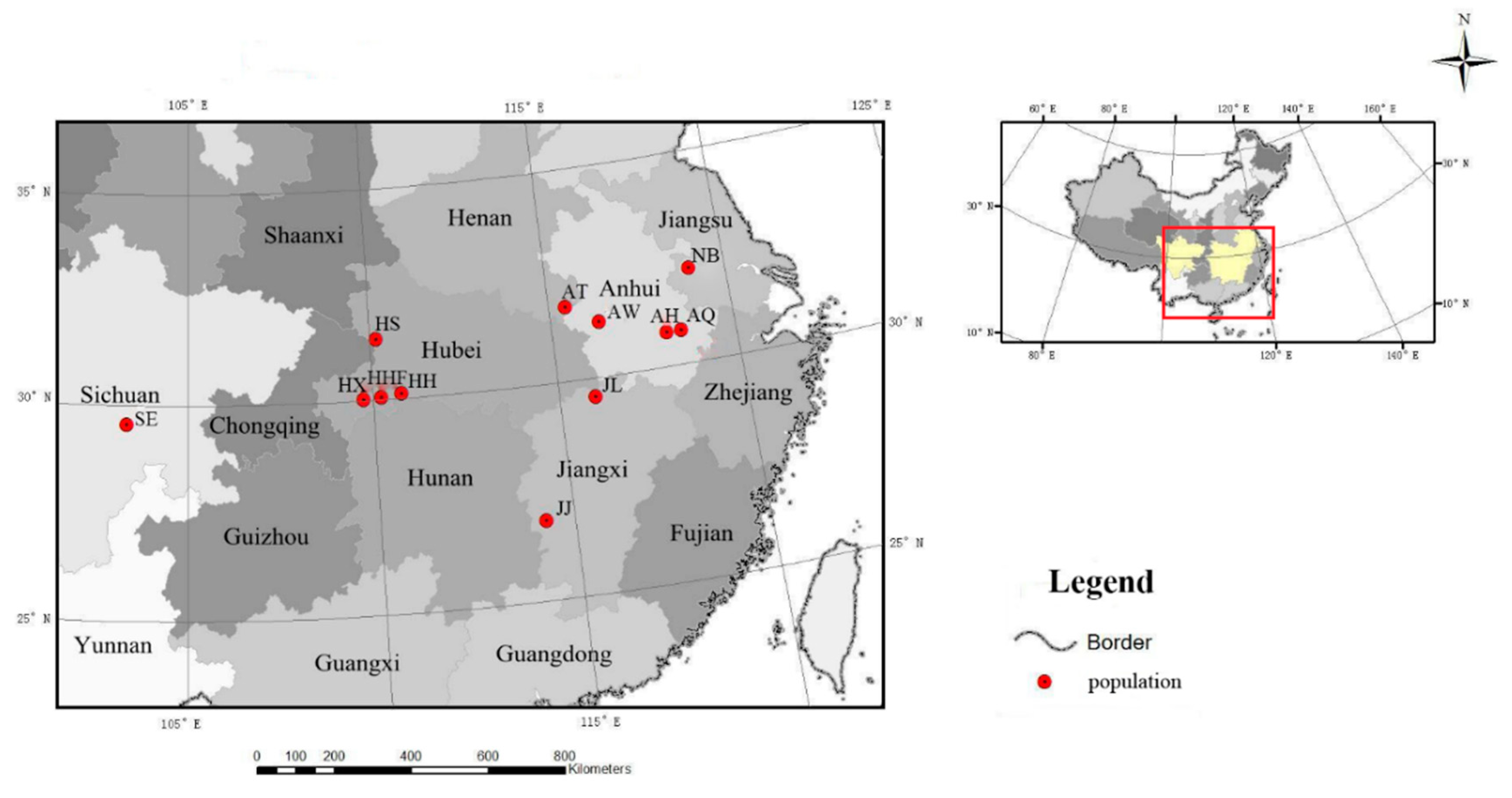
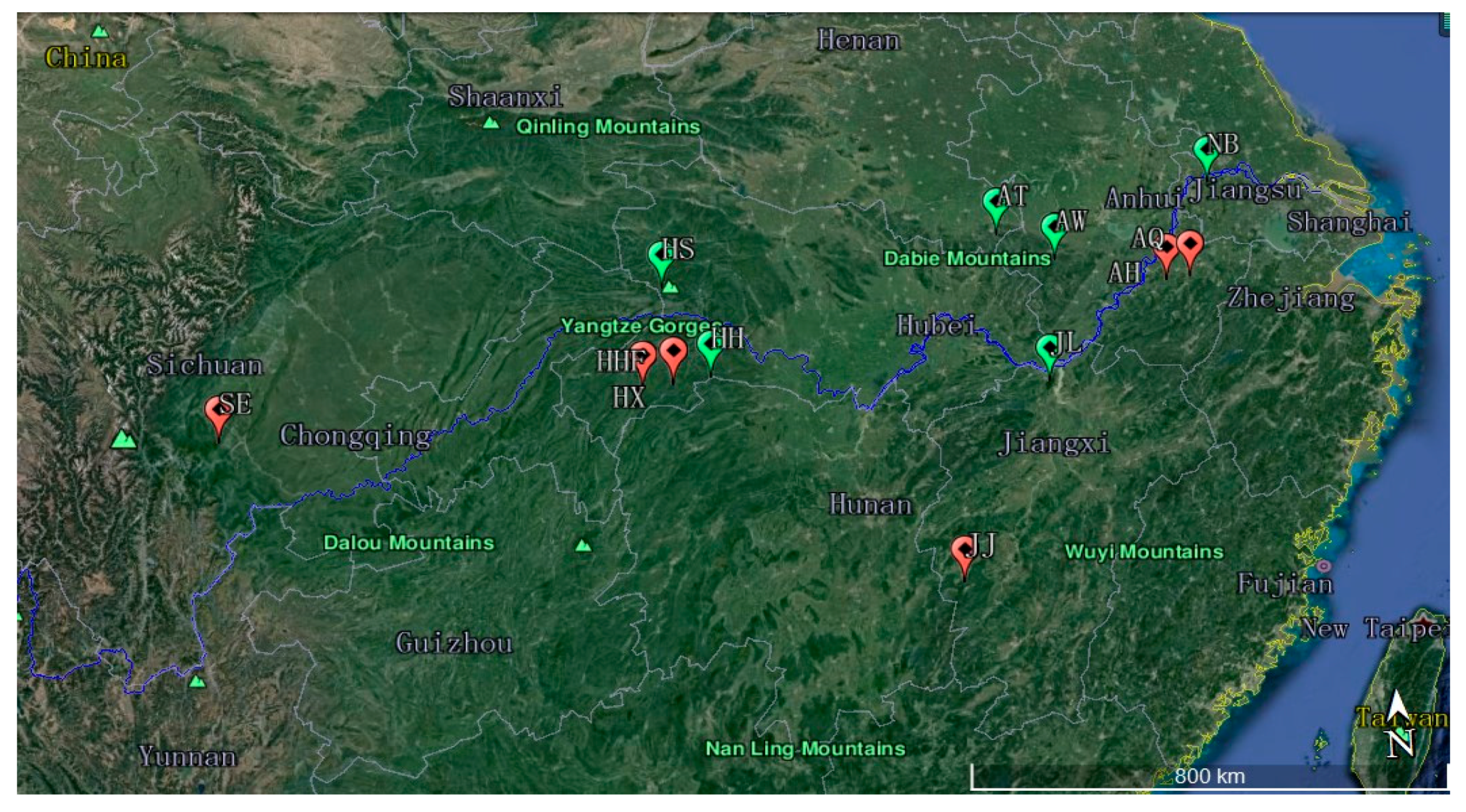
2.1. Sample Collection
2.2. DNA Extraction
2.3. ISSR Analysis
2.4. Data Analysis
3. Results
3.1. ISSR-Amplified Polymorphism
3.2. Genetic Diversity Analysis
3.3. Genetic Differentiation Analysis
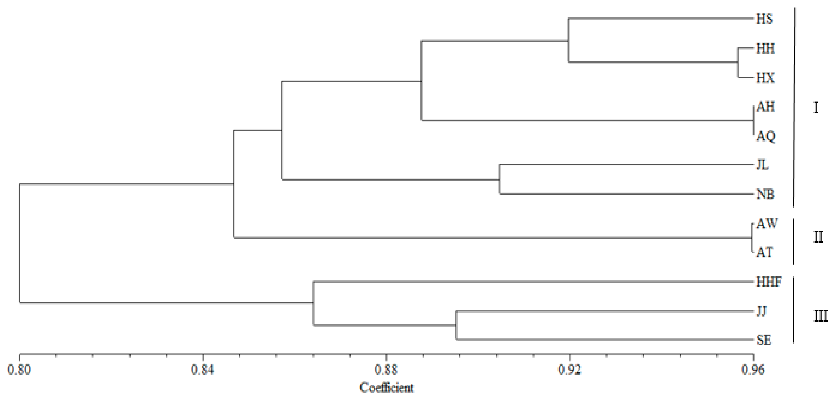
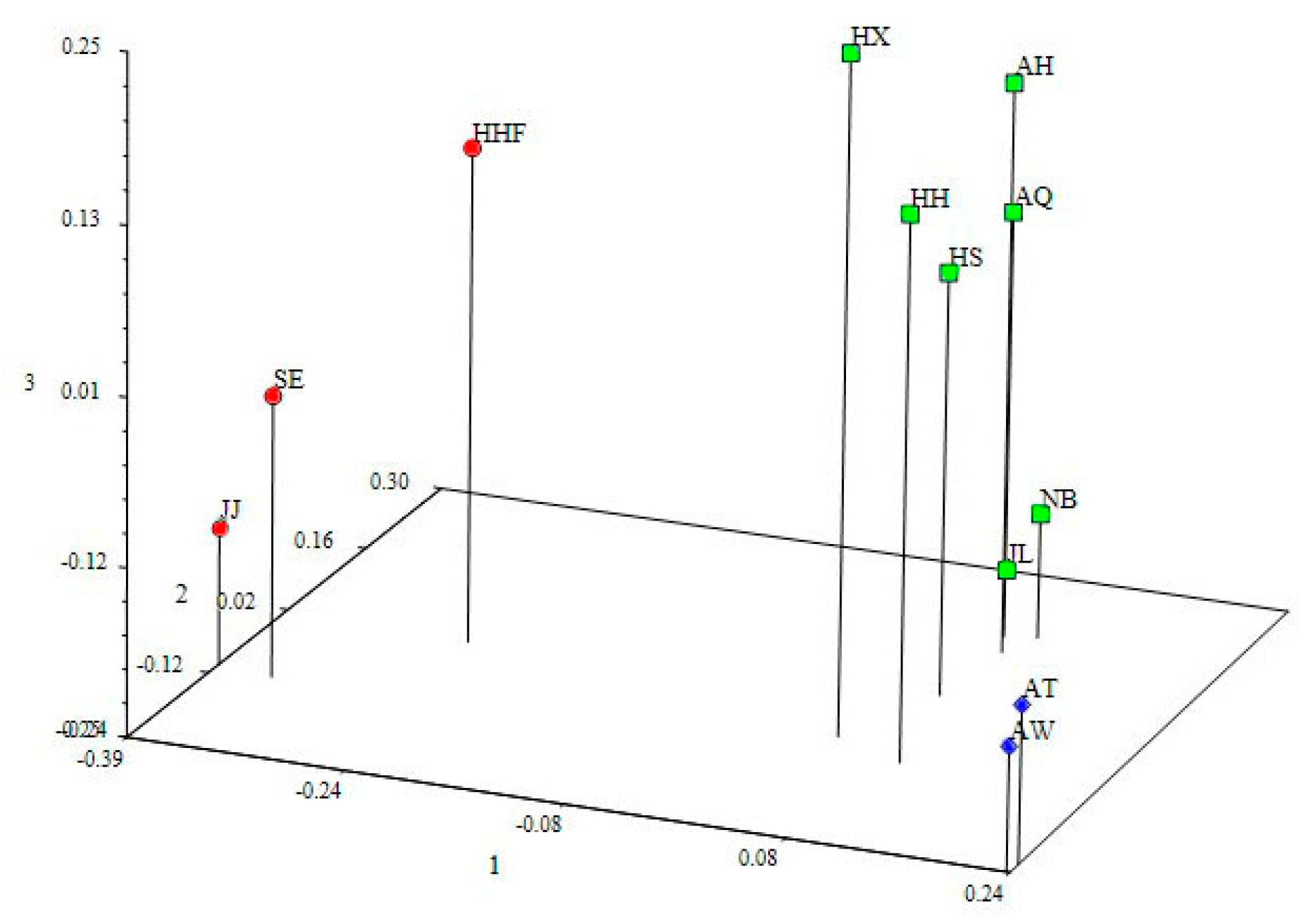
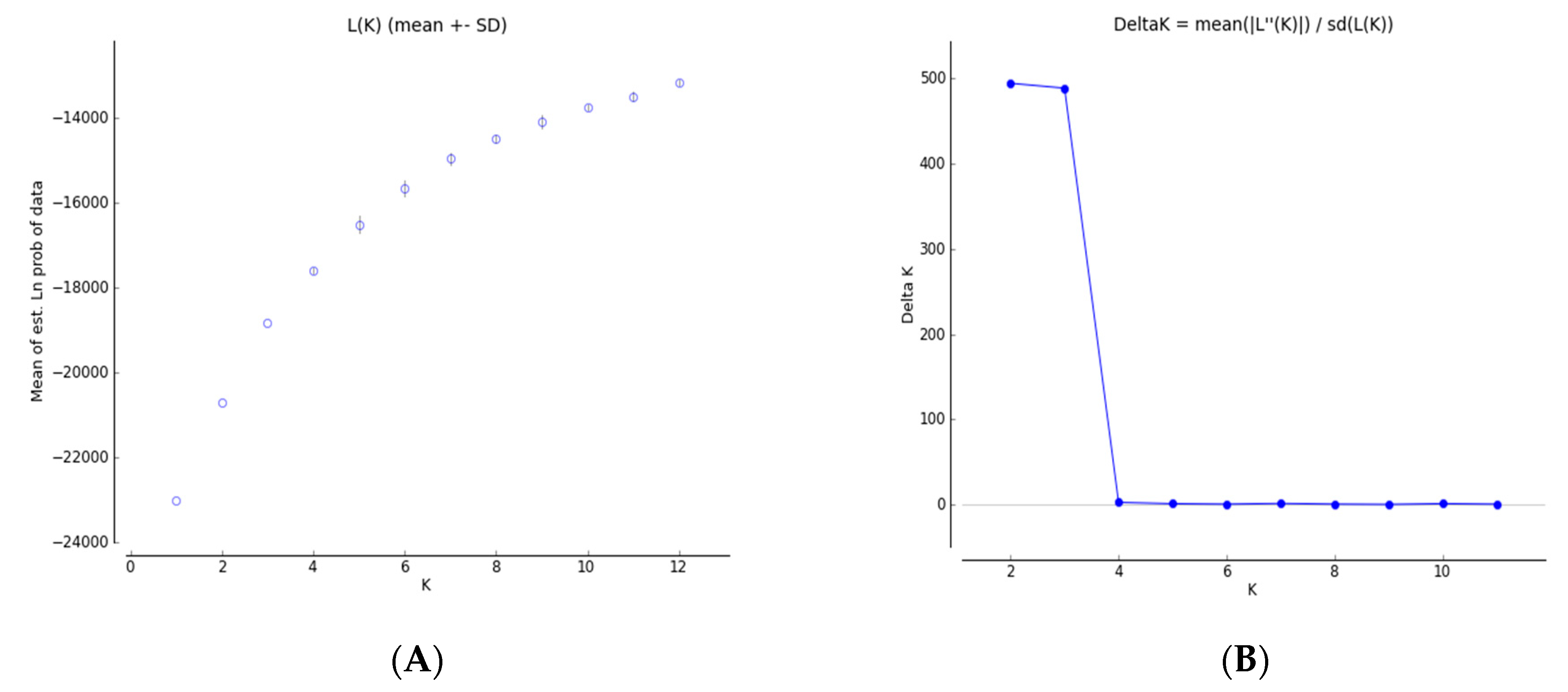
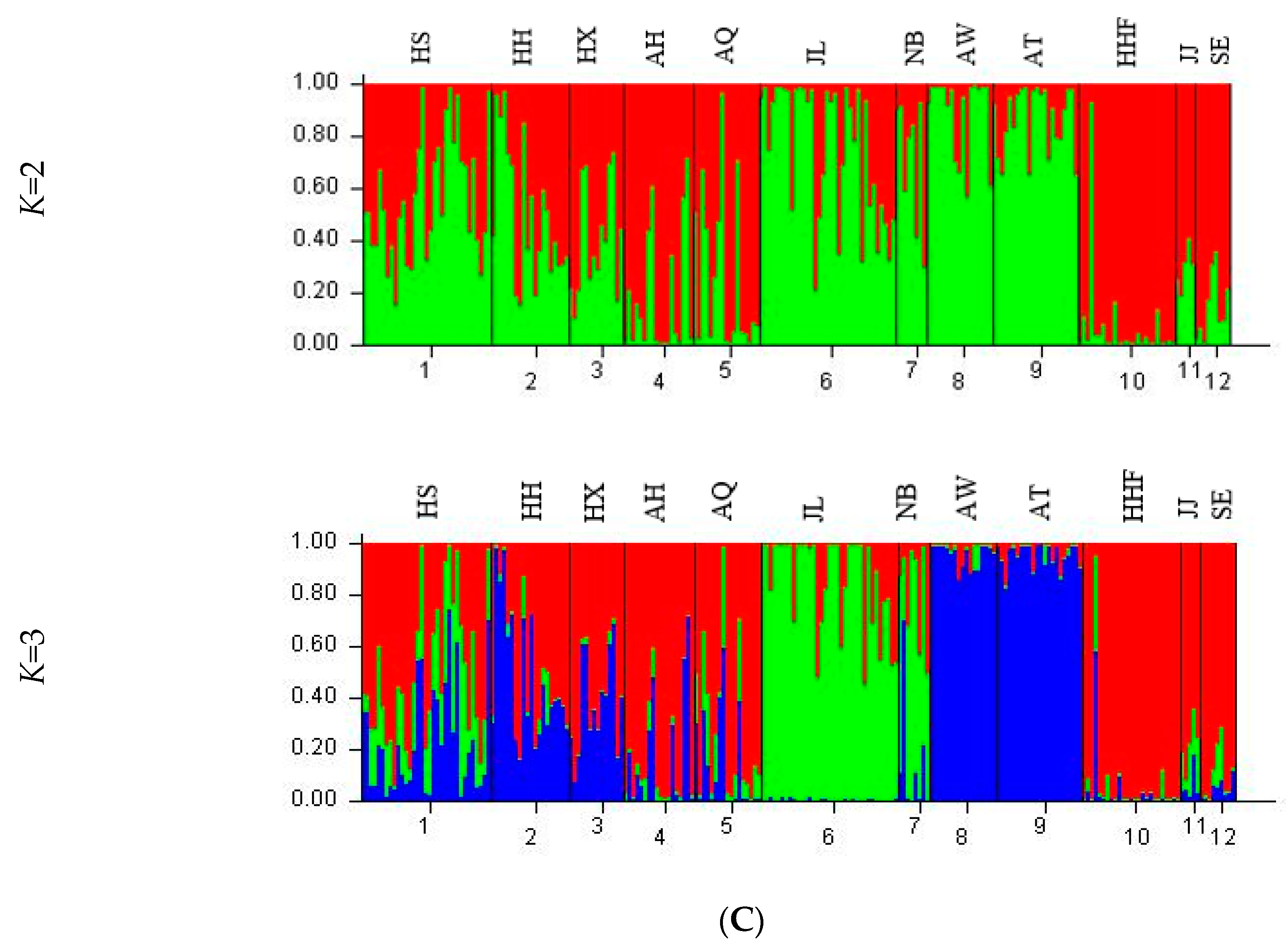
3.4. Genetic Structure and Genetic Relationship Analysis
4. Discussion
4.1. Genetic Diversity
4.2. Genetic Differentiation and Genetic Structure
4.3. Population Relationships
4.4. Genetic Conservation and Germplasm Utilization Strategy
5. Conclusions
Author Contributions
Funding
Acknowledgments
Conflicts of Interest
References
- Fu, X.X.; Liu, H.N.; Zhou, X.D.; Shang, X.L. Seed dormancy mechanism and dormancy breaking techniques for Cornus kousa var. chinensis. Seed Sci. Technol. 2013, 41, 458–463. [Google Scholar] [CrossRef]
- Xiao, D.Q.; Lu, C.X. Germplasm resource distribution and recent research advance in Dendrobenthamia multinervosa. J. Gansu For. Sci. Technol. 2008, 33, 24–25. [Google Scholar]
- Xiang, Q.Y. Cornales (Dogwood). In Encyclopedia of Life Sciences; John, W., Sons, L., Eds.; John Wiley & Sons Inc.: Hoboken, NJ, USA, 2005; pp. 1–4. [Google Scholar]
- Fu, X.X.; Xu, J.; Liu, G.H. The germplasm resources of ornamental flower and its development and utilization. Dev. For. Sci. Technol. 2015, 29, 1–6. [Google Scholar]
- Yang, C.H.; Wang, G.; Hou, N.; Zhou, J.W.; Chen, J. Study on the resources and utilization value of wild Dendrobenthamia plants in Guizhou Province. Seed 2013, 32, 61–68. [Google Scholar]
- Tang, J.J.; Liu, C.Y.; Shang, X.L.; Fu, X.X. Invitro culture and plant regeneration from stem segments of Dendrobenthamia angustata. Chin. Agric. Sci. Bull. 2014, 30, 79–83. [Google Scholar]
- Huo, D.; Deng, L.X.; Chen, J.Y.; Yang, C.H. Annual growth rhythm of Cornus kousa subsp. chinensis one-year-old seedling. Seed 2015, 34, 79–82. [Google Scholar]
- Zhou, J.; Dai, S.; Qian, C.M.; Su, Y.Y.; Li, S.X. Ultrastructure changes of eeed coat and endosperm on Cornus florida L. seed during dormancy breaking. J. Northeast For. Univ. 2016, 44, 34–38. [Google Scholar]
- Ker, K.R.; Bemmels, J.B.; Aitken, S.N. Low genetic diversity, moderate local adaptation, and phylogeographic insights in Cornus nuttallii. Am. J. Bot. 2011, 98, 1327–1336. [Google Scholar] [CrossRef]
- Hadziabdic, D.; Fitzpatrick, B.M.; Wang, X.; Wadl, P.A.; Rinehart, T.A.; Ownley, B.H.; Windham, M.T.; Trigiano, R.N. Analysis of genetic diversity in flowering dogwood natural stand using microsatellites: The effects of dogwood anthracnose. Genetica 2010, 138, 1047–1057. [Google Scholar] [CrossRef]
- Heikrujam, M.; Kumar, J.; Agrawal, V. Review on different mechanisms of sex determination and sex-linked molecular markers in dioecious crops: A current update. Euphytica 2015, 210, 161–194. [Google Scholar] [CrossRef]
- Zhao, N.; Yang, M.L.; Li, J.D.; Zheng, X.B.; Tan, B.; Ye, X.; Zhao, Z.H.; Feng, J.C. Core Germplasm Construction of Cornus officinalis by ISSR Markers. J. Agric. Biotechnol. 2017, 25, 579–587. [Google Scholar]
- Hassanpour, H.; Hamidoghli, Y.; Samizadeh, H. Estimation of genetic diversity in some Iranian cornelian cherries (Cornus mas L.) accessions using ISSR markers. Biochem. Syst. Ecol. 2013, 48, 257–262. [Google Scholar] [CrossRef]
- Ilczuk, A.; Jacygrad, E. In vitro propagation and assessment of genetic stability of acclimated plantlets of Cornus alba L. using RAPD and ISSR markers. Vitr. Cell. Dev. Biol.-Plant 2016, 52, 379–390. [Google Scholar] [CrossRef] [PubMed]
- Allen, G.C.; Flores-Vergara, M.A.; Krasynanski, S.; Kumar, S.; Thompson, W.F. A modified protocol for rapid DNA isolation from plant tissues using cetyltrimethylammonium bromide. Nat. Protoc. 2006, 1, 2320–2325. [Google Scholar] [CrossRef]
- Yeh, F.; Yang, R.; Boyle, T. POPGENE ver.1.32 Microsoft windows-based freeware for population genetic analysis. Cent. Int. For. Res. Univ. Alta. 1999, 110, 101–105. [Google Scholar]
- Peakall, R.; Smouse, P. GENALEX 6: Genetic analysis in Excel. Population genetic software for teaching and research. Mol. Ecol. Notes 2006, 6, 288–295. [Google Scholar] [CrossRef]
- Peakall, R.; Smouse, P. GenAIEx 6.5: Genetic analysis in Excel. Population genetic software for teaching and research: An update. Bioinformatics 2012, 28, 2537–2539. [Google Scholar] [CrossRef]
- Evanno, G.; Regnaut, S.; Goudet, J. Detecting the number of clusters of individuals using the software STRUCTURE: A simulation study. Mol. Ecol. 2005, 14, 2611–2620. [Google Scholar] [CrossRef]
- Falush, D.; Stephens, M.; Pritchard, J.K. Inference of population structure using multilocus genotype data: Dominant markers and null alleles. Mol. Ecol. Notes 2007, 7, 574–578. [Google Scholar] [CrossRef]
- Ma, W.H.; He, P.; Yuan, X.F.; Du, J.; Tian, L.H. Application of RAPD markers in phylogeny. J. Southwest Norm. Univ. (Nat. Sci. Ed.) 1999, 24, 482–491. [Google Scholar]
- Li, G.H.; Zhang, L.J.; Bai, C.K. Chinese Cornus officinalis: Genetic resources, genetic diversity and core collection. Genet. Resour. Crop Evol. 2012, 59, 1659–1671. [Google Scholar] [CrossRef]
- Yu, H.H.; Yang, Z.L.; Sun, B.; Liu, R.N. Genetic diversity and relationship of endangered plant Magnolia officinalis (Magnoliaceae) assessed with ISSR polymorphisms. Biochem. Syst. Ecol. 2011, 39, 71–78. [Google Scholar] [CrossRef]
- Luo, S.J.; He, Y.H.; Ning, G.G.; Zhang, J.Q.; Ma, G.Y.; Bao, M.Z. Genetic diversity and genetic structure of different populations of the endangered species Davidia involucrata in China detected by inter-simple sequence repeat analysis. Trees 2011, 25, 1063–1071. [Google Scholar] [CrossRef]
- Xie, G.W.; Peng, X.Y.; Zheng, Y.L.; Zhang, J.X. Genetic diversity of endangered plant Monimopetalum chinense in China detected by ISSR analysis. For. Sci. 2007, 43, 48–53. [Google Scholar]
- Call, A.; Sun, Y.X.; Yu, Y.; Pearman, P.B.; Thomas, D.T.; Trigiano, R.; Carbone, I.; Xiang, Q.Y. Genetic structure and post-glacial expansion of Cornus florida L. (Cornaceae): Integrative evidence from phylogeography, population demographic history, and species distribution modeling. J. Syst. Evol. 2016, 54, 136–151. [Google Scholar] [CrossRef]
- Wang, H.X.; Hu, Z.A. Plant breeding system, genetic structure and conservation of genetic diversity. Biodiversity 1996, 4, 92–96. [Google Scholar]
- Fischer, P. Time dependent flow in equimolar micellar solutions: Transient behaviour of the shear stress and first normal stress difference in shear induced structures coupled with flow instabilities. Rheol. Acta 2000, 39, 234–240. [Google Scholar] [CrossRef]
- Sokal, R.R.; Jacquez, G.M.; Wooten, M. Spatial autocorrelation analysis of migration and selection. Genetics 1989, 121, 845–855. [Google Scholar]
- Hamrick, J.L.; Godt, M.J.W. Allozyme diversity in plant species. In Plant Population Genetics, Breeding, and Genetic Resources; Brown, A.H.D., Clegg, M.T., Kahler, A.L., Weir, B.S., Eds.; Sinauer Associate Inc.: Cary, NC, USA, 1990; pp. 43–63. [Google Scholar]
- Reed, S. Self-incompatibility in Cornus florida L. HortScience 2004, 39, 335–338. [Google Scholar] [CrossRef]
- Zhang, Y.J.; Wang, Y.S. Genetic diversity of endangered shrub Reaumuria trigyna population detected by RAPD and ISSR markers. For. Sci. 2008, 241, 1455–1460. [Google Scholar]
- Rossell, I.M.; Rossell, C.R.; Hining, K.J.; Anderson, R.L. Impacts of dogwood anthracnose (Discula destructiva Redlin) on the fruits of flowering dogwood (Cornus florida L.): Implications for wildlife. Am. Midl. Nat. 2001, 146, 379–387. [Google Scholar] [CrossRef]
- Li, K.Q.; Chen, L.; Feng, Y.H.; Yao, J.X.; Li, B.; Xu, M.; Li, H.G. High genetic diversity but limited gene flow among remnant and fragmented natural populations of Liriodendron chinense Sarg. Biochem. Syst. Ecol. 2014, 54, 230–236. [Google Scholar] [CrossRef]
- Li, X.C.; Fu, X.X.; Shang, X.L.; Yang, W.X.; Fang, S.Z. Natural population structure and genetic differentiation for heterodicogamous plant: Cyclocarya paliurus (Batal.) Iljinskaja (Juglandaceae). Tree Genet. Genomes 2017, 13, 80. [Google Scholar] [CrossRef]
- Frankham, R.; Ballou, J.D.; Briscoe, D.A. Introduction to Conservation Genetics; Ambridge University Press: Cambridge, UK, 2002. [Google Scholar]
- Li, B.; Gu, W.C. Conservation genetics of Pinus bungeana—Evaluation and conservation of natural populations’ genetic diversity. Sci. Silvae Sin. 2005, 41, 57–64. [Google Scholar]
- Quevedo, A.A.; Schleuning, M.; Hensen, I.; Saavedra, F.; Durka, W. Forest fragmentation and edge effects on the genetic structure of Clusia sphaerocarpa and C. lechleri (Clusiaceae) in tropical montane forests. J. Trop. Ecol. 2013, 29, 321–329. [Google Scholar] [CrossRef]


| Population Code | Location | Number of Samples | Latitude (N) | Longitude (E) | Altitude (m) |
|---|---|---|---|---|---|
| HHF | Hefeng, Hubei | 25 | 30°03′29.27″ | 110°12′36.75″ | 1100~1526 |
| HX | Xuanen, Hubei | 14 | 30°01′52.07″ | 109°44′49.40″ | 1326~2016 |
| HS | Shennongjia, Hubei | 33 | 31°25′28.85″ | 110°10′17.44″ | 1100~2074 |
| AH | Huangshan, Anhui | 18 | 30°47′26.52″ | 118°6′19.87″ | 1162~1585 |
| AQ | Jixi, Qingliangfeng, Anhui | 17 | 30°47′40.20″ | 118°30′23.65″ | 700~1399 |
| AW | Shucheng, Wanfoshan, Anhui | 17 | 31°17′12.12″ | 116°19′59.59″ | 979~1400 |
| AT | Jinzhai, Tian Tang Zhai, Auhui | 22 | 31°44′42.00″ | 115°27′49.32″ | 990~1500 |
| SE | Leshan, Emei, Sichuan | 9 | 29°33′02.42″ | 103°21′45.21″ | 1120~1978 |
| HH | Shimen, Hupingshan, Hunan | 20 | 30°06′40.61″ | 110°46′44.27″ | 1100~2084 |
| NB | Nanjing, Baohua, Jiangsu | 8 | 32°07′45.54″ | 119°05′40.58″ | 200~300 |
| JJ | Ji’an, Jinggangshan, Jiangxi | 5 | 26°50′1.00″ | 114°15′42.00″ | 500~610 |
| JL | Jiujiang, Lushan, Jiangxi | 35 | 29°33′56.18″ | 115°57′36.22″ | 500~1350 |
| Primer | Sequences (5′~3′) | Temperature (°C) | Total Bands | Polymorphic Bands | Polymorphism (PPL) (%) |
|---|---|---|---|---|---|
| UBC808 | AGAGAGAGAGAGAGAGC | 52 | 12 | 12 | 100 |
| UBC809 | AGAGAGAGAGAGAGAGG | 52 | 9 | 9 | 100 |
| UBC820 | GTGTGTGTGTGTGTGTC | 57 | 14 | 14 | 100 |
| UBC823 | TCTCTCTCTCTCTCTCC | 57 | 9 | 9 | 100 |
| UBC836 | AGAGAGAGAGAGAGAGYA | 52 | 10 | 10 | 100 |
| UBC842 | GAGAGAGAGAGAGAGAYG | 56 | 10 | 10 | 100 |
| UBC846 | CACACACACACACACART | 55 | 10 | 10 | 100 |
| UBC847 | CACACACACACACACARC | 57 | 7 | 7 | 100 |
| UBC849 | GTGTGTGTGTGTGTGTYA | 57 | 6 | 6 | 100 |
| UBC864 | ATGATGATGATGATGATG | 56 | 7 | 7 | 100 |
| Total | / | / | 94 | 94 | 100 |
| Population Code | Nei’s Genetic Diversity (He) | Shannon Information Index (I) | Percentage of Polymorphic Loci (PPL, %) |
|---|---|---|---|
| HHF | 0.247 | 0.370 | 72.34 |
| HX | 0.190 | 0.283 | 56.38 |
| HS | 0.220 | 0.336 | 73.40 |
| AH | 0.288 | 0.423 | 75.53 |
| AQ | 0.272 | 0.401 | 72.34 |
| AW | 0.177 | 0.274 | 60.64 |
| AT | 0.221 | 0.331 | 65.96 |
| SE | 0.245 | 0.357 | 62.77 |
| HH | 0.229 | 0.353 | 78.72 |
| NB | 0.211 | 0.315 | 58.51 |
| JJ | 0.205 | 0.301 | 53.19 |
| JL | 0.199 | 0.304 | 65.96 |
| Population level | 0.226 | 0.338 | 66.31 |
| Species level | 0.333 | 0.504 | 100.00 |
| Source of Variation | df | Sum of Squares | Mean Squares | Variance Components | Percentage of Variance Components | Statistics | Value |
|---|---|---|---|---|---|---|---|
| Among pops | 11 | 1514.01 | 137.64 | 6.95 | 38.45% | PhiPT | 0.3845 |
| within pops | 211 | 2348.52 | 11.13 | 11.13 | 61.55% | ||
| Total | 222 | 3862.53 | 148.77 | 18.08 | 100.00% |
| Pop | HS | HH | HX | AH | AQ | JL | NB | AW | AT | HHF | JJ | SE |
|---|---|---|---|---|---|---|---|---|---|---|---|---|
| HS | *** | 0.928 | 0.915 | 0.886 | 0.896 | 0.866 | 0.890 | 0.867 | 0.863 | 0.858 | 0.785 | 0.819 |
| HH | 0.075 | *** | 0.960 | 0.887 | 0.887 | 0.816 | 0.869 | 0.896 | 0.879 | 0.851 | 0.791 | 0.817 |
| HX | 0.089 | 0.041 | *** | 0.891 | 0.879 | 0.790 | 0.849 | 0.843 | 0.848 | 0.861 | 0.780 | 0.824 |
| AH | 0.121 | 0.120 | 0.116 | *** | 0.964 | 0.823 | 0.866 | 0.821 | 0.842 | 0.835 | 0.763 | 0.796 |
| AQ | 0.109 | 0.120 | 0.129 | 0.037 | *** | 0.861 | 0.908 | 0.840 | 0.852 | 0.845 | 0.790 | 0.806 |
| JL | 0.144 | 0.204 | 0.235 | 0.195 | 0.150 | *** | 0.903 | 0.787 | 0.782 | 0.795 | 0.759 | 0.762 |
| NB | 0.116 | 0.140 | 0.164 | 0.144 | 0.097 | 0.102 | *** | 0.850 | 0.851 | 0.814 | 0.776 | 0.798 |
| AW | 0.143 | 0.110 | 0.171 | 0.198 | 0.175 | 0.239 | 0.162 | *** | 0.963 | 0.765 | 0.746 | 0.768 |
| AT | 0.147 | 0.129 | 0.165 | 0.173 | 0.161 | 0.246 | 0.162 | 0.038 | *** | 0.771 | 0.743 | 0.765 |
| HHF | 0.153 | 0.162 | 0.149 | 0.180 | 0.169 | 0.229 | 0.206 | 0.268 | 0.260 | *** | 0.849 | 0.877 |
| JJ | 0.242 | 0.235 | 0.248 | 0.271 | 0.235 | 0.276 | 0.254 | 0.294 | 0.297 | 0.164 | *** | 0.896 |
| SE | 0.200 | 0.202 | 0.193 | 0.228 | 0.216 | 0.272 | 0.226 | 0.264 | 0.268 | 0.131 | 0.110 | *** |
| Population | K = 2 | K = 3 | |||
|---|---|---|---|---|---|
| 1 (red) | 2 (green) | 1 (red) | 2 (green) | 3 (blue) | |
| HS | 0.4328 | 0.5672 | 0.5103 | 0.2539 | 0.2357 |
| HH | 0.4951 | 0.5049 | 0.4815 | 0.0351 | 0.4835 |
| HX | 0.5934 | 0.4066 | 0.6059 | 0.0140 | 0.3801 |
| AH | 0.8147 | 0.1853 | 0.8130 | 0.0342 | 0.1529 |
| AQ | 0.7381 | 0.2619 | 0.7306 | 0.1306 | 0.1388 |
| JL | 0.2451 | 0.7549 | 0.1415 | 0.8511 | 0.0074 |
| NB | 0.2873 | 0.7127 | 0.1911 | 0.6611 | 0.1477 |
| AW | 0.1040 | 0.8960 | 0.0260 | 0.0193 | 0.9547 |
| AT | 0.1301 | 0.8699 | 0.0362 | 0.0120 | 0.9518 |
| HHF | 0.9288 | 0.0712 | 0.9328 | 0.0300 | 0.0372 |
| JJ | 0.7018 | 0.2982 | 0.7782 | 0.1590 | 0.0628 |
| SE | 0.8489 | 0.1511 | 0.8998 | 0.0556 | 0.0446 |
© 2019 by the authors. Licensee MDPI, Basel, Switzerland. This article is an open access article distributed under the terms and conditions of the Creative Commons Attribution (CC BY) license (http://creativecommons.org/licenses/by/4.0/).
Share and Cite
Yuan, J.-Q.; Fang, Q.; Liu, G.-H.; Fu, X.-X. Low Divergence Among Natural Populations of Cornus kousa subsp. chinensis Revealed by ISSR Markers. Forests 2019, 10, 1082. https://doi.org/10.3390/f10121082
Yuan J-Q, Fang Q, Liu G-H, Fu X-X. Low Divergence Among Natural Populations of Cornus kousa subsp. chinensis Revealed by ISSR Markers. Forests. 2019; 10(12):1082. https://doi.org/10.3390/f10121082
Chicago/Turabian StyleYuan, Jia-Qiu, Qin Fang, Guo-Hua Liu, and Xiang-Xiang Fu. 2019. "Low Divergence Among Natural Populations of Cornus kousa subsp. chinensis Revealed by ISSR Markers" Forests 10, no. 12: 1082. https://doi.org/10.3390/f10121082
APA StyleYuan, J.-Q., Fang, Q., Liu, G.-H., & Fu, X.-X. (2019). Low Divergence Among Natural Populations of Cornus kousa subsp. chinensis Revealed by ISSR Markers. Forests, 10(12), 1082. https://doi.org/10.3390/f10121082