Article

Spatial Patterns in Different Stages of Regeneration after Clear-Cutting of a Black Locust Forest in Central China

1
Key Laboratory for Silviculture and Conservation, Ministry of Education, Beijing Forestry University, Beijing 100083, China
2
National Energy R&D Center for Non-food Biomass, Beijing Forestry University, Beijing 100083, China
3
College of Forestry, Jiangxi Agricultural University, Nanchang 330045, China
4
Beijing Advanced Innovation Center for Tree Breeding by Molecular Design, Beijing Forestry University, Beijing 100083, China
*
Author to whom correspondence should be addressed.
Forests 2019, 10(12), 1066; https://doi.org/10.3390/f10121066
Submission received: 30 October 2019 / Revised: 19 November 2019 / Accepted: 22 November 2019 / Published: 24 November 2019
(This article belongs to the Section Forest Ecology and Management)

Abstract

:
Estimating underlying mechanisms and dynamics from observed tree patterns can provide guidance for plantation management. Robinia pseudoacacia can reproduce via clonally produced ramets, leading to a complex distribution of stems. Three second generation plots and three third generation plots (each plot 50 m × 50 m) were established across a wide age range after clear-cutting in a Robinia pseudoacacia plantation in central China. We measured spatial coordinates, diameter at breast height (DBH) or diameter at basal stem, and heights of all recruits, as well as the coordinates and base diameter of all stumps, in six plots. The spatial pattern in different plots and the spatial relation between stumps and regenerations after clear-cutting were analyzed. To estimate the underlying processes of the observed patterns, we fitted Matérn and Variance-Gamma cluster processes to the observed dataset. The results revealed that the percentage of ramets from stumps decreasing with age in the two types of stands (from 40.4% to 30.1%, from 57.6% to 35.7%), and trees exhibited an aggregated distribution in all plots, but the degree of aggregation exhibited a decreasing trend with age, and aggregation occurred at different scale. Furthermore, a large proportion of ramets had their nearest neighbor at a short distance (<1 m) based on analysis of the nearest neighbour function. The bivariate analysis revealed that the spatial relation between stumps and ramets changed with age, and a repulsion trend was found between them in all the six plots. The Variance-Gamma process with covariate of Cartesian coordinates fitted the observed patterns better than others. The observed pattern was likely driven by root dispersal limitation, seed dispersal limitation, human disturbance, and intraspecific competition. Spatial patterns are important characteristics in forest stand structure, and understanding the pattern change and its underlying mechanisms could allow for better timing of artificial disturbances to optimize stand structure and promote stand growth.

1. Introduction

Regeneration plays a vital role during forest ecosystem restoration and sustainable management. It is essential to understand natural regeneration processes for economic and ecological reasons [1]. Logging of natural forests over the last century has led to large areas of artificial forests and semi-natural forests. Different cutting methods effects on the processes and spatial patterns of regeneration. For example, retaining tree when clear-cutting could increase the structural diversity [2], and natural regeneration could be improved by commercial thinning [3]. Additionally, the shelterwood system can help prevent high losses of soil nitrogen during the start of regeneration [4], and appropriate regeneration can be ensured after combining seed-tree harvesting with the shelterwood and scarification in black spruce stands [5]. These studies have focused on regeneration growth, but there is a lack of understanding about spatial patterns and regeneration processes after anthropogenic disturbances such as clear-cutting and tending-felling.
Black locust (Robinia pseudoacacia L.) is a tree species native to the Appalachian Mountains of North America with a relatively short lifespan; there it plays an important role in early primary successional series [6]. In the 1960s, the black locust was introduced to Luoning (Henan Province, China) from North Korea and planted widely in a local hilly region [7] for erosion control, eco-environmental construction, and its economic benefits; due to its nitrogen-fixing ability and its asexual regeneration capacity [6,8], the black locust can grow well in an infertile environment. The black locust has been planted widely in China for soil and water conservation [9] and is now a widespread exotic tree species, covering more than 26,635 hectares in the Luoning region. Although it may effect plant assemblages [10], the ecosystem and recruitment of native species [11], and may cause both a loss in plant richness and shifts in species composition [12,13], the black locust is now considered a promising tree for reforestation [10,14] and soil conservation. The pure black locust stands in Luoning region grew well initially, without any artificial management of water or fertilizer, but several clear-cutting events for timber utilization led to a change in forest structure. Clear-cutting is the main logging method for black locust forests in the Luoning region and a widespread forest harvesting method in other places [15]. However, higher temperatures and wind exposure following clear-cutting can cause large shifts in microclimates [16], which can lead to different habitat that may have a strong effect on regeneration and lead to highly fragmented landscapes [5]. Clear-cutting can also lead to defoliation of conifer regeneration affected by spruce budworm (Choristoneura fumiferana) due to a lack of shelterwood [17]. Black locust trees regenerate asexually through the formation of new ramets on cut stumps and residual horizontal roots after clear-cutting [8]. In the hybrid aspen plantation forest, management strategies for root sucker stands are important for the outcome [18], so the study the root suckers in black locust plantation forest is necessary. Efficient and sustainable utilization of black locust requires that forest management applies silviculture practices that mimic natural forest structures and processes to protect the ecological structure and function of the forest [19,20]. The natural processes that generate and maintain spatial distribution patterns have long been of great interest [21] and include a deeper understanding of regeneration processes [14] and the spatial distribution of regeneration following logging. The problem of pattern and scale is of great importance and is one of the central topics in ecology [22,23,24]. Nevertheless, understanding the underlying biological process from the observed pattern remains a challenge [25,26] because the observed pattern has been modified by combinations of various past events over a long period and at various spatial scales, especially in forests [19,25]. Most tree species in forests worldwide are spatially aggregated at different scales and the spatial patterns of trees change with the developmental stage of the forest, particularly in natural forests not heavily disturbed by humans [23,27,28,29]. Several studies have focused on the spatial patterns of trees according to forest development stage [30,31,32], some studies manifested that radial growth of trees and tree growth model was affected significantly by tree spatial position relative to skidding trails in conifer forest after different cutting methods [33,34]. Few have explored the spatial patterns of planted black locust forests in different growth stages, such as intergenerational stages and age stages that have been disturbed by tending-felling and clear-cutting.
To characterize spatial patterns and processes of regeneration of black locust trees in different growth stages following logging, spatial point pattern analysis was used to detect black locust forest structure. Forest structure has been measured by a range of methods, such as the uniform angle index [35], mingling index [36], and dominance index [37], all of which are based on neighborhood trees without the exact position of every tree. Spatial functions such as Ripley’s K function [38,39,40] and Ripley’s L function [41], which is a transformation of K to stabilize the variance of the estimator and make it easier to assess deviations [42], have the advantage of providing a ‘plant’s eye view’ to normalize the average density of individuals surrounding the focal plant at a given distance [43,44]. We will use g(r) function in this study, which has become more and more popular in ecology [26,45], and. Summary spatial statistics are not sufficient to provide a direct link between underlying ecological processes and spatial patterns, but by fitting point process models to observing patterns, we can adjust for effects that might otherwise distort the analysis and obtain additional insights about the relationship [26,42,46].
The objectives of this study were to address the following questions:
(1)
What are the regeneration spatial patterns of black locust trees in different growth stages following logging?
(2)
What is the spatial relation between stumps and regenerations?
(3)
What are the ecological processes behind these spatial patterns?
We hypothesized that:
(1)
The extent of cluster of spatial pattern will show a downward trend with age due to impact of self-thinning and tending.
(2)
Spatial repulsion between stumps and ramets will happen at small scales, because sprouts of stumps suppress sprouts of roots and seedlings.
(3)
Silvicultural scheme, expansion and extension characteristics of black locust, and grazing will be the ecological processes behind these spatial patterns.

2. Materials and Methods
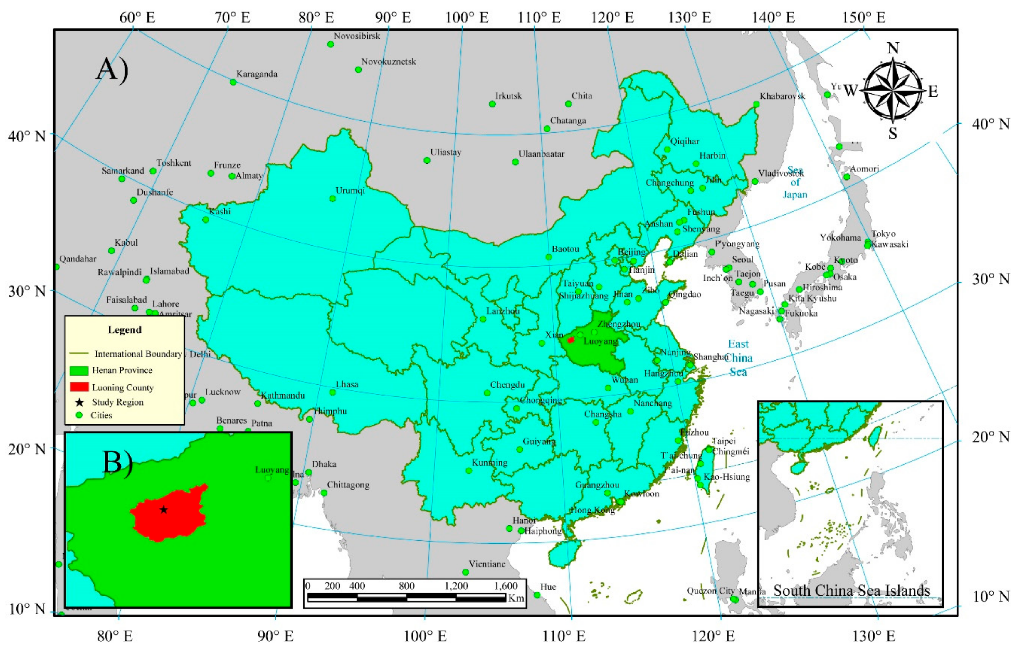
2.1. Study Area

Our study was conducted in a government-owned forest farm located in Henan Province (Figure 1), central China (34°05′–34°38′ N, 111°08′–111°49′ E). The elevation of the study area varies from 650–770 m a.s.l., and the climate is a warm temperate continental monsoon climate with an average annual temperature of 13.7 °C (min. −21 °C and max. 42 °C) and an annual precipitation of 552 mm. The soil is mainly brown earth [7].
The flora in the study area belongs to the Chinese–Japanese plant sub-region of the Pan-Arctic plant region. Native plants mainly include plants in the families Salicaceae, Betulaceae, Juglandaceae, Aceraceae, Rosaceae, Ranunculaceae, and Fagaceae. The black locust plantation at our study site was developed by stem-cut reforestation from seedlings in the 1960s with an initial stocking density of approximately 40,000 stems ha−1 (0.5 m × 0.5 m). During the growing process over the decades before wood harvesting, several tending events were carried out to adjust the stand density to promote forest growth. After wood harvesting by clear-cutting, each of the original parent trees (stumps) gave rise to a group (or cluster) of young trees. The observed pattern of young trees is the superposition of the clusters originating from the different parents. R. pseudoacacia can spread locally at rates up to 1 m per year [47]. The shrub layer usually contains Vitex negundo L., Ziziphus jujuba Mill., and some others.

2.2. Experiment Design and Data Collection

Six black locust stands that had experienced clear-cutting were selected in 2017. The stands were characterized as two types: (1) second generation R. pseudoacacia stand and (2) third generation R. pseudoacacia stand. We established six 50 m× 50 m plots (II-4, II-6, II-9, III-1, III-5, III-8), each plot was more than 50 m from the road and the margin of stands to avoid the edge effect, and had an average slope of less than 5° (Figure 2). All plots were located in a similar environment, with primarily cinnamon soil, N-S orientation, and similar herbaceous vegetation type, the mean inclination is <5 °C. Plots II-4, II-6, II-9 and plots III-1, III-5, and III-8 represent 4, 6, and 9 years after the first clear-cutting and 1, 5, and 8 years after the second clear-cutting, respectively. No management activities were undertaken in plots II-4, III-1, III-5, and III-8, and there was no grazing in these plots. However, plots II-6, and II-9, had been disturbed by cattle browsing after the forest tending (non-commercial thinning) was conducted every four years. Characteristics of all plots are presented in Table 1.
Asexual reproduction arising from adventitious buds on roots and stumps (root sprouting and stump sprouting) is the primary regeneration mode of black locust after clear-cutting [6,8,48,49] and constitutes 86–95% of the net primary productivity [50]. Seedlings were regenerated in the spring following clear-cutting; regeneration continued for several years, and then faded out thereafter [8]. The plots had only small amounts of shrub (Vitex negundo L.; 1–6%) and other trees (Ailanthus altissima; <0.5%) (Figure 2), and the stands were almost exclusively comprised of R. pseudoacacia. The positions of all live trees and stumps within each plot were recorded. To simplify the field work, we established a unified coordinate system with the north–south orientation as the y-axis, the east–west orientation as the x-axis, and the southwest corner as the origin of the coordinate system. Each plot was divided into a regular grid of 5 × 5 m to investigate the regeneration [19,51], a tape and a metal ruler were used to measure the X/Y coordinates. We measured the diameter at breast height (DBH; 1.3 m) of each tree, except at plot III-1 where the trees were too small so the diameter at base stem was measured instead of DBH. Ramets sprouted from cut stumps were clumped, so we only measured the height and DBH (or diameter at base stem) of these trees after the positions of the stumps were located.

2.3. Data Analysis

2.3.1. Analysis of Basic Stand Characteristics

To describe the spatial distribution of trees visually, a scatter diagram of trees of the six plots was created (Figure 2), and the diameter distribution was analyzed in the six plots. Data analysis and plotting were implemented using R software version 3.3.1 with the ggplot2 package [52,53].

2.3.2. Correlation and Spacing Analysis

It was difficult to discriminate root sprouts and seedlings in the R. pseudoacacia stands; therefore, for convenient data description, we used the abbreviation SR to represent trees sprouted from roots or seedlings and the abbreviation SS to represent trees sprouted from stumps. The univariate function K(r), which has become established across wide areas following Ripley’s influential paper [39], however the K(r) function is a cumulative measure for detecting aggregation or dispersion up to a given distance r [42,45,54], so the larger distance effects would be affected by a shorter distance of r [23,55]. We used pair correlation function g(r) with Ripley’s isotropic edge correction to explore the fine-scale patterns of each plot, and g(r) = K’(r)/2πr, and K’(r) = (W/(n × (n − 1)) × sum[i,j] 1 {dij ≤ r}eij, and where r is the radius of each tree i, n is the number of plants in the researched plot, W is the area of the plot in m2, dij is the distance between plants i and j, {dijr} is an indicator that equals 1 if the distance is less than or equal to r, and eij is a weighting factor to correct for edge effects [42,56]. The univariate g(r) function can be used to test whether the spatial pattern of trees is random, clustered, or regular, and to describe the spatial scale range in which the patterns occur; thus, it can measure the correlation between trees. We also estimated the shortest distance of the spatial patterns based on the nearest neighbor function G(r), where G(r) = sum[i] I {di r}/n. In this equation, r is the distance, n is the number of points within the given pattern, di is the distance from point i to its nearest neighbor, and I(di < r) is an indicator function that equals 1 if the argument is true and 0 otherwise [57]. To explore spatial relationships between SR and stumps, bivariate spatial pattern analyses were performed using g12(r): g12(r) = K12(r)/2πr. The interpretation of the parameters is similar to that of the univariate g(r), which was used in many studies of spatial pattern [19,26,29,58].
We assumed that the plots were environmentally homogeneous because of the small size of the 0.25-ha plots, so we tested the observed values of g(r) and G(r) against the null model of complete spatial randomness (CSR) to analyze the underlying biological processes that generated the spatial patterns of R. pseudoacacia trees. We constructed a simulation envelope by calculating 999 Monte Carlo (MC) simulation patterns of a CSR null model and removed the five highest and five lowest values of the simulations. Values of g(r) and G(r) outside of the envelope were deemed different than the simulated null model: g(r) > 1 or g(r) < 1 when the pattern tends to aggregate or be regular, respectively [41], and values of G(r) above the theoretical value of the null model indicate that nearest-neighbor distances in the data are shorter than expected for a completely random pattern, which is consistent with clustering [42]. The significance of g12(r) was tested based on the null hypothesis of independence and keeping the stumps at fixed positions, g12(r) has an expectation of 1 under population independence but becomes bigger than 1 or smaller than 1 when two populations exhibit attraction or repulsion, respectively [26]. We used 999 simulations and the same procedure as described above for the univariate analysis. In order to analyze the distribution of SR around stumps, the numbers of SR at different distances from the stumps was calculated in each plot.

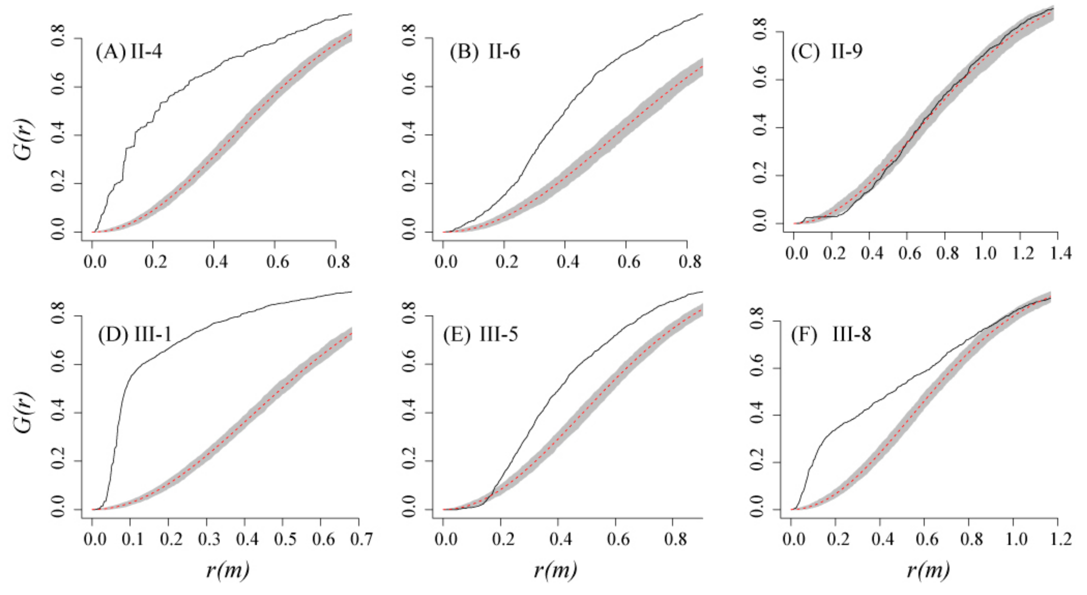
2.3.3. Fitting the Cluster Point Process to the Regeneration Data

Summary functions such as g(r) and G(r) are not sufficient to explain the underlying ecological process of spatial patterns, so we fitted appropriate cluster processes that can be interpreted biologically to our regeneration data. We applied the Matérn cluster process [59] and Variance-Gamma cluster process [60] to our data. Models were classified as with covariates and without covariates, and the log-quadratic of Cartesian coordinates x and y served as spatial covariates [42]. The Matérn cluster and Variance-gamma processes without covariate (also called Homogeneous Thomas process) described processes of dispersal limitation in which offspring are limited to aggregate around their parent trees [61], which is indicative of the neutral theory of tree distribution. The Matérn cluster and Variance-Gamma processes with covariate (also called Heterogeneous Thomas process) describe joint effects of dispersal and habitat heterogeneity, which reflect the neutral theory and niche theory of tree distribution respectively. Both of the cluster processes consist of a number of stochastic and independent so-called parents with given intensity κ, and the patterns follow a homogeneous Poisson process. Then, each parent point gives rise to a random number of offspring according to a Poisson distribution with mean µ offspring per parent. The offspring points are independent and identically distributed around each parent, with a spatial probability density depending only on the distance from offspring to parent. In the Matérn cluster process, offspring trees are distributed according a bivariate Gaussian distribution around parents, and the probability density of distance from parents decreases rapidly after a specific distance. The probability density of offspring of Variance-Gamma process has a heavy tail with function:
h u = 1 2 ν + 1 π η 2 Γ ν + 1 u η ν K ν u η
η is the scale parameter and ν is an extra parameter controlling the ‘shape’ of the density, which must satisfy ν > −1/2 [42].
Minimum contrast estimation with the K function was used to fit the processes to our observed data. The method of minimum contrast is measured by a function D(ψ), which denotes the contrast between the fitted curve and the empirical curve, where
D ψ = a b K ψ r K ^ r 2 d r
a and b are the limits of the range of distances considered, and Kψ(r) and K ^ r are the K function of the model and the empirical data, respectively [42]. Appropriate parameters of the model were searched to minimize the D(ψ). We used the K function to improve the quality of estimates in the method of minimum contrast.
The L function is a valuable tool for goodness-of-fit tests in point process statistics [54]. To test the deviation between the process that we modeled and our observed data, we used MC simulation envelopes generated by the cluster processes based on the L function of the models. The envelope limits were constructed by removing the five highest and five lowest values of L(r) among 999 random simulations based on the fitted processes. All spatial analyses were performed using spatstat package of the statistical software R version 3.3.1 and visual analyses were preformed using ggplot2 package [42,52].

3. Results

3.1. Basic Stand Characteristics

The number of R. pseudoacacia recruits varied from 1300 (plot II-9) to 5171 (plot III-1), and the mean diameter varied from 1.34 cm (±0.61 SD, plot III-1, diameter at basal stem) to 5.32 cm (±1.68 SD, plot II-9, DBH). The diameter distribution of R. pseudoacacia in all plots showed a slight left-skewed normal distribution. The proportion of SS decreased from 40.4% (II-4) to 30.1% (II-9) in second generation stands and decreased from 57.1% (III-1) to 35.7% (III-8) in third generation stands (Figure 3). The tree height varied from 1.89 ± 0.92 m (III-1) to 7.35 ± 2.68 m (III-8) in the 6 plots. The number of stumps in second generation stands was less than that in third generation stands (Figure 2); the mean base diameter of stumps was 15.31 ± 5.43 cm and 9.56 ± 2.83 cm in second and third generation stands respectively. The plots contained a small number of other trees; most of these were Vitex negundo L., which ranged in number from 44 (III-8) to 207 (II-4). We removed these trees from our data during statistical analyses.

3.2. Correlation and Spacing Analysis

The univariate g(r) function indicated that clustering of stems occurred at different scales in the six plots. The degree of clustering was highest in plot III-1, which was in its first year after the second clear-cutting (Figure 4). Increasing age of the plot showed decreasing percentages of cluster spatial distribution from 100% (in III-1) to 19.3% (in II-9), while the percentages of the random spatial distribution showed an increasing trend with increasing age, from 0 (in III-1) to 73.2% (in II-9) (Figure 5). Plot II-4 was significantly clustered at scales less than 4.8 m and scales around 5.6 m, and weakly distributed or random clustered thereafter. Only plot II-9 had regular spacing at short distances to up to 0.3 m, while the other plots exhibited an aggregation pattern at small scales. We found that spatial repulsion mainly happened at larger scales (>3 m) in plots II-4, II-6 and III-8 (Figure 4). The nearest neighbor function G(r) indicated that a substantial proportion of recruits had their nearest neighbor at a short distance and were distributed as heavily clustered at the small scale of 1 m, except plot II-9. In particular, almost all recruits in plot III-1 were no more than 0.7 m from their nearest neighbor (Figure 6).
The bivariate analysis revealed that spatial interactions between stumps and SR varied among the different plots. A repulsion trend between SR and stumps was found in all of the six plots. In plot III-1, SR and stumps showed strong spatial attraction trend mainly, except a weak spatial repulsion at smaller scales (<0.1 m). In plot II-4, SR and stumps showed spatial independence at small scales (<0.2 m), and shifted to a spatial attraction tendency at distances of 0.24–0.34 m; the interactions showed a spatial repulsion at larger scales (Figure 7). In plots II-6, II-9, III-5, and III-8, spatial repulsion was found at small scales (<1.2 m), and some spatial attraction were observed at larger scales in plots II-6 (5.1–5.4 m) and III-5 (5.4–5.5 m). No spatial attractions were found in plots II-9 and III-8. Overall, the frequency of the attraction spatial distribution between SR and stumps showed a declining trend with increasing age varied from 56.3% (III-1) to 0 (II-9, III-8) (Figure 5). The numbers of SR at different distances from stumps in the six plots are shown in Figure 8. In second generation black locust plots, most SR (>95%) were distributed within 3.5 m around the stumps, extending as far as 8.2 m (II-9), and in the third generation Black locust plots, most SR (>95%) were distributed within 2.6 m around the stumps, extending as far as 5.3 m (III-1). The extension distance of SR showed a slight increasing trend with age in both types of black locust plots.

3.3. Fitting the Cluster Point Process to the Observed Data

We fitted four models to our observed data for all the six plots respectively. Three basic parameters of the cluster process without covariates can represent the ecological aspect: (1) κ, the parent intensity, (2) μ, mean cluster size, which refers to the mean offspring points of each cluster, and (3) r, the radius of each cluster, which determines the spread of offspring points around the center of clusters. The intensity of the process is λ = κμ. The parameter μ in the cluster process with covariates references the intensity of the smooth image of covariates. Based on the MC test, the Variance-Gamma cluster process with spatial covariates fit the observed data to an acceptable level. The values of the L function were within the envelope trace of the fitted models at most scales, but there was some deviation from the null model at some scales. We found a slight deviation between the fitted process and observed data at the scale of 0.0–1.2 m for plot II-4, and at the scale of very short distance (<0.2 m) for plot II-9. In plot III-1, the fitted process was overestimated at scale of 0.1–1.5 m, while in plot III-8, it was underestimated at scale of 2.8–7.7 m (Figure 9 Column CV).
Table 2 lists the values of κ, μ and r of the four cluster processes. The κ values determining the cluster centers of the two cluster processes, from the Variance-Gamma process with spatial covariates, show cluster centers which were varied between 340 (plot II-9) and 2765 (III-8) for every plot (Table 2). The r values describing the cluster radius of cluster centers varied from 0.075 m (III-8) to 4.492 m (II-9) among all plots (Table 2). The larger radius r in plot III-8 may be caused by the spatial repulsion in short distance indicated by the g(r) analysis (Figure 4).

4. Discussion

Black locust trees are the main timber in the water and soil conservation forest in the Luoning hilly area. The multigenerational black locust plantation forests have similar characteristics with secondary forests, which cannot provide much timber production, water conservation, or biodiversity maintenance [62,63]. It is essential to understand multigenerational growth processes after clear-cutting and tending-felling. Our findings indicated that there are differences in growth and spatial patterns among intergenerational stages and age stages of black locust stands in central-China, as well as the spatial correlation between stumps and SR.

4.1. The Growth Differences in Intergenerational Stages

The growth stages consist of difference in age and in intergenerational stages. The left-skew shape of the diameter distribution of R. pseudoacacia in all plots showed that much of the regeneration was distributed in the smaller diameter classes, indicating young populations. The proportion of SS, representing the ramets sprouted from stumps, showed a decreasing trend in the two types of Black locust plots respectively (Figure 3), which may indicate that self-thinning of SS was increasingly rapidly and that the nitrogen demands of the daughter ramets to roots were supplied mainly from the parents through clonal integration [64]. Trees sprouted from roots or seedlings (SR) were fewer than those sprouted stumps (SS) in the first year, likely due to the open field created by clear-cutting, which caused a dry and poorly nutritive site environment [65] and the fact that nutrition of stumps could be conveniently supplied to SS. Aspen trees have shown a similar pattern after thinning; asexual reproduction accounted for 92% of all aspen regeneration at year 1, with 72% as stump sprouts and 20% as root suckers [66]. The age of SS inherited age of its stump, more SR are required in order to rejuvenize the forest, shelterwood and seed-tree system with scarification are effective methods for promoting regeneration in conifer stands [5], which indicatesd that this method could be a viable silvicultural alternatives to clear-cutting in black locust forests. In our comparison of two types of stands, tree height in third generation plots was greater than in second generation plots, indicating that the high density of third generation stands resulted in more upward growth to better compete for light resources.
The decreased rate of number of R. pseudoacacia slowed down with age, suggesting that the speed of self-thinning was decreasing after several years of growth and that some tending felling measures should be conducted. Few small R. pseudoacacia were found in stands with larger diameters (plots II-6, II-9). This was likely due to two reasons: (i) R. pseudoacacia is a pioneer tree species and the low light following canopy closure limited the survival of new ramets [6,14], and (ii) the leaves of R. pseudoacacia are good feed for livestock [67] and grazing in the stands influenced the regeneration. In all plots, we found that the diversity of understory shrubs was very low, which may be a result of the low light intensity [64] and the strong competitiveness and invasiveness of R. pseudoacacia in dry sites. This phenomenon has also been suggested in other research indicating that R. pseudoacacia negatively affected the performance of other tree species [8].

4.2. The Spatial Patterns in Different Growth Stages

Based on the univariate g(r) function, all plots exhibited a clustered pattern. In the second generation and third generation stands, we found that the degree of clustering showed a decreasing trend with age, while the degree of random and repulsion distribution showed an increasing trend with age (Figure 4 and Figure 5), which is consistent with our first hypothesis and the fact that spatial patterns tend to develop from clumped through random to regular patterns [68]. Oriental beech also shows the same type of spatial pattern variance, from initial to optimal stage [30]. In our second generation stands, the distance of repulsion decreased with age, while the regular pattern only happened at larger distances in plot III-8 in the third generation stands, this pattern difference in different plots is likely the result of tending-felling in plots II-6 and II-9, which reduced competition on small scales. No tending-felling measures were conducted in third generation stands, resulting in lower occurrence of spatial repulsion. Increased competition for resources (e.g., light, water, nutrients) among neighboring trees is part of the dynamics of self-thinning, which may cause a more regular pattern as age of forest increases [30]. Self-thinning may occur more quickly in the first few years after clear-cutting, as indicated by moso bamboo where mature individuals are not regulated by negative density-related mechanisms [58]. The relatively low spatial aggregation of plots III-5 (33.2%) and III-8 (37.9%) may have been caused by the fact that the third generation stands were generated by clear-cutting after the second generation stands had grown for only 15 years; the locations of third generation stand trees had a strong inheritance from second generation stands, which had been heavily disturbed by humans and cattle browsing. In our study, a great proportion of black locust trees had nearest neighbors at a very short distance consistent with the result of spatial pattern analysis by g(r). Spatial pattern analysis was conducted without the location information of stumps, and the aggregation became weaker when the coordinates of stumps were added when calculating the g(r) function; this phenomenon was probably affected by the distribution of stumps, because analysis of stump locations revealed that only stumps of plot III-1 clustered at short distance.
We observed both spatial repulsion and attraction between SR and stumps at different spatial scales. Just as our second hypothesis, spatial repulsion at short distances (about 0.2 m) was observed in all plots possibly the result of the presence of stump sprouts preventing root suckers, because of the indoleacetic acid (IAA) in buds of the stumps [69]. Spatial repulsion could also be caused by negative neighborhood effects of SR escaping intraspecific competition of SS, an effect has been reported as driving spatial distribution patterns in other tree species [70,71,72]. Another potential reason is the Janzen–Connell hypothesis [73,74]: that seeds are dispersed away from parent plants to avoid the negative influences of seedling competition, pathogens, herbivores, and seed predators. The attraction observed between SR and stumps at scales beyond 0.5 m in plot III-1 was likely a consequence of the two processes: the high density of stumps of the third generation stand meant more roots and seeds in the plot, and the young stumps of the third generation stand coming from the second generation stand may have resulted in more sprouts than old stumps [75] at a larger scale. Meanwhile, research in the eastern Canadian has shown that the regeneration of small seedlings was less affected by spruce budworm activity in conifer forest because of adjacent bigger tree [17]. We found that the degree of repulsion showed an increasing trend with age, which may be indicator of competition between SS and SR; the rapid growth of SS consumed more nutrients of clone integration and small trees were shaded by canopy. The larger degree of repulsion in second generation stands (31.6%, 18.4%, 23.4%) than in the third generation stands (2%, 16.8%, 17%) may be because roots of second generation stands could provide further nutritional support, which is consistent with the number of SR at different distances from stumps. Spatial attraction between SR and stumps at short distance (0.3 m) was only found in plot II-4 and III-1, this may suggest that there was an aggregation of SR within 0.3 m around the stumps in the first few years after clear-cutting.

4.3. The Ecological Processes behind These Spatial Patterns

Point process characteristics are valuable tools for exploratory data analysis in forestry [54]. By applying appropriate point process models to observed patterns, potential mechanisms could be estimated [61,76] in our study. Fitting a cluster model to a dataset requires some assumptions of spatial patterns [42]; because the analysis by g(r) function of the observed patterns revealed that aggregation happened on different scales, four cluster processes were selected based on the pre-analysis. The homogeneous and heterogeneous cluster processes represent dispersal limitation and joint effects of habitat heterogeneity and dispersal limitation respectively and have been successfully applied in many studies to interpret the spatial pattern and species-area curve [26,28,61,77]. Although there were some deviations of observed patterns from the null cluster processes, the results we obtained could suggest some biological processes behind the spatial aggregation patterns. The Variance-Gamma process with covariates of log-quadratic of the Cartesian coordinates is the best model describing patterns at most scales in the six plots, suggesting that dispersal limitation played an important role during the formation of spatial aggregation pattern and the distribution of offspring could be very distant from the cluster centers. Many mechanisms of the clustered pattern have been researched, and the pattern has been attributed to several causes, including: (i) seed dispersal limitations and concentration of the majority of seeds around adult plants [23,78,79,80,81,82], which may not correspond to topography; (ii) small gaps resulting in the clustering of juvenile trees and pioneer species [51,83,84]; and (iii) topography, site heterogeneity, and disturbance resulting in aggregation at large scales [85]. The fine-scale plots in our study were selected under the same environmental conditions, topography, and terrain direction, and could be considered a homogeneous environment. Seed dispersal is the first process [77] and habit heterogeneous plays a weak role to determine the distribution of trees, but asexual regeneration is a primary reproduction pattern in Black locust forest after clear-cutting [50]. Hence, seed dispersal and root dispersal set the template for black locust tree distribution after clear-cutting rather than soil and topographic heterogeneity [64], which was agreement with our third hypothesis. Covariates of the Cartesian coordinates could improve the goodness of fit, which suggests that the intensity of trees was varied spatially. Although root dispersal was the main process determining spatial patterns after clear-cutting, some clusters of clones are produced from adventitious buds in high-light patches [64,86]. The spatially variation of roots may be dependent on soil fertility and light intensity similar to moso bamboo which expands to new areas by its underground rhizomes [58], and habit study using geostatistics will be required in future.
The number of cluster centers simulated by the models decreased with age in second generation stands and increased with age in third generation stands. The difference in trends with age could be due to the fact that in second generation stands, tending logging removed some aggregate trees that had grown poorly, and self-thinning in third generation stands could improve the cluster centers. The small cluster size simulated by the cluster processes was consistent with the nearest neighbor distribution and g(r) function analysis, indicating that many SRs were clustered tightly.
Spatial patterns are the result of an iteration of mother–offspring events over several generations [87], particularly in multi generation black locust forest, and more sophisticated analyses and models are needed to detect the mechanisms of spatial pattern formation.

4.4. Management Implications

Forest management strategies are established according the objectives and intended function of the forest, such as timber resources or water and soil conservation. Clear-cutting is the only harvest method for black locust forest in Luoning area of central China, because of the advantages of the regeneration method after clear-cutting, while regeneration was unsatisfactory after clear-cutting in some conifer forests because of insect outbreaks, herbivore browsing, or change of habit [17,88,89]. Shelterwood and seed-tree systems were used to maintain regeneration and promote plant diversity in these conifer forests. Goals of black locust stands of the study area are to provide timber and conserve water and soil; as multi generation black locust stands cannot meet these demands well, shelterwood and seed-tree systems are used to convert pure black locust forest to uneven-aged mingled forest, as has been done with converting larch plantations to larch-walnut mixed stands [1,62]. Tending-felling is also carried out in overstocked stands to reduce competition among crop trees, increase growth rates and shorten rotation length [90,91], which could influence the spatial patterns and growth of regeneration after clear-cutting. Especially in third generation stands, the highly clustered patterns seen in our study suggest that tending-felling should be implemented at early stages to gain high volume growth [91]. Grazing after clear-cutting mainly affected biodiversity and the regeneration under canopy implying that livestock should not permitted into early regeneration stages. Therefore, it will be necessary to design experiments on different harvest and tending-felling methods in black locust planation forest to get intensive management strategies of black locust forest.

5. Conclusions

Extensive research has demonstrated that tree patterns in natural forests progress through self-thinning from aggregated to random or even regular patterns. This rule may also apply in artificial forests without disturbance. Clear-cutting and tending-felling are two main management measures in black locust stands in our study area, which had a strong impact on the development of spatial patterns and growth. In this study, we analyzed spatial patterns and growth at different ages in two types of R. pseudoacacia plantation (i.e., second generation stands and third generation stands) and the influences of tending-felling on the spatial patterns. We also fitted general cluster processes to the observed data. The main findings are as follows: (i) proportion of SS showed a decreasing trend with age, spatial patterns changed from cluster to repulsion with age in each type of stand, the intensity of aggregation showed a decreasing trend with age, and the spatial attraction between stumps and SR tended to decrease with age, (ii) in terms of intergeneration stages, when the radial growth was restricted due to the density in third generation stands, trees tended to grow vertically, the influence by tend-felling in second generation stands resulted in occurring scale of the regular patterns diminished, average distance between stumps and SR in second generation stands is bigger than in third generation stands, and (iii) root and seed dispersal limitation, human disturbance, and intraspecific competition were the main underlying mechanisms behind the observed spatial patterns.
Our findings are important for forest management of black locust stands, and the effects of spatial pattern recruits on the structure of future forests should be causes for concern [26]. Clear-cutting methods resulting in excessive cluster patterns at any scale affect the growth and sustainable development of forest, and we should introduce more advances harvest systems such as shelterwood and seed-tree systems. Tending-felling could be implemented during regeneration before the speed of growth slows down because of intraspecific competition. During the process of tending, more ramets sprouting from stumps should be removed to ensure the rejuvenation and sustainable management of the forest. Grazing in the black locust plantation forest influences stand structure and biodiversity, so reasonable protection should be considered after forest harvest to facilitate the formation of heterogeneous multi-storied forest.

Author Contributions

Conceptualization: K.Z. and L.M.; Data curation: Z.S. and X.Y.; Formal analysis: K.Z.; Funding acquisition: L.M. and Y.L.; Investigation: K.Z. and X.Y.; Methodology: Z.S., L.M. and J.D.; Project administration: L.M., J.D. and Y.L.; Writing—original draft: K.Z.; Writing—review & editing: K.Z.

Acknowledgments

This work was supported by Major Scientific Research Achievements Cultivation Project of Beijing Forestry University [grant number 2017CGP007], National Key R&D Program of China [grant number 2017YFD0600503] and International S&T Cooperation Program of China [grant number 2014DFA31140].

Conflicts of Interest

The authors declare no conflict of interest.

Abbreviations

The abbreviation SR represents trees sprouted from roots or seedlings; SS represents trees sprouted from stumps.

References

  1. Yamagawa, H.; Ito, S.; Nakao, T. Restoration of semi-natural forest after clearcutting of conifer plantations in Japan. Landsc. Ecol. Eng. 2010, 6, 109. [Google Scholar] [CrossRef]
  2. Kruys, N.; Fridman, J.; Götmark, F.; Simonsson, P.; Gustafsson, L. Retaining trees for conservation at clearcutting has increased structural diversity in young Swedish production forests. For. Ecol. Manag. 2013, 304, 312–321. [Google Scholar] [CrossRef]
  3. Olson, M.G.; Meyer, S.R.; Wagner, R.G.; Seymour, R.S. Commercial thinning stimulates natural regeneration in spruce-fir stands. Can. J. For. Res. 2013, 44, 173–181. [Google Scholar] [CrossRef]
  4. Weis, W.; Rotter, V.; Göttlein, A. Water and element fluxes during the regeneration of Norway spruce with European beech: Effects of shelterwood-cut and clear-cut. For. Ecol. Manag. 2006, 224, 304–317. [Google Scholar] [CrossRef]
  5. Montoro Girona, M.; Lussier, J.M.; Morin, H.; Thiffault, N. Conifer regeneration after experimental shelterwood and seed-tree treatments in boreal forests: Finding silvicultural alternatives. Front. Plant. Sci. 2018, 9, 1145. [Google Scholar] [CrossRef]
  6. Boring, L.R.; Swank, W.T. The role of black locust (Robinia pseudoacacia) in forest succession. J. Ecol. 1984, 72, 749–766. [Google Scholar] [CrossRef]
  7. Yang, F. The Study on Biomass and Caloric Value of Locust Energy Forests in Luoning Hilly Region, Henan. Ph.D. Thesis, Beijing Forestry University, Beijing, China, 2013. [Google Scholar]
  8. Kurokochi, H.; Toyama, K.; Hogetsu, T. Regeneration of robinia pseudoacacia riparian forests after clear-cutting along the chikumagawa river in Japan. Plant Ecol. 2010, 210, 31–41. [Google Scholar] [CrossRef]
  9. Wang, B.; Liu, G.; Xue, S. Effect of black locust (Robinia pseudoacacia) on soil chemical and microbiological properties in the eroded hilly area of China’s loess plateau. Environ. Earth Sci. 2012, 65, 597–607. [Google Scholar] [CrossRef]
  10. Sitzia, T.; Campagnaro, T.; Dainese, M.; Cierjacks, A. Plant species diversity in alien black locust stands: A paired comparison with native stands across a north-Mediterranean range expansion. For. Ecol. Manag. 2012, 285, 85–91. [Google Scholar] [CrossRef]
  11. Call, L.J.; Nilsen, E.T. Analysis of interactions between the invasive tree-of-heaven (Ailanthus altissima) and the native black locust (Robinia pseudoacacia). Plant Ecol. 2005, 176, 275–285. [Google Scholar] [CrossRef]
  12. Benesperi, R.; Giuliani, C.; Zanetti, S.; Gennai, M.; Mariotti Lippi, M.; Guidi, T.; Nascimbene, J.; Foggi, B. Forest plant diversity is threatened by Robinia pseudoacacia(black-locust) invasion. Biodivers. Conserv. 2012, 21, 3555–3568. [Google Scholar] [CrossRef]
  13. Vítková, M.; Müllerová, J.; Sádlo, J.; Pergl, J.; Pyšek, P. Black locust (Robinia pseudoacacia) beloved and despised: A story of an invasive tree in Central Europe. For. Ecol. Manag. 2017, 384, 287–302. [Google Scholar] [CrossRef] [PubMed]
  14. Ji, J.; Kokutse, N.; Genet, M.; Fourcaud, T.; Zhang, Z. Effect of spatial variation of tree root characteristics on slope stability. A case study on Black Locust (Robinia pseudoacacia) and Arborvitae (Platycladus orientalis) stands on the Loess Plateau, China. Catena 2012, 92, 139–154. [Google Scholar] [CrossRef]
  15. Sands, R. Forestry in a global context. CABI 2006, 16, 633–635. [Google Scholar]
  16. Økland, T.; Rydgren, K.; Økland, R.H.; Storaunet, K.O.; Rolstad, J. Variation in environmental conditions, understorey species number, abundance and composition among natural and managed Picea abies forest stands. For. Ecol. Manag. 2003, 177, 17–37. [Google Scholar] [CrossRef]
  17. Lavoie, J.; Girona, M.M.; Morin, H. Vulnerability of Conifer Regeneration to Spruce Budworm Outbreaks in the Eastern Canadian Boreal Forest. Forests 2019, 10, 850. [Google Scholar] [CrossRef]
  18. Rytter, L.; Rytter, R.M. Productivity and sustainability of hybrid aspen (Populus tremula L. × P. Tremuloides Michx.) root sucker stands with varying management strategies. For. Ecol. Manag. 2017, 401, 223–232. [Google Scholar] [CrossRef]
  19. Ghalandarayeshi, S.; Nord-Larsen, T.; Johannsen, V.K.; Larsen, J.B. Spatial patterns of tree species in Suserup Skov – a semi-natural forest in Denmark. For. Ecol. Manag. 2017, 406, 391–401. [Google Scholar] [CrossRef]
  20. Nord-Larsen, T.; Bechsgaard, A.; Holm, M.; Holten-Andersen, P. Economic analysis of near-natural beech stand management in Northern Germany. For. Ecol. Manag. 2003, 184, 149–165. [Google Scholar] [CrossRef]
  21. Watt, A.S. Pattern and Process in the Plant Community. J. Ecol. 1947, 35, 1–22. [Google Scholar] [CrossRef]
  22. Chave, J. The problem of pattern and scale in ecology: What have we learned in 20 years? Ecol. Lett. 2013, 16, 4–16. [Google Scholar] [CrossRef] [PubMed]
  23. Condit, R. Spatial patterns in the distribution of tropical tree species. Science 2000, 288, 1414–1418. [Google Scholar] [CrossRef] [PubMed]
  24. Levin, S.A. The Problem of Pattern and Scale in Ecology: The Robert H. MacArthur Award Lecture. Ecology 1992, 73, 1943–1967. [Google Scholar] [CrossRef]
  25. Leps, J. Can underlying mechanisms be deduced from observed patterns. Spat. Process. Plant Communities 1990, 1–11. [Google Scholar]
  26. Wild, J.; Kopecký, M.; Svoboda, M.; Zenáhlíková, J.; Edwards-Jonášová, M.; Herben, T. Spatial patterns with memory: Tree regeneration after stand-replacing disturbance in Picea abies mountain forests. J. Veg. Sci. 2014, 25, 1327–1340. [Google Scholar] [CrossRef]
  27. Getzin, S.; Wiegand, T.; Wiegand, K.; He, F. Heterogeneity influences spatial patterns and demographics in forest stands. J. Ecol. 2008, 96, 807–820. [Google Scholar] [CrossRef]
  28. Greig-Smith, P. Ecological Observations on Degraded and Secondary Forest in Trinidad, British West Indies: I. General Features of the Vegetation. J. Ecol. 1952, 40, 283–315. [Google Scholar] [CrossRef]
  29. Yang, X.; Yan, H.; Li, B.; Han, Y.; Song, B. Spatial distribution patterns of Symplocos congeners in a subtropical evergreen broad-leaf forest of southern China. J. For. Res. 2018, 29, 773–784. [Google Scholar] [CrossRef]
  30. Akhavan, R.; Sagheb-Talebi, K.; Zenner, E.K.; Safavimanesh, F. Spatial patterns in different forest development stages of an intact old-growth Oriental beech forest in the Caspian region of Iran. Eur. J. For. Res. 2012, 131, 1355–1366. [Google Scholar] [CrossRef]
  31. Dimov, L.D.; Chambers, J.L.; Lockhart, B.R. Spatial continuity of tree attributes in bottomland hardwood forests in the Southeastern United States. For. Sci. 2005, 51, 532–540. [Google Scholar]
  32. Salas, C.; LeMay, V.; Núñez, P.; Pacheco, P.; Espinosa, A. Spatial patterns in an old-growth Nothofagus obliqua forest in south-central Chile. For. Ecol. Manag. 2006, 231, 38–46. [Google Scholar] [CrossRef]
  33. Girona, M.M.; Morin, H.; Lussier, J.M.; Walsh, D. Radial growth response of black spruce stands ten years after experimental shelterwoods and seed-tree cuttings in boreal forest. Forests 2016, 7, 240. [Google Scholar] [CrossRef]
  34. Girona, M.M.; Rossi, S.; Lussier, J.M.; Walsh, D.; Morin, H. Understanding tree growth responses after partial cuttings: A new approach. PLoS ONE 2017, 12, e0172653. [Google Scholar]
  35. Gadow, K.V. The neighbourhood pattern-a new parameter for describing forest structures. Cent. Ges Forstwes. 1998, 115, 1–10. [Google Scholar]
  36. von Gadow, K.; Füldner, K. Zur bestandesbeschreibung in der forsteinrichtung. Forst und Holz 1993, 48, 602–606. [Google Scholar]
  37. Gadow, K.V.; Zhang, C.Y.; Wehenkel, C.; Pommerening, A.; Corral-Rivas, J.; Korol, M.; Myklush, S.; Hui, G.Y.; Kiviste, A.; Zhao, X.H. “Forest Structure and Diversity.” In Continuous Cover Forestry; Springer: Dordrecht, The Netherlands, 2012; pp. 29–83. [Google Scholar]
  38. Newton, J.; Ripley, B.D. Spatial Statistics; John Wiley & Sons: Hoboken, NJ, USA, 1984; Volume 40, ISBN 9780471725213. [Google Scholar]
  39. Ripley, B.D. Modelling Spatial Patterns. J. R. Stat. Soc. Ser. B 1977, 39, 172–192. [Google Scholar] [CrossRef]
  40. Ripley, B.D. Tests of “Randomness” for Spatial Point Patterns. J. R. Stat. Soc. Ser. B 1979, 41, 368–374. [Google Scholar] [CrossRef]
  41. Besag, J.E. Contribution to the discussion of Dr. Ripley’s paper. J. R. Stat. Soc. 1977, 39, 193–195. [Google Scholar]
  42. Baddeley, A.; Rubak, E.; Turner, R. Spatial Point Patterns: Methodology and Applications with R; Chapman and Hall/CRC: London, UK, 2015. [Google Scholar]
  43. Law, R.; Illian, J.; Burslem, D.F.R.P.; Gratzer, G.; Gunatilleke, C.V.S.; Gunatilleke, I.A.U.N. Ecoogical information from satial patterns of plants: Insights from point process theory. J. Ecol. 2009, 97, 616–628. [Google Scholar] [CrossRef]
  44. Turkington, R.; Harper, J.L. The growth, distribution and neighbour relationships of Trifolium repens in a permanent pasture: I. Ordination, pattern and contact. J. Ecol. 1979, 67, 201–218. [Google Scholar] [CrossRef]
  45. Wiegand, T.; Moloney, K.A. Rings, circles, and null-models for point pattern analysis in ecology. Oikos 2004, 104, 209–229. [Google Scholar] [CrossRef]
  46. Illian, J.; Penttinen, A.; Stoyan, H.; Stoyan, D. Statistical Analysis and Modelling of Spatial Point Patterns; John Wiley & Sons: Hoboken, NJ, USA, 2008; ISBN 9780470725160. [Google Scholar]
  47. Kowarik, I. Funktionen klonalen Wachstums von Bäumen bei der Brachflächen-Sukzession unter besonderer Beachtung von Robinia pseudoacacia. Verh. Ges. Ökol. 1996, 26, 173–181. [Google Scholar]
  48. Gyokusen, K. Spatial distribution and morphological features of root sprouts in niseakashia (Robinia pseudoacasia L.) growing under a coastal black pine forest. Bull. Kyushu Univ. For. 1991, 64, 13–28. [Google Scholar]
  49. Iliev, N.; Iliev, I.; Park, Y. Black Locust (Robina Pseudoacacia L.) in Bulgaria. J. Korean For. Soc. 2005, 94, 291. [Google Scholar]
  50. Shure, D.J.; Phillips, D.L.; Edward Bostick, P. Gap size and succession in cutover southern Appalachian forests: An 18 year study of vegetation dynamics. Plant Ecol. 2006, 185, 299–318. [Google Scholar] [CrossRef]
  51. Wang, Z.; Yang, H.; Dong, B.; Zhou, M.; Ma, L.; Jia, Z.; Duan, J. Effects of canopy gap size on growth and spatial patterns of Chinese pine (Pinus tabulaeformis) regeneration. For. Ecol. Manag. 2017, 385, 46–56. [Google Scholar] [CrossRef]
  52. Wickham, H. Package ‘ggplot2’: Elegant Graphics for Data Analysis; Springer: New York, NY, USA, 2016. [Google Scholar]
  53. Team, R.C. R: A Language and Environment for Statistical Computing; R Foundation for Statistical Computing: Vienna, Austria, 2016. [Google Scholar]
  54. Stoyan, D.; Penttinen, A. Recent applications of point process methods in forestry statistics. Stat. Sci. 2000, 15, 61–78. [Google Scholar]
  55. Penttinen, A.; Stoyan, D.; Henttonen, H.M. Marked Point Processes in Forest Statistics. For. Sci. 1992, 38, 806–824. [Google Scholar]
  56. Haase, P. Spatial pattern analysis in ecology based on Ripley’s K-function: Introduction and methods of edge correction. J. Veg. Sci. 1995, 6, 575–582. [Google Scholar] [CrossRef]
  57. Loosmore, N.B.; Ford, E.D. Statistical inference using the G or K point pattern spatial statistics. Ecology 2006, 87, 1925–1931. [Google Scholar] [CrossRef] [Green Version]
  58. Zhang, H.; Xue, J. Spatial pattern and competitive relationships of moso bamboo in a native subtropical rainforest community. Forests 2018, 9, 774. [Google Scholar] [CrossRef] [Green Version]
  59. Matérn, B. Spatial Variation: Stochastic Models and their Applications to Some Problems in Forest Surveys and Other Sampling Investigations. Medd. fran Statens Skogsforskningsinstitut 1960, 49, 1–144. [Google Scholar]
  60. Jalilian, A.; Guan, Y.; Waagepetersen, R. Decomposition of Variance for Spatial Cox Processes. Scand. J. Stat. 2013, 40, 119–137. [Google Scholar] [CrossRef] [PubMed] [Green Version]
  61. Lin, Y.C.; Chang, L.W.; Yang, K.C.; Wang, H.H.; Sun, I.F. Point patterns of tree distribution determined by habitat heterogeneity and dispersal limitation. Oecologia 2011, 165, 175–184. [Google Scholar] [CrossRef]
  62. Wang, J.; Yan, Q.; Zhang, T.; Lu, D.; Xie, J.; Sun, Y.; Zhang, J.; Zhu, J. Converting larch plantations to larch-walnut mixed stands: Effects of spatial distribution pattern of larch plantations on the rodent-mediated seed dispersal of Juglans mandshurica. Forests 2018, 9, 716. [Google Scholar] [CrossRef] [Green Version]
  63. Yan, Q.L.; Zhu, J.J.; Yu, L.Z. Seed regeneration potential of canopy gaps at early formation stage in temperate secondary forests, Northeast China. PLoS ONE 2012, 7, e39502. [Google Scholar] [CrossRef] [Green Version]
  64. Zhang, X.Q.; Liu, J.; Welham, C.V.J.; Liu, C.C.; Li, D.N.; Chen, L.; Wang, R.Q. The effects of clonal integration on morphological plasticity and placement of daughter ramets in black locust (Robinia pseudoacacia). Flora Morphol. Distrib. Funct. Ecol. Plants 2006, 201, 547–554. [Google Scholar] [CrossRef]
  65. Alpert, P.; Mooney, H.A. Resource heterogeneity generated by shrubs and topography on coastal sand dunes. Vegetatio 1996, 122, 83–93. [Google Scholar] [CrossRef]
  66. Prévost, M.; Gauthier, M.M. Precommercial thinning increases growth of overstory aspen and understory balsam fir in a boreal mixedwood stand. For. Ecol. Manag. 2012, 278, 17–26. [Google Scholar] [CrossRef]
  67. Barrett, R.P.; Mebrahtu, T.; Hanover, J.W. Black locust: A multi-purpose tree species for temperate climates. In Advances in New Crops; Timber Press: Portland, OR, USA, 1990; pp. 278–283. [Google Scholar]
  68. Rebertus, A.J.; Williamson, G.B.; Moser, E.B. Fire-induced changes in Quercus laevis spatial pattern in Florida sandhills. J. Ecol. 1989, 77, 638–650. [Google Scholar] [CrossRef]
  69. Sterrett, J.P.; Chappell, W.E. The Effect of Auxin on Suckering in Black Locust. Weeds 1967, 15, 323–326. [Google Scholar] [CrossRef]
  70. Devaney, J.L.; Jansen, M.A.K.; Whelan, P.M. Spatial patterns of natural regeneration in stands of English yew (Taxus baccata L.); Negative neighbourhood effects. For. Ecol. Manag. 2014, 321, 52–60. [Google Scholar] [CrossRef]
  71. Dovčiak, M.; Frelich, L.E.; Reich, P.B. Discordance in spatial patterns of white pine (Pinus strobus) size-classes in a patchy near-boreal forest. J. Ecol. 2001, 89, 280–291. [Google Scholar] [CrossRef] [Green Version]
  72. He, F.; Duncan, R.P. Density-dependent effects on tree survival in an old-growth Douglas fir forest. J. Ecol. 2000, 88, 676–688. [Google Scholar] [CrossRef]
  73. Connell, J. On the role of natural enemies in preventing competitive exclusion in some marine animals and in rain forest trees. Dyn. Popul. 1971, 298, 312. [Google Scholar]
  74. Janzen, D.H. Herbivores and the Number of Tree Species in Tropical Forests. Am. Nat. 1970, 104, 501–528. [Google Scholar] [CrossRef]
  75. Harrington, C.A. Factors influencing initial sprouting of red alder. Can. J. For. Res. 1984, 14, 357–361. [Google Scholar] [CrossRef]
  76. McIntire, E.J.B.; Fajardo, A. Beyond description: The active and effective way to infer processes from spatial patterns. Ecology 2009, 90, 46–56. [Google Scholar] [CrossRef]
  77. Shen, G.; Yu, M.; Hu, X.S.; Mi, X.; Ren, H.; Sun, I.F.; Ma, K. Species-area relationships explained by the joint effects of dispersal limitation and habitat heterogeneity. Ecology 2009, 90, 3033–3041. [Google Scholar] [CrossRef] [Green Version]
  78. Dessaint, F.; Chadoeuf, R.; Barralis, G. Spatial Pattern Analysis of Weed Seeds in the Cultivated Soil Seed Bank. J. Appl. Ecol. 1991, 28, 721–730. [Google Scholar] [CrossRef]
  79. Drössler, L.; Feldmann, E.; Glatthorn, J.; Annighöfer, P.; Kucbel, S.; Tabaku, V. What Happens after the Gap?—Size Distributions of Patches with Homogeneously Sized Trees in Natural and Managed Beech Forests in Europe. Open J. For. 2016, 6, 177. [Google Scholar] [CrossRef] [Green Version]
  80. Hubbell, S.P. Tree dispersion, abundance, and diversity in a tropical dry forest. Science 1979, 203, 1299–1309. [Google Scholar] [CrossRef] [PubMed] [Green Version]
  81. Petritan, I.C.; Marzano, R.; Petritan, A.M.; Lingua, E. Overstory succession in a mixed Quercus petraeaFagus sylvatica old growth forest revealed through the spatial pattern of competition and mortality. For. Ecol. Manag. 2014, 326, 9–17. [Google Scholar] [CrossRef]
  82. Plotkin, J.B.; Chave, J.; Ashton, P.S. Cluster analysis of spatial patterns in malaysian tree species. Am. Nat. 2002, 160, 629–644. [Google Scholar] [CrossRef] [PubMed]
  83. Hubbell, S.P.; Foster, R.B.; O’Brien, S.T.; Harms, K.E.; Condit, R.; Wechsler, B.; Wright, S.J.; Loo De Lao, S. Light-gap disturbances, recruitment limitation, and tree diversity in a neotropical forest. Science 1999, 283, 554–557. [Google Scholar] [CrossRef] [Green Version]
  84. Veblen, T.T.; Ashton, D.H.; Schlegel, F.M. Tree Regeneration Strategies in a Lowland Nothofagus-Dominated Forest in South-Central Chile. J. Biogeogr. 1979, 6, 329–340. [Google Scholar] [CrossRef]
  85. Wiegand, T.; Gunatilleke, S.; Gunatilleke, N.; Okuda, T. Analyzing the spatial structure of a Sri Lankan tree species with multiple scales of clustering. Ecology 2007, 88, 3088–3102. [Google Scholar] [CrossRef]
  86. Sachs, T. Developmental processes and the evolution of plant clonality. In Ecology and Evolutionary Biology of Clonal Plants; Springer: Dordrecht, The Netherlands, 2002; pp. 263–278. [Google Scholar]
  87. Waagepetersen, R.P. An estimating function approach to inference for inhomogeneous Neyman-Scott processes. Biometrics 2007, 63, 252–258. [Google Scholar] [CrossRef] [Green Version]
  88. Barrette, M.; Bélanger, L.; De Grandpré, L.; Ruel, J.C. Cumulative effects of chronic deer browsing and clear-cutting on regeneration processes in second-growth white spruce stands. For. Ecol. Manag. 2014, 329, 69–78. [Google Scholar] [CrossRef]
  89. Speed, J.D.M.; Austrheim, G.; Hester, A.J.; Solberg, E.J.; Tremblay, J.P. Regional-scale alteration of clear-cut forest regeneration caused by moose browsing. For. Ecol. Manag. 2013, 289, 289–299. [Google Scholar] [CrossRef]
  90. Homyack, J.A.; Harrison, D.J.; Krohn, W.B. Structural differences between precommercially thinned and unthinned conifer stands. For. Ecol. Manag. 2004, 194, 131–143. [Google Scholar] [CrossRef]
  91. Varmola, M.; Salminen, H. Timing and intensity of precommercial thinning in Pinus sylvestris stands. Scand. J. For. Res. 2004, 19, 142–151. [Google Scholar] [CrossRef]
Figure 1. Geographic location of China (A) and study area in Luoning County (B).
Forests 10 01066 g001
Figure 2. Stem maps of trees in the six 50 m × 50 m plots. 4, 6 and 9 years after the first clear-cutting (AC); 1, 5 and 8 years after the second clear-cutting (DF). Ramets from root or seedlings are represented by gray-filled circles, stumps are represented by open circles with a plus symbol, ramets from stumps are represented by green lines, and other trees are represented by red circles.
Forests 10 01066 g002
Figure 3. Abundance by diameter size class of ramets in the six plots. 4, 6 and 9 years after the first clear-cutting (AC); 1, 5 and 8 years after the second clear-cutting (DF). Red represents ramets from roots and seedlings (SR), black represents ramets from stumps (SS).
Forests 10 01066 g003
Figure 4. Spatial patterns of SR in the six plots: univariate results for the g(r) function. Red and yellow represent aggregation patterns, blue represents the regular pattern, gray represents the random pattern, and depth of color represents the degree of aggregation or regular.
Forests 10 01066 g004
Figure 5. Relationship between age and spatial pattern (using g(r)) and spatial correlation (using g12(r)). Random, cluster and regular represent spatial patterns of SR; Independent, repulsion and attraction represent spatial correlations between SR and stumps.
Forests 10 01066 g005
Figure 6. Results for the G function. 4, 6 and 9 years after the first clear-cutting (A, B, C); 1, 5 and 8 years after the second clear-cutting (D, E, F). Solid lines represent the G function, and shaded envelopes correspond to the Monte Carlo intervals (p = 0.01) of the null hypothesis of complete spatial randomness. G functions that fall above, below, and within envelopes indicate clustered, regular, and random spatial patterns, respectively.
Forests 10 01066 g006
Figure 7. Bivariate results for the g12(r) function. Red and yellow represent the attraction trend between SR and stumps, blue represents repulsion trend between SR and stumps, gray represents independence between SR and stumps, and depth of color represents the intensity of attraction or repulsion.
Forests 10 01066 g007
Figure 8. The number of SR at different distances from stumps in the six plots (To accommodate the variation in number of SR at different distance from the stumps, scale bars of varying lengths were used). 4, 6 and 9 years after the first clear-cutting (AC); 1, 5 and 8 years after the second clear-cutting (DF).
Forests 10 01066 g008
Figure 9. Fit of observed pattern (black solid line) with cluster processes (blue solid line) as assessed by the L-function. Envelopes (between the two blue solid lines) are based on the five highest and five lowest values from 999 simulations of the CSR null model. A1, A2, A3 and A4 represent Matérn cluster process with spatial covariates, Variance-Gamma cluster process with spatial covariates, Matérn cluster process without spatial covariates and Variance-Gamma cluster process without spatial covariates in plot II-4 respectively, and the other symbols (B1–B4, C1–C4, D1–D4, E1–E4, F1–F4) have the same meaning as A1–A4.
Forests 10 01066 g009
Table 1. Summary of the second and third generation stands.
Plot No.Times of Clear-CuttingAge of StandRecruitsStumpsAverage Diameter (cm)Average Height (m)Tending FellingGrazing
II-41430902822.5 ± 1.252.88 ± 1.57NoNo
II-61613002694.25 ± 1.754.49 ± 1.46YesYes
II-9196252285.32 ± 1.686.29 ± 1.94YesYes
III-12151714671.34 ± 0.611.89 ± 0.92NoNo
III-52511354783.49 ± 1.385.42 ± 1.86NoNo
III-8289704494.82 ± 1.767.35 ± 2.68NoNo
Table 2. Summary of the fitting of the recruitment data with the cluster processes.
Model II-4II-6II-9III-1III-5III-8
CMκ0.3870.2070.2340.1760.9491.191
r0.2470.7885.3100.2930.6620.123
μ------
CVκ0.2170.1880.1360.1570.7911.106
r0.3010.4754.6920.1960.4570.075
μ------
Mκ0.2660.1660.1170.0260.5841.102
r0.4410.9306.1583.3410.9210.128
μ2.8033.0453.08533.8281.1700.496
Vκ0.1910.1420.0570.0230.4351.010
r0.3790.5926.1061.9720.6940.086
μ3.9103.5486.35238.1551.5730.542
Note: CM: Matérn cluster process with spatial covariates (log-quadratic of Cartesian coordinates x and y); CV: Variance-Gamma cluster process with spatial covariates (log-quadratic of Cartesian coordinates x and y). M: Matérn cluster process without spatial covariates. V: Variance-Gamma cluster process without spatial covariates. κ = the parent intensity; r = the radius of each cluster; μ = cluster size, which refers to the mean offspring points of each cluster.

