Developing Allometric Equations for Teak Plantations Located in the Coastal Region of Ecuador from Terrestrial Laser Scanning Data

 ,
,  ,
, 
Abstract
1. Introduction
2. Materials and Methods
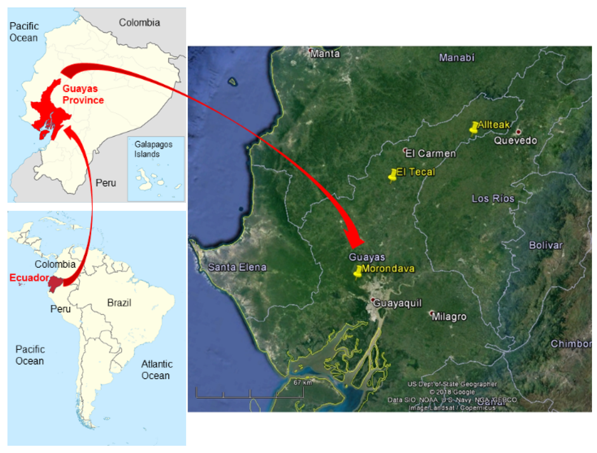
2.1. Study Area
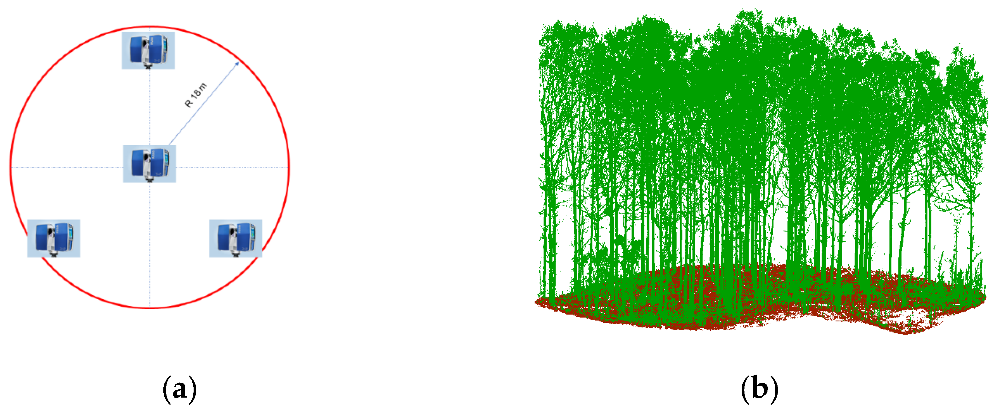
2.2. Field Data
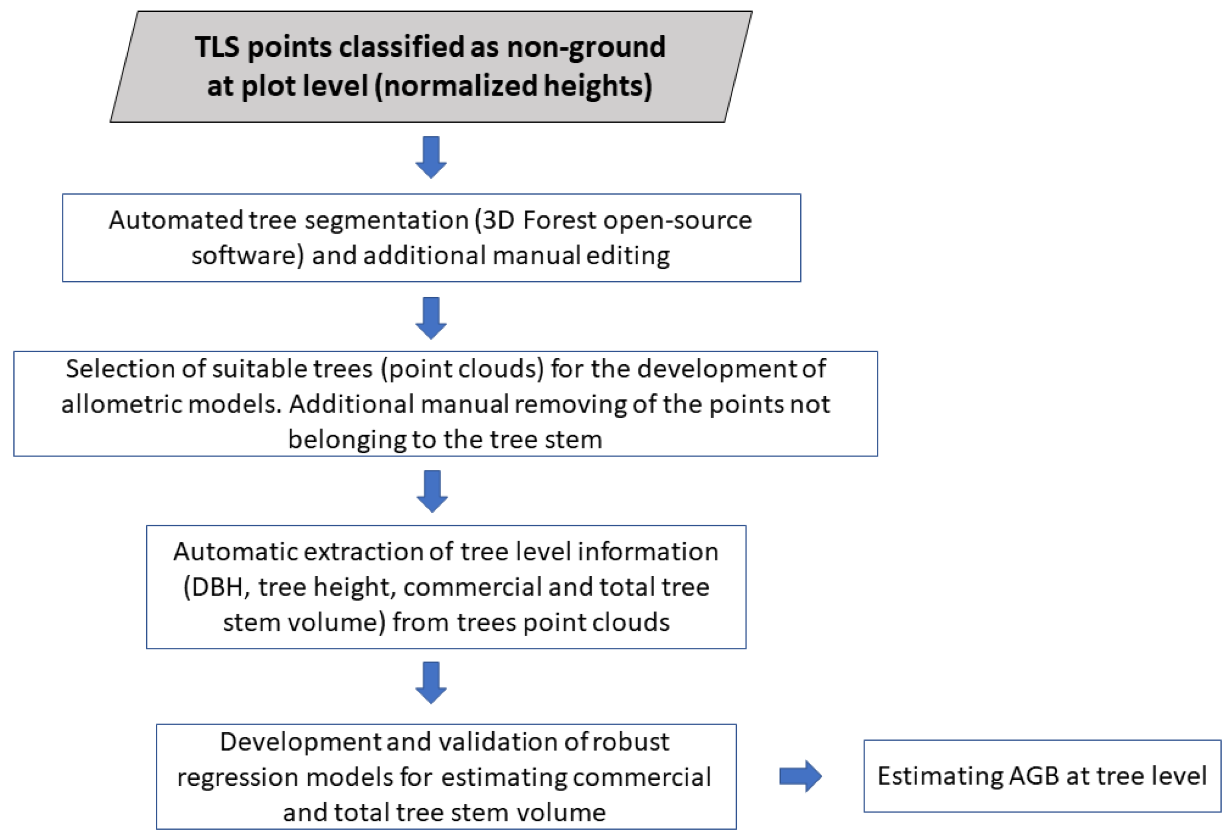
2.3. Tree Database Collection
2.3.1. Automated Tree Segmentation
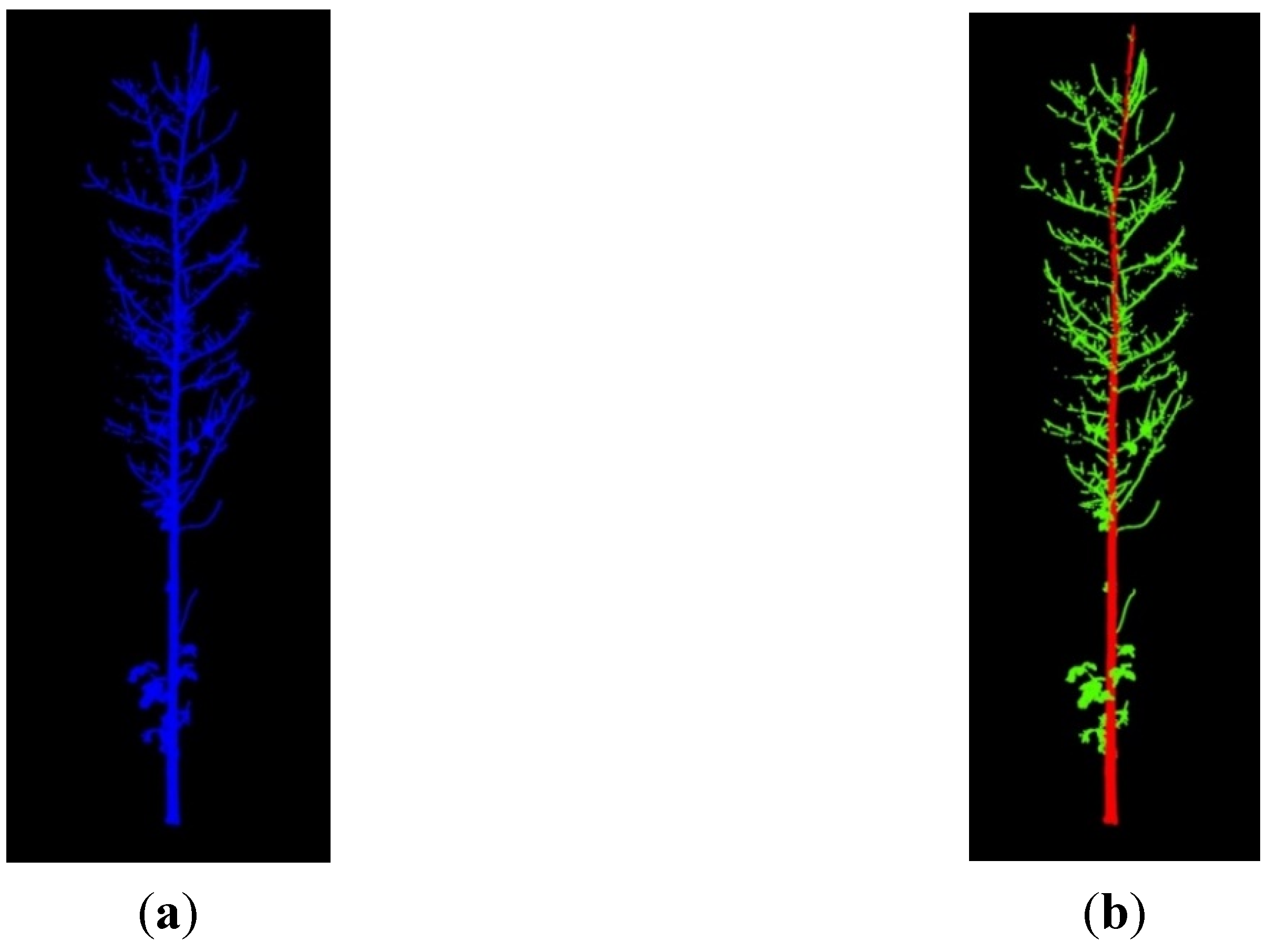
2.3.2. Selection of Suitable Trees
2.4. Automatic Extraction of Tree Level Information
2.5. Development and Validation of Allometric Models
- Global fitting. The model parameters were computed from all available sample teak trees (2272 individuals).
- DBH-based fitting. The original sample of teak trees was grouped into three classes according to DBH ranges ((5, 10), (10, 20), and (20, 30) cm). Therefore, three groups of model parameters were adjusted, one for each DBH range.
3. Results
3.1. Relationship Between DBH and Total Tree Height
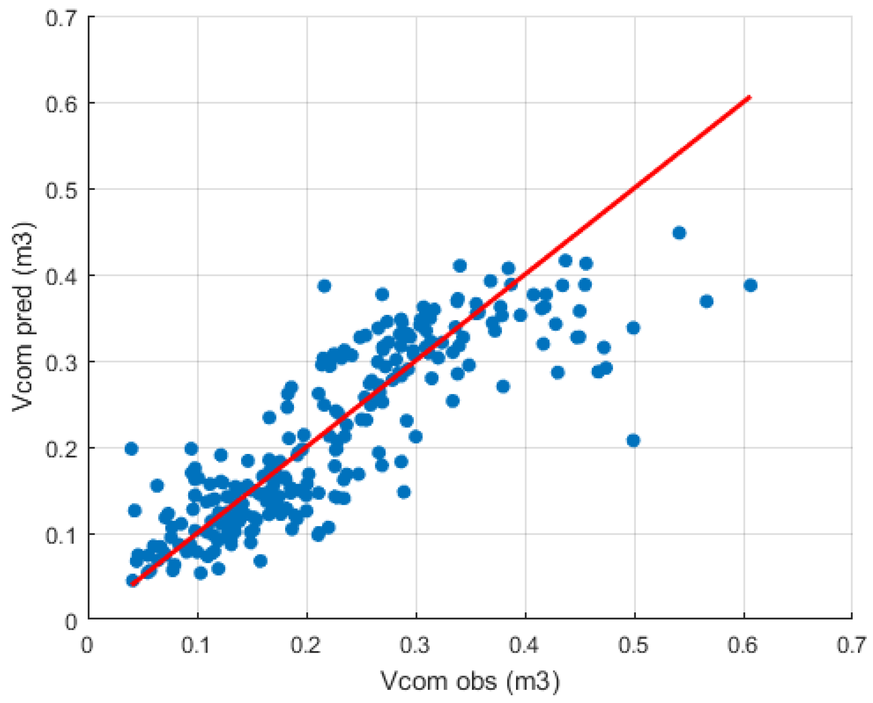
3.2. Allometric Model to Estimate Tree Commercial Volume
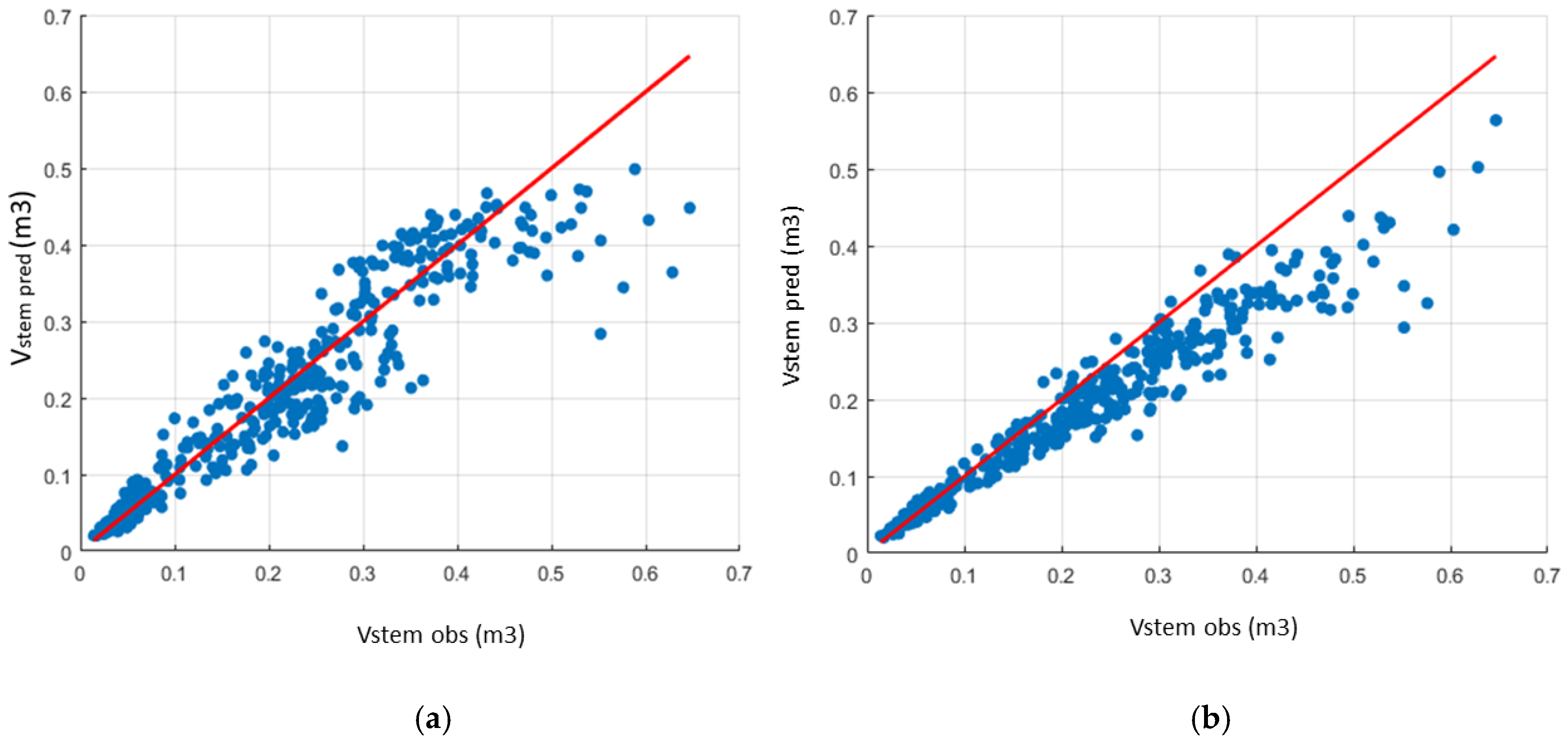
3.3. Allometric Model to Estimate Tree Stem Volume and Dry Biomass
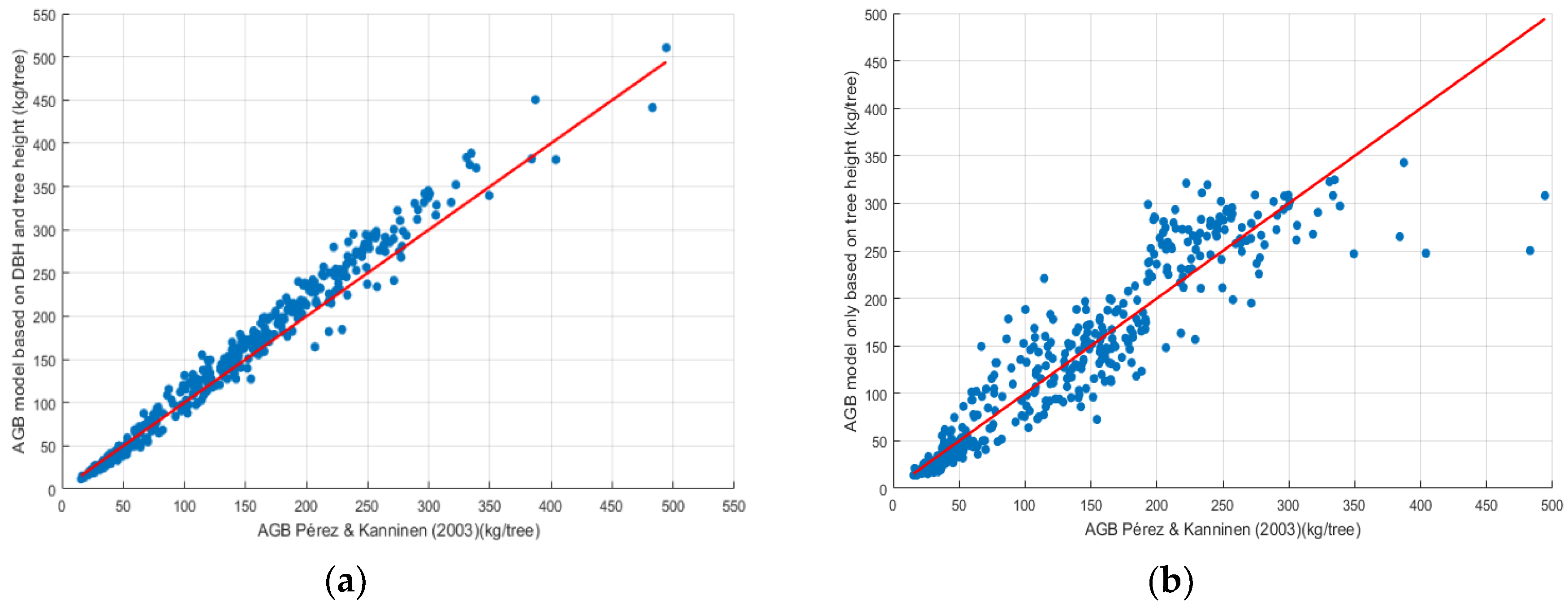
3.4. Allometric Model to Estimate the Above-Ground Biomass at Tree Level
- If we have the DBH and h of each tree:
- If we only have the tree height:Equation (15) would be applied, but substituting DBH for its estimation from the following expressions (see the DBH-based fitting model parameters in Table 2):
3.5. Descriptive Statistics of Some Dendrometric Variables
4. Discussion
5. Conclusions
Author Contributions
Funding
Acknowledgments
Conflicts of Interest
References
- Kollert, W.; Kleine, M. (Eds.) The Global Teak Study: Analysis, Evaluation and Future Potential of Teak Resources; IUFRO World Series Volume 36: Vienna, Austria, 2017; ISBN 978-3-902762-77-1. [Google Scholar]
- Food and Agriculture Organization of the United Nations. The State of the World’s Forest Genetic Resources; FAO of the United Nations: Rome, Italy, 2014. [Google Scholar]
- Kollert, W.; Cherubini, L. Teak Resources and Market. Assessment 2010; Planted Forests and Trees Working Paper FP/47/E; FAO of the United Nations: Rome, Italy, 2012. [Google Scholar]
- Midgley, S.; Somaiya, R.T.; Stevens, P.R.; Brown, A.; Nguyen, D.K.; Laity, R. Planted Teak: Global Production and Markets, with Reference to Solomon Islands; Technical Report 85; Australian Center for International Agricultural Research: Canberra, Australia, 2015.
- Cañadas, Á.; Andrade-Candell, J.; Domínguez, J.M.; Molina, C.; Schnabel, O.; Vargas-Hernández, J.J.; Wehenkel, C. Growth and Yield Models for Teak Planted as Living Fences in Coastal Ecuador. Forests 2018, 9, 55. [Google Scholar] [CrossRef]
- Kollert, W.; Przemyslaw, J.W. (Eds.) World Teak Resources, Production, Markets and Trade. In The Global Teak Study. Analysis, Evaluation and Future Potential of Teak Resources; IUFRO World Series Volume 36: Vienna, Austria, 2017; pp. 83–89. ISBN 978-3-902762-77-1. [Google Scholar]
- Agrawal, A.; Nepstad, D.; Chhatre, A. Reducing Emissions from Deforestation and Forest Degradation. Annu. Rev. Environ. Resour. 2011, 36, 373–396. [Google Scholar] [CrossRef]
- Dixon, R.K.; Solomon, A.M.; Brown, S.; Houghton, R.A.; Trexier, M.C.; Wisniewski, J. Carbon pools and flux of global forest ecosystems. Science 1994, 263, 185–190. [Google Scholar] [CrossRef] [PubMed]
- Houghton, R.A.; Nassikas, A.A. Negative emissions from stopping deforestation and forest degradation, globally. Glob. Chang. Biol. 2018, 24, 350–359. [Google Scholar] [CrossRef] [PubMed]
- Herold, M.; Johns, T. Linking requirements with capabilities for deforestation monitoring in the context of the UNFCCC-REDD process. Environ. Res. Lett. 2007, 2, 1–7. [Google Scholar] [CrossRef]
- Gibbs, H.K.; Brown, S.; Niles, J.O.; Foley, J.A. Monitoring and estimating tropical forest carbon stocks: Making REDD a reality. Environ. Res. Lett. 2007, 2, 045023. [Google Scholar] [CrossRef]
- Ferraz, A.; Saatchi, S.; Mallet, C.; Meyer, V. Lidar detection of individual tree size in tropical forests. Remote Sens. Environ. 2016, 183, 318–333. [Google Scholar] [CrossRef]
- Chave, J.; Réjou-Méchain, M.; Búrquez, A.; Chidumayo, E.; Colgan, M.S.; Delitti, W.B.C.; Duque, A.; Eid, T.; Fearnside, P.M.; Goodman, R.C.; et al. Improved allometric models to estimate the aboveground biomass of tropical trees. Glob. Chang. Biol. 2014, 20, 3177–3190. [Google Scholar] [CrossRef]
- Jucker, T.; Caspersen, J.; Chave, J.; Antin, C.; Barbier, N.; Bongers, F.; Dalponte, M.; van Ewijk, K.Y.; Forrester, D.I.; Haeni, M.; et al. Allometric equations for integrating remote sensing imagery into forest monitoring programmes. Glob. Chang. Biol. 2017, 23, 177–190. [Google Scholar] [CrossRef]
- Wulder, M.A.; Franklin, S.E. (Eds.) Remote Sensing of Forest Environments, Concepts and Case Studies, 1st ed.; Kluwer Academic Publishers: Boston, MA, USA, 2003; ISBN 978-1-4020-7405-9. [Google Scholar]
- White, J.C.; Coops, N.C.; Wulder, M.A.; Vastaranta, M.; Hilker, T.; Tompalski, P. Remote Sensing Technologies for Enhancing Forest Inventories: A Review. Can. J. Remote Sens. 2016, 42, 619–641. [Google Scholar] [CrossRef]
- Giannetti, F.; Puletti, N.; Quatrini, V.; Travaglini, D.; Bottalico, F.; Corona, P.; Chirici, G. Integrating terrestrial and airborne laser scanning for the assessment of single-tree attributes in Mediterranean forest stands. Eur. J. Remote Sens. 2018, 51, 795–807. [Google Scholar] [CrossRef]
- Suraj Reddy, R.; Rakesh, A.; Jha, C.S.; Rajan, K.S. Automatic Estimation of Tree Stem Attributes Using Terrestrial Laser Scanning in Central Indian Dry Deciduous Forests. Curr. Sci. 2018, 114, 201–206. [Google Scholar] [CrossRef]
- Liang, X.; Kankare, V.; Hyyppä, J.; Wang, Y.; Kukko, A.; Haggrén, H.; Yu, X.; Kaartinen, H.; Jaakkola, A.; Guan, F.; et al. Terrestrial laser scanning in forest inventories. ISPRS J. Photogramm. Remote Sens. 2016, 115, 63–77. [Google Scholar] [CrossRef]
- Du, S.; Lindenbergh, R.; Ledoux, H.; Stoter, J.; Nan, L. AdTree: Accurate, Detailed, and Automatic Modelling of Laser-Scanned Trees. Remote Sens. 2019, 11, 2074. [Google Scholar] [CrossRef]
- Saarinen, N.; Kankare, V.; Vastaranta, M.; Luoma, V.; Pyörälä, J.; Tanhuanpää, T.; Liang, X.; Kaartinen, H.; Kukko, A.; Jaakkola, A.; et al. Feasibility of Terrestrial laser scanning for collecting stem volume information from single trees. ISPRS J. Photogramm. Remote Sens. 2017, 123, 140–158. [Google Scholar] [CrossRef]
- Maas, H.-G.; Bienert, A.; Scheller, S.; Keane, E. Automatic forest inventory parameter determination from terrestrial laser scanner data. Int. J. Remote Sens. 2008, 29, 1579–1593. [Google Scholar] [CrossRef]
- Dassot, M.; Constant, T.; Fournier, M. The use of terrestrial LiDAR technology in forest science: Application fields, benefits and challenges. Ann. For. Sci. 2011, 68, 959–974. [Google Scholar] [CrossRef]
- Liang, X.; Kankare, V.; Yu, X.; Hyyppä, J.; Holopainen, M. Automated Stem Curve Measurement Using Terrestrial Laser Scanning. IEEE Trans. Geosci. Remote Sens. 2014, 52, 1739–1748. [Google Scholar] [CrossRef]
- Holopainen, M.; Vastaranta, M.; Kankare, V.; Räty, M.; Vaaja, M.; Liang, X.; Yu, X.; Hyyppä, J.; Hyyppä, H.; Viitala, R.; et al. Biomass estimation of individual trees using stem and crown diameter TLS measurements. ISPRS Int. Arch. Photogramm. Remote Sens. Spat. Inf. Sci. 2012, XXXVIII-5/W12, 91–95. [Google Scholar] [CrossRef]
- Kankare, V.; Holopainen, M.; Vastaranta, M.; Puttonen, E.; Yu, X.; Hyyppä, J.; Vaaja, M.; Hyyppä, H.; Alho, P. Individual tree biomass estimation using terrestrial laser scanning. ISPRS J. Photogramm. Remote Sens. 2013, 75, 64–75. [Google Scholar] [CrossRef]
- Calders, K.; Newnham, G.; Burt, A.; Murphy, S.; Raumonen, P.; Herold, M.; Culvenor, D.; Avitabile, V.; Disney, M.; Armston, J.; et al. Nondestructive estimates of above-ground biomass using terrestrial laser scanning. Methods Ecol. Evol. 2015, 6, 198–208. [Google Scholar] [CrossRef]
- Lau, A.; Calders, K.; Bartholomeus, H.; Martius, C.; Raumonen, P.; Herold, M.; Vicari, M.; Sukhdeo, H.; Singh, J.; Goodman, R. Tree Biomass Equations from Terrestrial LiDAR: A Case Study in Guyana. Forests 2019, 10, 527. [Google Scholar] [CrossRef]
- Raumonen, P.; Kaasalainen, M.; Åkerblom, M.; Kaasalainen, S.; Kaartinen, H.; Vastaranta, M.; Holopainen, M.; Disney, M.; Lewis, P. Fast Automatic Precision Tree Models from Terrestrial Laser Scanner Data. Remote Sens. 2013, 5, 491–520. [Google Scholar] [CrossRef]
- Lau, A.; Bentley, L.P.; Martius, C.; Shenkin, A.; Bartholomeus, H.; Raumonen, P.; Malhi, Y.; Jackson, T.; Herold, M. Quantifying branch architecture of tropical trees using terrestrial LiDAR and 3D modelling. Trees 2018, 32, 1219–1231. [Google Scholar] [CrossRef]
- Hackenberg, J.; Spiecker, H.; Calders, K.; Disney, M.; Raumonen, P. SimpleTree—An Efficient Open Source Tool to Build Tree Models from TLS Clouds. Forests 2015, 6, 4245–4294. [Google Scholar] [CrossRef]
- Delagrange, S.; Jauvin, C.; Rochon, P. PypeTree: A Tool for Reconstructing Tree Perennial Tissues from Point Clouds. Sensors 2014, 14, 4271–4289. [Google Scholar] [CrossRef]
- Gonzalez de Tanago, J.; Lau, A.; Bartholomeus, H.; Herold, M.; Avitabile, V.; Raumonen, P.; Martius, C.; Goodman, R.C.; Disney, M.; Manuri, S.; et al. Estimation of above-ground biomass of large tropical trees with terrestrial LiDAR. Methods Ecol. Evol. 2018, 9, 223–234. [Google Scholar] [CrossRef]
- Aguilar, F.J.; Rivas, J.R.; Nemmaoui, A.; Peñalver, A.; Aguilar, M.A.; Aguilar, F.J.; Rivas, J.R.; Nemmaoui, A.; Peñalver, A.; Aguilar, M.A. UAV-Based Digital Terrain Model Generation under Leaf-Off Conditions to Support Teak Plantations Inventories in Tropical Dry Forests. A Case of the Coastal Region of Ecuador. Sensors 2019, 19, 1934. [Google Scholar] [CrossRef]
- Flores Velasteguí, T.; Cabezas Guerrero, F.; Crespo Gutiérrez, R. Plagas y enfermedades en plantaciones de Teca (Tectona grandis L.F.) en la zona de Balzar, provincia de Guayas. Cienc. Tecnol. 2010, 3, 15–22. [Google Scholar] [CrossRef]
- Holdridge, L.R. Ecología Basada en Zonas de Vida; Instituto Interamericano de Cooperacion para la Agricultura: San José, Costa Rica, 1982; ISBN 9789290390398. [Google Scholar]
- Puletti, N.; Grotti, M.; Scotti, R. Evaluating the eccentricities of poplar stem profiles with terrestrial laser scanning. Forests 2019, 10, 239. [Google Scholar] [CrossRef]
- Chen, Q.; Gong, P.; Baldocchi, D.; Tian, Y.Q. Estimating Basal Area and Stem Volume for Individual Trees from Lidar Data. Photogramm. Eng. Remote Sens. 2007, 73, 1355–1365. [Google Scholar] [CrossRef]
- Tran-Ha, M.; Cordonnier, T.; Vallet, P.; Lombart, T. Estimation du volume total aérien des peuplements forestiers à partir de la surface terrière et de la hauteur de Lorey. Rev. For. Fr. 2011, 63, 361–378. [Google Scholar] [CrossRef][Green Version]
- Pueschel, P.; Newnham, G.; Rock, G.; Udelhoven, T.; Werner, W.; Hill, J. The influence of scan mode and circle fitting on tree stem detection, stem diameter and volume extraction from terrestrial laser scans. ISPRS J. Photogramm. Remote Sens. 2013, 77, 44–56. [Google Scholar] [CrossRef]
- Trochta, J.; Krůček, M.; Vrška, T.; Král, K. 3D Forest: An application for descriptions of three-dimensional forest structures using terrestrial LiDAR. PLoS ONE 2017, 12, e0176871. [Google Scholar] [CrossRef]
- Tao, S.; Wu, F.; Guo, Q.; Wang, Y.; Li, W.; Xue, B.; Hu, X.; Li, P.; Tian, D.; Li, C.; et al. Segmenting tree crowns from terrestrial and mobile LiDAR data by exploring ecological theories. ISPRS J. Photogramm. Remote Sens. 2015, 110, 66–76. [Google Scholar] [CrossRef]
- Zhang, W.; Wan, P.; Wang, T.; Cai, S.; Chen, Y.; Jin, X.; Yan, G. A novel approach for the detection of standing tree stems from plot-level terrestrial laser scanning data. Remote Sens. 2019, 11, 211. [Google Scholar] [CrossRef]
- Ladrón de Guevara, I.; Muñoz, J.; de Cózar, O.D.; Blázquez, E.B. Robust Fitting of Circle Arcs. J. Math. Imaging Vis. 2011, 40, 147–161. [Google Scholar] [CrossRef]
- Telles, R.; Gómez, M.; Alanís, E.; Aguirre, O.A.; Jiménez, J. Ajuste y selección de modelos matemáticos para predecir el volumen total fustal de Tectona grandis en Nuevo Urecho, Michoacán, México. Madera Bosques 2018, 24, e2431544. [Google Scholar]
- Bermejo, I.; Cañellas, I.; Miguel, A.S. Growth and yield models for teak plantations in Costa Rica. For. Ecol. Manag. 2004, 189, 97–110. [Google Scholar] [CrossRef]
- Armijos Guzmán, D.D. Construcción de Tablas Volumétricas y Cálculo del Factor de Forma para dos Especies, Teca (Tectona Grandis) y Melina (Gmelina arborea), en Tres Plantaciones de la Empresa Reybanpac C.A. en la Provincia de Los Ríos. Ph.D. Thesis, Escuela Superior Politécnica de Chimborazo, Escuela de Ingeniería Forestal, Cartago, Costa Rica, 2013. [Google Scholar]
- Ounban, W.; Puangchit, L.; Diloksumpun, S. Development of general biomass allometric equations for Tectona grandis Linn.F. and Eucalyptus camaldulensis Dehnh. plantations in Thailand. Agric. Nat. Resour. 2016, 50, 48–53. [Google Scholar] [CrossRef]
- Pérez, L.D.; Kanninen, M. Aboveground biomass of Tectona grandis plantations in Costa Rica. J. Trop. For. Sci. 2003, 15, 199–213. [Google Scholar]
- Dumouchel, W.; O’Brien, F. Integrating a robust option into a multiple regression computing environment. Inst. Math. Its Appl. 1991, 36, 41. [Google Scholar]
- Street, J.O.; Carroll, R.J.; Ruppert, D. A Note on Computing Robust Regression Estimates Via Iteratively Reweighted Least Squares. Am. Stat. 1988, 42, 152. [Google Scholar]
- Baskerville, G.L. Use of Logarithmic Regression in the Estimation of Plant Biomass. Can. J. For. Res. 1972, 2, 49–53. [Google Scholar] [CrossRef]
- Sumida, A.; Miyaura, T.; Torii, H. Relationships of tree height and diameter at breast height revisited: Analyses of stem growth using 20-year data of an even-aged Chamaecyparis obtusa stand. Tree Physiol. 2013, 33, 106–118. [Google Scholar] [CrossRef] [PubMed]
- Iizuka, K.; Yonehara, T.; Itoh, M.; Kosugi, Y.; Iizuka, K.; Yonehara, T.; Itoh, M.; Kosugi, Y. Estimating Tree Height and Diameter at Breast Height (DBH) from Digital Surface Models and Orthophotos Obtained with an Unmanned Aerial System for a Japanese Cypress (Chamaecyparis obtusa) Forest. Remote Sens. 2017, 10, 13. [Google Scholar] [CrossRef]
- West, G.B.; Brown, J.H.; Enquist, B.J. A general model for the structure and allometry of plant vascular systems. Nature 1999, 400, 664–667. [Google Scholar] [CrossRef]
- Huber, P.J.; Ronchetti, E.M. Robust Statistics, 2nd ed.; John Wiley & Sons: Hoboken, NJ, USA, 2009; ISBN 0470129905. [Google Scholar]
- Rousseeuw, P.J.; Croux, C. Alternatives to the Median Absolute Deviation. J. Am. Stat. Assoc. 1993, 88, 1273–1283. [Google Scholar] [CrossRef]
- White, J.C.; Tompalski, P.; Coops, N.C.; Wulder, M.A. Comparison of airborne laser scanning and digital stereo imagery for characterizing forest canopy gaps in coastal temperate rainforests. Remote Sens. Environ. 2018, 208, 1–14. [Google Scholar] [CrossRef]
- Lara, C.E. Aplicación de ecuaciones de conicidad para teca (Tectona grandis L.F.) en la zona costera ecuatoriana. Cienc. Tecnol. 2012, 4, 19–27. [Google Scholar] [CrossRef]
- Crespo, R.; Jiménez, E.; Suatunce, P.; Law, G.; Sánchez, C. Análisis comparativo de las propiedades físico-mecánicas de la madera de teca (Tectona grandis L.F.) de Quevedo y Balzar. Cienc. Tecnol. 2008, 1, 55–63. [Google Scholar] [CrossRef]
- Flórez, J.B.; Trugilho, P.F.; Lima, J.T.; Hein, P.R.G.; Silva, J.R.M. da Characterization of young wood Tectona grandis L. F. planted in Brazil. Madera Bosques 2014, 20, 11–20. [Google Scholar]
- Valero, S.W.; Reyes, E.C.; Garay, D.A. Estudio de las propiedades físico-mecánicas de la especie Tectona grandis, de 20 años de edad, proveniente de las plantaciones de la Unidad Experimental de la Reserva Forestal Ticoporo, Estado Barinas. Rev. For. Venez. 2005, 49, 61–73. [Google Scholar]
- Rivero, J.; Moya, R. Propiedades físico-mecánicas de la madera de Tectona grandis Linn. F. (teca), proveniente de una plantación de ocho años de edad en Cochabamba, Bolivia. Kurú Rev. For. 2006, 3, 1–14. [Google Scholar]
- Pérez, L.D.; Kanninen, M. Heartwood, sapwood and bark content, and wood dry density of young and mature teak (Tectona grandis) trees grown in Costa Rica. Silva. Fenn. 2003, 37, 45–54. [Google Scholar]
- Krishnapillay, D.B. Silviculture and management of teak plantations. Unasylva 2000, 51, 14–21. [Google Scholar]
- Mora, F.; Hernández, W. Estimación del volumen comercial por producto para rodales de teca en el Pacífico de Costa Rica. Agron. Costarric. 2007, 31, 101–112. [Google Scholar]
- Ota, T.; Ogawa, M.; Shimizu, K.; Kajisa, T.; Mizoue, N.; Yoshida, S.; Takao, G.; Hirata, Y.; Furuya, N.; Sano, T.; et al. Aboveground Biomass Estimation Using Structure from Motion Approach with Aerial Photographs in a Seasonal Tropical Forest. Forests 2015, 6, 3882–3898. [Google Scholar] [CrossRef]
- Guerra-Hernández, J.; González-Ferreiro, E.; Monleón, V.; Faias, S.; Tomé, M.; Díaz-Varela, R. Use of Multi-Temporal UAV-Derived Imagery for Estimating Individual Tree Growth in Pinus pinea Stands. Forests 2017, 8, 300. [Google Scholar] [CrossRef]
- Popescu, S.C.; Wynne, R.H. Seeing the Trees in the Forest. Photogramm. Eng. Remote Sens. 2004, 70, 589–604. [Google Scholar] [CrossRef]
- Feldpausch, T.R.; Lloyd, J.; Lewis, S.L.; Brienen, R.J.W.; Gloor, M.; Monteagudo Mendoza, A.; Lopez-Gonzalez, G.; Banin, L.; Abu Salim, K.; Affum-Baffoe, K.; et al. Tree height integrated into pantropical forest biomass estimates. Biogeosciences 2012, 9, 3381–3403. [Google Scholar] [CrossRef]
- Iida, Y.; Kohyama, T.S.; Kubo, T.; Kassim, A.R.; Poorter, L.; Sterck, F.; Potts, M.D. Tree architecture and life-history strategies across 200 co-occurring tropical tree species. Funct. Ecol. 2011, 25, 1260–1268. [Google Scholar] [CrossRef]
- Hemery, G.E.; Savill, P.S.; Pryor, S.N. Applications of the crown diameter–stem diameter relationship for different species of broadleaved trees. For. Ecol. Manage. 2005, 215, 285–294. [Google Scholar] [CrossRef]
- Spicer, R.; Groover, A. Evolution of development of vascular cambia and secondary growth. New Phytol. 2010, 186, 577–592. [Google Scholar] [CrossRef] [PubMed]
- Shinozaki, K.; Yoda, K.; Hozumi, K.; Kira, T. A quantitative analysis of plant form. The pipe model theory: I. Basic analyses. Jpn. J. Ecol. 1964, 14, 97–105. [Google Scholar]


| Class | DBH (cm) | Selected Trees |
|---|---|---|
| 1 | [5,10] | 100 |
| 2 | (10,15] | 100 |
| 3 | (15,20] | 146 |
| 4 | (20,25] | 100 |
| 5 | > 25 | 10 |
| Total | 456 |
| Statistics | Global Fitting 2272 Trees | DBH-Based Fitting 5 ≤ DBH (cm) < 10 958 Trees | DBH-Based Fitting 10 ≤ DBH (cm) < 20 1110 Trees | DBH-Based Fitting 20 ≤ DBH (cm) < 30 204 Trees |
|---|---|---|---|---|
| RMSE (cm) | 1.69 (0.10) | 0.88 (0.07) | 1.53 (0.13) | 1.46 (0.10) |
| Relative RMSE (%) | 13.85 | 10.65 | 11.10 | 6.65 |
| Bias (%) | 1.32 (0.81) | 1.97 (1.03) | 0.81 (0.99) | 0.15 (0.62) |
| σ | 0.1778 | 0.1167 | 0.1094 | 0.0685 |
| α (p < 0.001) | 0.1055 | 0.8904 | 0.5605 | 2.1430 |
| β (p < 0.001) | 0.9580 | 0.5696 | 0.7863 | 0.3148 |
| Kind of Fitting Model | DBH Class * | RMSE (kg/tree) | Relative RMSE (%) | Bias (%) |
|---|---|---|---|---|
| Global fitting model | class 1 | 12.06 | 47.63 | 23.24 |
| class 2 | 26.43 | 29.61 | 4.85 | |
| class 3 | 71.14 | 28.55 | −19.84 | |
| DBH-based fitting model ** | class 1 | 6.19 | 24.47 | 5.19 |
| class 2 | 24.69 | 27.67 | 3.49 | |
| class 3 | 45.28 | 18.17 | −0.62 |
| Allometric Model | RMSE (m3) | Relative RMSE (%) | Bias (%) |
|---|---|---|---|
| 0.0574 | 25.74 | 11.27 | |
| 0.0741 | 33.22 | 12.72 | |
| 0.0482 | 21.60 | 8.64 | |
| * | 0.0608 | 27.24 | 1.43 |
| Allometric Model | RMSE (m3) | Relative RMSE (%) | Bias (%) |
|---|---|---|---|
| 0.0413 | 21.25 | 1.03 | |
| 0.0503 | 25.88 | 2.54 | |
| 0.0319 | 16.41 | 0.37 | |
| * | 0.0461 | 23.72 | −1.11 |
| DBH Class | Tree Stem Commercial Volume (m3) | Tree Stem Dry Biomass (kg/tree) | AGB (kg/tree) |
|---|---|---|---|
| 5–10 cm | 20.52 (4.74) | 25.65 (5.93) | |
| 10–15 cm | 42.08 (18.57) | 52.60 (23.22) | |
| 15–20 cm | 0.1483 (0.056) | 125.98 (28.43) | 157.48 (35.54) |
| 20–25 cm | 0.3036 (0.075) | 205.46 (39.58) | 256.82 (49.47) |
| 25–30 cm | 0.4885 (0.061) | 302 (37.60) | 378.45 (47.01) |
© 2019 by the authors. Licensee MDPI, Basel, Switzerland. This article is an open access article distributed under the terms and conditions of the Creative Commons Attribution (CC BY) license (http://creativecommons.org/licenses/by/4.0/).
Share and Cite
Aguilar, F.J.; Nemmaoui, A.; Peñalver, A.; Rivas, J.R.; Aguilar, M.A. Developing Allometric Equations for Teak Plantations Located in the Coastal Region of Ecuador from Terrestrial Laser Scanning Data. Forests 2019, 10, 1050. https://doi.org/10.3390/f10121050
Aguilar FJ, Nemmaoui A, Peñalver A, Rivas JR, Aguilar MA. Developing Allometric Equations for Teak Plantations Located in the Coastal Region of Ecuador from Terrestrial Laser Scanning Data. Forests. 2019; 10(12):1050. https://doi.org/10.3390/f10121050
Chicago/Turabian StyleAguilar, Fernando J., Abderrahim Nemmaoui, Alberto Peñalver, José R. Rivas, and Manuel A. Aguilar. 2019. "Developing Allometric Equations for Teak Plantations Located in the Coastal Region of Ecuador from Terrestrial Laser Scanning Data" Forests 10, no. 12: 1050. https://doi.org/10.3390/f10121050
APA StyleAguilar, F. J., Nemmaoui, A., Peñalver, A., Rivas, J. R., & Aguilar, M. A. (2019). Developing Allometric Equations for Teak Plantations Located in the Coastal Region of Ecuador from Terrestrial Laser Scanning Data. Forests, 10(12), 1050. https://doi.org/10.3390/f10121050