Article

Understanding the Critical Impact Path on Vegetation Growth under Climate Extremes and Human Influence

1
Korea Adaptation Center for Climate Change, Korea Environment Institute, Sejong 30147, Korea
2
Graduate School of Environmental Studies, Seoul National University, Seoul 08826, Korea
3
Department of Landscape Architecture and Rural System Engineering, CALS, Seoul National University, Seoul 08826, Korea
*
Author to whom correspondence should be addressed.
Forests 2019, 10(11), 947; https://doi.org/10.3390/f10110947
Submission received: 2 September 2019 / Revised: 13 October 2019 / Accepted: 23 October 2019 / Published: 24 October 2019
(This article belongs to the Section Forest Ecology and Management)

Abstract

:
Reduced vegetation growth ultimately induces degradation of the ecosystem and CO2 sequestration. Multiple risks can affect vegetation, but climate change and human influence have been particularly known to be major risks for deteriorating the ecosystem. However, there is limited information illustrating comprehensive impact pathways that consider both climatic and human impacts on vegetation. To promote optimum decision-making, information is required to elucidate complex cause-and-effect pathways in order to determine how various impacts are related and which ones are more important. Hence, we identified impact pathways affecting enhanced vegetation index (EVI) regarding climate and human factors by revealing a causal network using the Bayesian network approach. Vulnerable vegetation types and the spatial range of impact were evaluated based on the identified network by analyzing temporal changes in annual average EVI, human-induced land conversion, and multiple climate extremes from 2002 to 2014 on Jeju Island, South Korea. The results indicated the high vulnerability of coniferous forests compared with mixed and deciduous forests were able to elucidate the major impact paths, including human-induced land conversion at lower elevation, length of frost, degree of heat, and general intensity of wetness (Pearson’s r = 0.58). Existing policies in the study site have been insufficient to avoid the major paths influencing vegetation state. This study offers insights into comprehensive impact paths in order to support effective decision-making for nature conservation.

Graphical Abstract

1. Introduction

Vegetation is a key component of an ecosystem; hence, sustaining vegetation health is a fundamental requirement to sustain the benefits of nature. A decrease in vegetation health alters the quantity and quality of ecosystem services, including decreases in biodiversity, carbon sequestration, and water conservation [1,2,3,4,5]. Generally, changes in vegetation health are triggered by climatic factors and human activities on regional and global scales [6,7,8,9]. In this respect, the convention of biological diversity has strongly emphasized the necessity of focusing on climatic and human influences for the management of ecosystems [10,11].
The impacts of climate factors and human activities on vegetation have been well studied. A recent assessment report by the IPCC (Intergovernmental Panel on Climate Change) concluded that a vegetation shift had occurred over the last decades due to global warming [12,13]. The IUCN (International Union for Conservation of Nature) has also listed newly threatened plant species in response to climate change [14]. As for the human impact on vegetation, biophysical and biogeochemical impacts caused by land conversion (LC) are definite and emphasize their negative influence on vegetation [15]. However, comprehensive assessments that consider both driving forces are limited [16], although several attempts have been made for Central Asia [9] and China, including the Loess plateau [8,17,18,19]. Therefore, there is a need to enhance our understanding of these two direct hazards in order to promote sustainable vegetation growth. As common failures in ecosystem management can arise from disagreements over the best decision [20,21,22], consideration of the two main risks may help reduce such disagreements.
However, it is challenging to consider both climate and human impacts on vegetation state (vegetation growth, coverage, and health). First of all, the characteristics of the two impacts that affect vegetation state can be different. As for the climate impact, rather than one single climate event, the occurrence of multiple climate extremes may cause a fatal response in vegetation [23,24], as there are various aspects of climate extremes (e.g., dryness, coldness) [25]. As such, one or multiple climate extremes can trigger large vegetation losses [25]. In the case of human activities, human-induced LC of natural vegetation is linked with unsustainable land management practices, which can quantitatively reduce or reverse such degradation [26]. Hence, depending on land management decisions, the size and degree of vegetation degradation can be different. Second, the response of vegetation can differ depending on the vegetation type (e.g., coniferous or deciduous) and elevation gradient [27,28]. Some vegetation types are vulnerable to climate change while others can respond positively, such as those used for firewood. Moreover, the occurrence of climate and human impacts can be particularly high at certain elevations.
In this respect, a systematic understanding of how these impacts occur and which impact is more important for each vegetation type or elevation is required. Specifically, as multiple factors exist and there can be various causalities and cascading relationships among each element, we need a clear understanding of such cause-and-effect paths in order to allocate finite management resources. However, it is challenging to identify such complex cause-and-effect relationships when considering multiple impacts. A regression equation cannot consider complex, layered interactions between multiple climate and human factors [17]. In this context, we applied a Bayesian network (BN) to elucidate the underlying causal network regarding multiple climate extremes and human-induced LC regarding vegetation state to systematically measure such causality. BNs are known for their strength in graphically illustrating various causalities and relative importance with directed acyclic graphs [29,30]. Machine learning techniques developed for BNs make it possible to automatically generate the underlying cause-and-effect network, which can indicate the major impacts and main causal sequences of such impacts [31].
Hence, in this study, we aimed to identify important driving forces and their critical impact pathway regarding vegetation state considering climate and human factors by quantifying a causal network using the BN approach to elucidate a prioritized management agenda. This study aimed to identify the differences in impact for vegetation state between climate and human factors, as well as to reveal vulnerable vegetation types and required management actions considering elevation gradients. To measure changes in the health and growth of vegetation, the enhanced vegetation index (EVI), a satellite-based vegetation greenness index, was used, since it is one of the most important data indices in ecosystems research and reflects the growth and status of surface vegetation [28]. To offer evidence-based information, we focused on changes in the annual average EVI and considered threatening factors from 2002 to 2015. In particular, we focused on Jeju Island in South Korea, where the whole area is designated as a UNESCO (United Nations Educational, Scientific and Cultural Organization) biosphere reserve due to its ecological importance.

2. Materials and Methods

2.1. Study Site and Vegetation for Case Study

The study site, Jeju Island (33.22° N, 126.32° E/33.37° N, 126.53° E), is located south of the Korean Peninsula. It is a volcanic island that contains unique biodiversity features and has various floristic elements, including temperate forests, arctic–alpine plants, and also deciduous and evergreen broad-leaved trees [32]. The island is unique as it overlaps four internationally designated areas (IDAs) due to its outstanding biological importance [33].
In this study site, three vegetation types were considered for analysis (Figure 1). That is, areas with a minimum of 75% coverage of vegetation for each coniferous, deciduous, and mixed tree species were evaluated based on the fifth forest type map of the Korea forest service (map.forest.go.kr). Vegetation located below 500 m above sea level was only considered to avoid vegetation located in high elevations, as a strictly protected area without any LC is located at upper elevations.
Random points were generated considering differences in age, density, and diameter based on the fifth forest type map (map.forest.go.kr). An equal number of random points were distributed regarding such factors using ArcGIS10.6. [34]. In total, 43,868 random points were considered. The numbers of random points for coniferous, deciduous, and mixed vegetation were 28,870, 8165, and 6833, respectively (Figure 1). The random points were later divided based on classified elevation, which were 0–200 m, 201–400 m, and 401–500 m, to elucidate differences in elevation gradient.

2.2. Data Processing for Annual Average EVI (EVIavg)

In this study, the EVI remote sensing vegetation index was used to evaluate vegetation states, as it reflects vegetation growth, coverage, and health [35,36]. EVI has been recognized to have less sensitivity to atmospheric effects than NDVI (Normalized Difference Vegetation Index) and can effectively capture canopy density beyond where NDVI becomes saturated [35,37].
To monitor vegetation states, EVI from 2002 to 2015 from the MODIS13A1.006 product was acquired through EARTHDATA NASA (earthdata.nasa.gov/). The MODIS13A1.006 product (500 m) was selected, as the previous version of EVI (Terra-C5 VIs) had lower product quality, particularly after 2007 [38]. Based on pixel reliability, only pixels of 0–1 with high reliability were selected, and the remaining low-quality pixels were masked for each satellite image. A Savitzky–Golay (SG) filter [39] was applied to fill the masked pixels and smooth the EVI to avoid biases, since it is known as a robust filter-based method to replace outliers, spikes, and missing values.
Specifically, every day of year (DOY) in the growing season from DOY81 to DOY289 which showed no snow in the study site was considered for analysis. Although Jeju Island has evergreen tree species, as it snows regularly in January and February (Korea meteorological administration, KMA, www.weather.go.kr), only DOYs in the growing season were considered. To consider temporal changes in EVI at the study site, this study quantified the annual average EVI values for each year (EVIavg) from 2002 to 2015. Hence, for each random point generated, 14 EVIavg values were acquired. We applied EVIavg because an average value can avoid further biases by representing a general vegetation state.

2.3. Data Processing for Land Conversion

As for LC, this study used the 500 m MODIS (Moderate Resolution Imaging Spectroradiometer) land cover product MCD12Q1. From 2001 to 2015, the MCD12Q1 was acquired through EARTHDATA NASA (earthdata.nasa.gov/). A land cover map based on international geosphere–biosphere programme (IGBP) classification was used in this study. Though we investigated the quality control (QC) layer to avoid classification errors, only LC from natural and planted vegetation to crop land, urban area, and barren land was considered. We note that such LC does not belong to illogical transitions, which are occasionally found in MCD12Q1 (see Peng et al. [40]). Accordingly, annual statistics on LC from natural and planted vegetation to crop land, urban area, and barren land were generated from 2001/2002 to 2014/2015 in each 500 m × 500 m grid. The quantification was conducted using Rstudio [41] applying the raster and rgdal packages.

2.4. Climate Extreme Indices

The team on climate change detection and indices (ETCCDI) developed a set of meteorological indices that represents regularly occurring climate extremes (see Zhang et al. [42]). Each index reflects cut tails on the distribution of precipitation or temperature. As it only considers “daily minimum temperature, maximum temperature, and precipitation”, mean temperature was excluded from the quantification process of such indices. Though the original ETCCDI indices do not include indices related to heat wave (HW) and heavy rain (HR) days, this study additionally considered HW and HR, as Jeju regularly has such climate extremes annually. Furthermore, to reflect the aspect of drought, this study also considered the annual average standardized precipitation–evapotranspiration index (SPEI)12 index from the global SPEI database based on Beguería et al. [43]. In summary, a total of eight climate extreme indices were considered (Table 1).
This study used 1 km × 1 km grid meteorological information acquired from the Korea meteorological administration (KMA, www.kma.go.kr). There are few meteorological stations in our study site, so we used modeled grid climate data based on the MK-prismv1.2. climate model developed by the KMA. To validate such grid information, we quantified and compared the climate extreme index with observed data using the R package climdex.pcic (http://cran.r-project.org/web/packages/climdex.pcic/). As the grid information has high reliability (Pearson’s r = 0.93, p < 0.001) with the observed climate (Figure S1), we used such information to reflect the multiple climate extremes indicated in Table 1.

2.5. Construction of Bayesian Network

A BN was applied to analyze the causal path between various climate extreme indices and human-induced LC regarding changes in EVIavg (Figure 2). In this study, a Gaussian BN was applied, which accounted for continuous variables with numeric values (BN for continuous values) [44]. To build an evidence-based network structure and its conditional path, we employed a learning-based BN by applying the bnlearn package using Rstudio. bnlearn supports the construction of a BN with several algorithms related to a conditional independence test and network scores measuring goodness of fit for structuring layered relationships [44]. Specifically, we first confirmed the appropriateness of the selected multiple variables (measured VIF (Variance Inflation Factor) < 6) [45] by identifying multicollinearity by performing a VIF test using the car package. To select a suitable algorithm to develop the BN, we also compared the accuracy of relevant algorithms. K-fold cross-validation (number of folds = 10) was performed for the entire sample dataset (n = 614,152), and the expected log-likelihood loss in structuring the optimal causal structure was quantified. Between the max-min hill-climbing (mmhc) and restricted maximization (rsmax2) algorithms, the performances were similar (expected loss = 9.20–9.21), but this study applied the mmhc algorithm (expected loss = 9.20) to construct the Gaussian BN. mmhc is an algorithm that constructs a skeleton of the BN with constraint-based and search-and-score techniques [46,47].
The Gaussian BN was made with several user-defined principles. The whitelisting function in bnlearn supports the logical structure by reflecting predefined linkages to avoid illogical linkage. Using the whitelisting function, this study whitelisted linkages from nine considered variables to EVIavg for understanding the magnitude of the impact that multiple driving forces have on EVIavg. The layered relationships between each factor were learned by an iteration process while finding the optimal network structure.
Specifically, the BN was generated per vegetation type (coniferous, mixed, and deciduous). The magnitude of impact per factor was measured from the generated Gaussian BN. To analyze the differences in impact for each elevation that reflected differences in EVI per elevation and spatial range of this impact, a Gaussian BN was additionally generated for 0–200 m, 201–400 m, and 401–500 m per vegetation type, separately.

2.6. Validation of Developed Bayesian Networks

To validate and investigate the accuracy of the BN, a dataset for each vegetation type was partitioned to train and test data with ratios of 0.75 and 0.25, which was conducted for all the random points considered. A BN was generated and fitted with training data (ratio = 0.75) for each vegetation type; thus, three BNs were first constructed. As for the second step, three test datasets (ratio = 0.25) for each BN were applied to the developed BN from the training dataset to quantify the predicted EVIavg values. Among the predicted and actual EVIavg in the test dataset, Pearson correlation analysis was performed to inspect the accuracy of the BNs.

3. Results

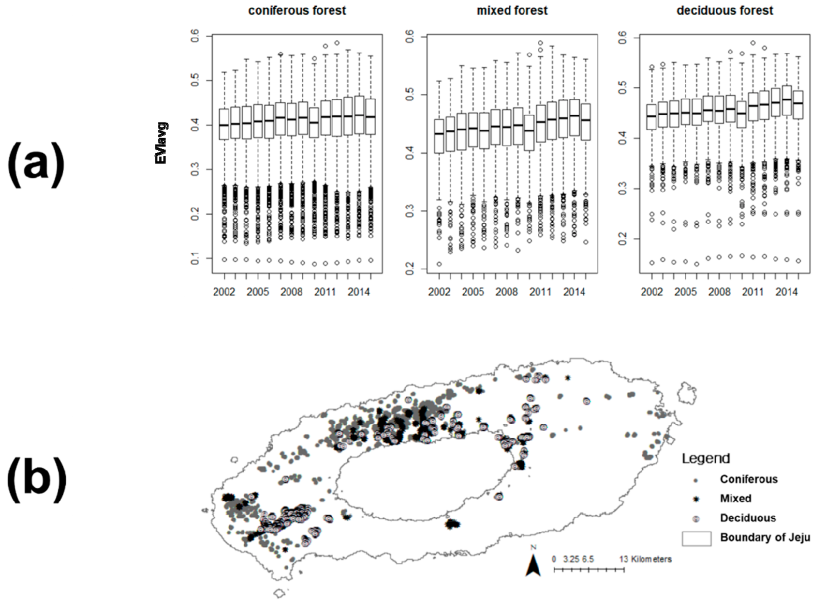
3.1. Temporal Changes in EVI

For the three vegetation types evaluated, the EVIavg tended to generally exhibit an increasing pattern from 2002 to 2015 (Figure 3). However, representative decreasing patterns in EVIavg were equally observed for 2009–2010 and 2014–2015 (Figure 3). Though the temporal pattern of EVIavg generally exhibited an ascending trend, for all random points considered, EVIavg was reduced in 2015 compared with EVIavg in 2002, showing a broad distribution pattern. This shows that there are certain widely distributed locations or time periods which have exhibited decreased EVI over a 14-year period. For all the evaluated points for coniferous, mixed, and deciduous forests, the percentages that showed a decreased EVIavg between 2002 and 2015 were 19%, 11%, and 12%, respectively (Figure 3).

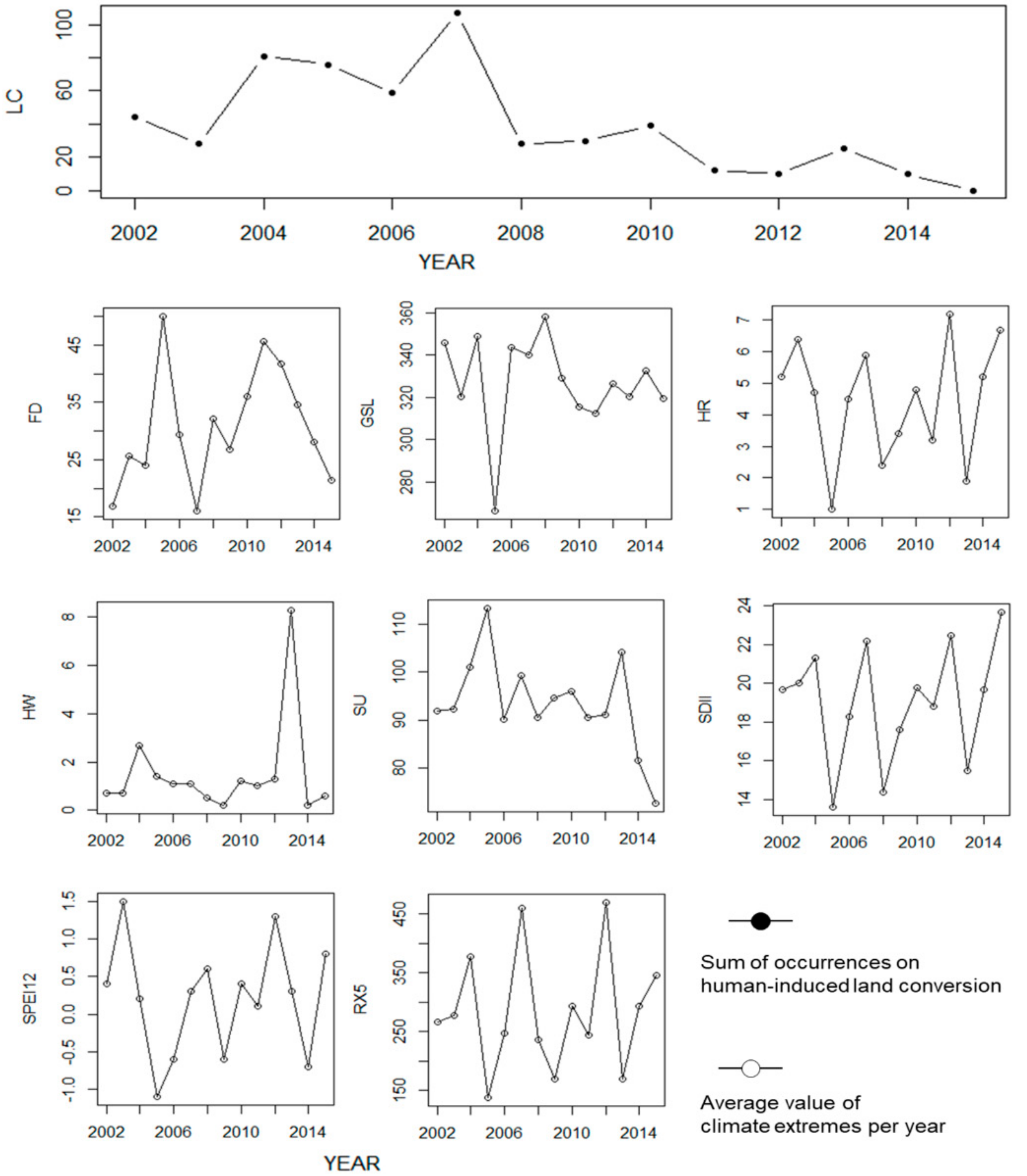
3.2. Temporal Changes in Human-Induced Land Conversion and Climate Extremes

Figure 4 shows the changes in the rate of human-induced LC and the occurrence of multiple climatic factors. For all 43,868 points considered, 1.22%, or 537 points, had experienced human-induced LC. As for 12 random points among all the locations considered, such human-induced land cover change occurred twice from 2002 to 2015. A significant increase in such human influence was observed in 2007 and 2004. However, the occurrences of human-induced LC showed a decreasing pattern overall (Figure 4).
In the meantime, each climate index had a distinct pattern in terms of annual average values. Rather than having clear decreasing or increasing trends, they had a zig-zag pattern but illustrated peak points. That is, the occurrence of climate extremes showed high variation from 2002 to 2015. Climate-related extremes for frost days (FD), growing season length (GSL), HW, and summer days (SU) exhibited wide variances. However, precipitation-related extremes, which were HR, maximum consecutive 5-day precipitation (RX5), simple daily intensity index (SDII), and SPEI12, showed more agreement than climate-related extremes.

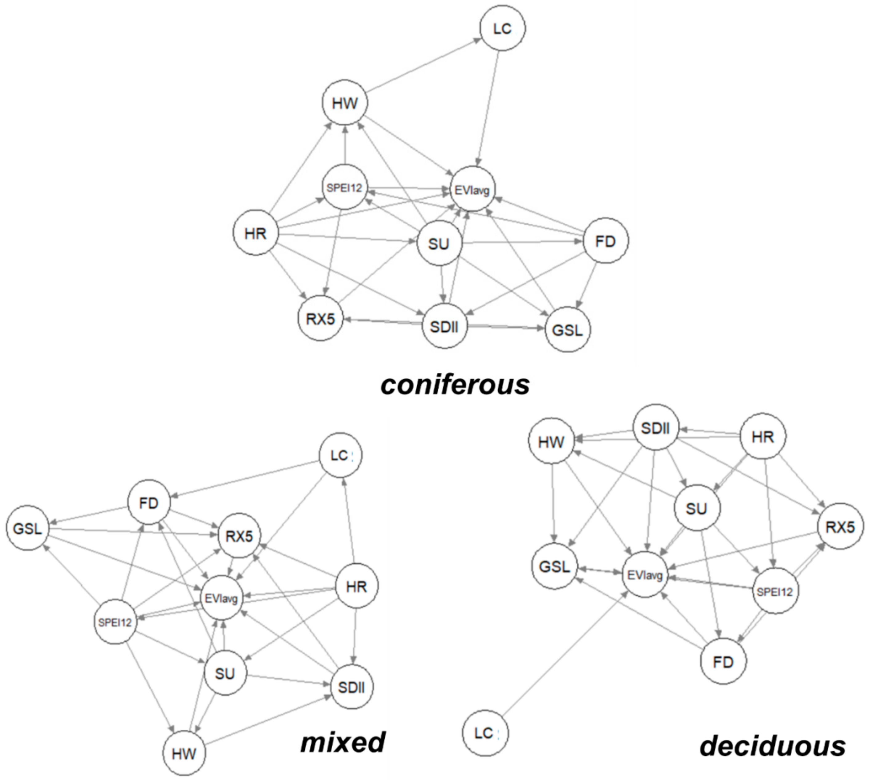
3.3. Causal Network among EVIavg, Climate Extremes, and Human-Induced Land Cover Change

3.3.1. Climate and Human Impacts per Vegetation Type

A BN was developed for each vegetation type regarding changes in EVIavg, rate of human-induced LC, and multiple climate extremes (Figure 5). The causal network showed that each vegetation type exhibited different causal relationships for the climate and human influence factors considered for vegetation states. The accuracy generated by the constituted BN showed relatively vulnerable vegetation types that were most affected by the driving forces considered. The accuracy was generated by comparing the predicted EVIavg from the BN developed and the actual EVIavg from the MODIS13A1.006 product in the test dataset. Coniferous forests were the most vulnerable vegetation type regarding the factors considered (Pearson’s r = 0.58). Mixed forests exhibited moderate accuracy within the driving forces considered (Pearson’s r = 0.34), whereas, in the case of deciduous forest, it showed the lowest correlation among predicted and actual EVIavg (Pearson’s r = 0.17). As a result, regarding climate and human impacts, coniferous forests were evaluated as the most influenced vegetation type, followed by mixed forests.
Table 2 shows the degree of relative influences on changes in EVIavg. Overall, the results showed that coniferous and mixed forests exhibited changes in EVIavg due to the combined effect of climatic and human factors rather than one particular factor. As for deciduous and mixed forests, the strong impact of human-induced LC was more distinct (conditional density = −0.53 and −0.34) than climatic factors.

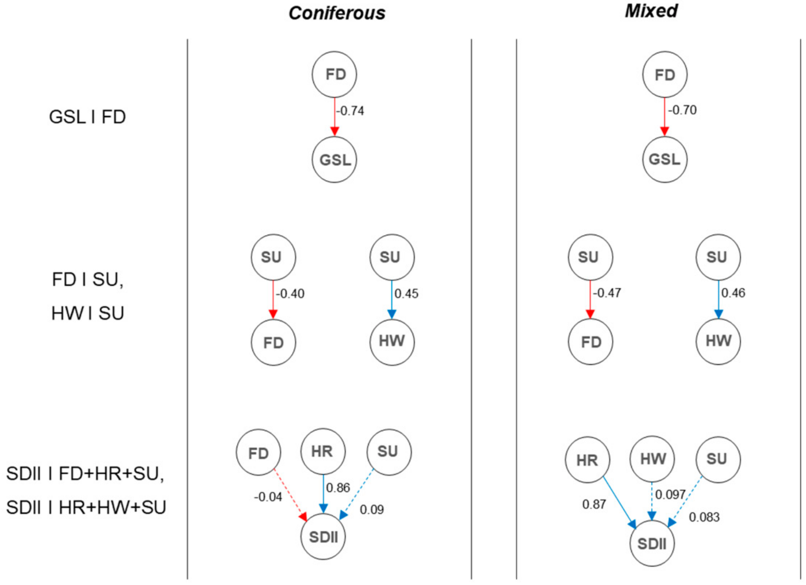
3.3.2. Critical Impact Path Regarding Human-Induced LC

Though the magnitude of impact regarding human-induced LC was different for the three vegetation types, it exhibited a consistently negative relationship with changes in EVIavg. Specifically, changes in land cover reduced the EVIavg for coniferous, mixed, and deciduous forests with a conditional density of −0.27, −0.34, and −0.53, respectively (Table 3). As for causal networks individually developed per level of elevation, it showed that a negative impact due to human-induced LC was particularly obvious at 0–200 m (Table 3). Only coniferous forests were affected by human-induced LC at 201–400 m. Overall, the results indicated that human-induced LC mainly influenced the vegetation state in lower areas (~200 m). Moreover, coniferous forests were affected by human-induced LC to a broader spatial extent than other vegetation types.
Meanwhile, the concurrence of two driving forces, climate and human factors, was rarely observed. A linkage between climate and human factors was found for coniferous and mixed forests (Figure 5) but not deciduous forests. Specifically, as for coniferous forests, even though HR and HW exhibited causality with EVIavg, the rate of conditional density was slight (HW: 0.004, HR: −0.0007), indicating a low rate of co-occurrence between climate and human risks.

3.3.3. Critical Impact Path Regarding Climate Extremes

As shown in Table 2, there were dominant causalities between climate extremes and EVIavg. However, as deciduous forests showed distinctly low causality regarding climatic factors, the cases of coniferous and mixed forests are presented.
Specifically, in the case of temperature-related climate extremes, FD was the dominant factor increasing the EVIavg (Table 4). In other words, the reduction of frost days in winter, which means a warmer winter, was shown to negatively influence the EVIavg. The EVIavg of coniferous forests and mixed forests tended to increase along with the increase in FD, showing a conditional density of 0.49 and 0.19, respectively. Regarding the entire causal network, FD was analyzed to reduce the GSL (Figure 6), but the results still demonstrated the importance of adequate chilling rather than the length of the growing season. As for BN per elevation, in the case of coniferous forests, the influence of FD was particularly dominant at lower elevation in the study site.
Furthermore, SU and HW dominantly exhibited negative causality for vegetation states across a broader elevation gradient than FD (Table 4). Though two indices indicated different levels of heat, they showed a similar influence on EVIavg but with different magnitudes of impact per elevation gradient (Table 4). However, a constant negative effect (conditional density = −0.09 to −0.27) was observed based on the primary factors affecting EVIavg per elevation (Table 4).
In the case of precipitation-related climate extremes, rather than other factors, SDII was the major factor that increased the EVIavg. SDII had associations with other precipitation-related factors, including HR, RX5, and SPEI12 (Figure 6), but solely exhibited a dominant impact on EVIavg. Further, except for such precipitation-related factors, SDII also indicated causalities with other climate extremes, including FD and SU. However, it demonstrated weak linkages, with a conditional density under 0.1. In summary, Table 4 shows that, rather than high extreme values reflecting extremely high precipitation or the occurrence of drought, average daily precipitation on rainy days was a more influential factor for changes in EVIavg at the study site.

4. Discussion

Understanding the influences of climate extremes and human factors on vegetation states is critical, as such factors have distinct direct impacts that threaten the ecosystem [9,11,18,19]. However, there have been few attempts to elucidate such multiple causal impacts and their pathways [48]; thus, limited information is available on the relationship between vegetation health and various climate and human factors. In this regard, this study confirmed the notable impact of human-influenced land cover change and certain climate extremes on EVIavg on Jeju Island. The identified BN revealed the causal pathways of how and which climate and human factors had influenced changes in the vegetation state over the 14-year period on Jeju Island. The results in this study may offer insights for decision makers to discern management priorities by offering information on critical impact paths considering multiple risks.
Our results showed that human-induced disturbance, LC, had uniformly negative effects on the EVIavg (Table 2). Danneyrolles et al. [49] also demonstrated the dominant negative impact of human influence, rather than climate change, on a century scale in northern forests. Though the overall occurrence rate of LC indicated a decreasing pattern from 2002 to 2015 in the study site (Figure 4), the direct impact of LC reducing the EVIavg was evident for all vegetation types considered.
Compared with the uniform direct impact of human-induced LC, the influence of multiple climate extremes on EVIavg showed considerable differences across vegetation types. Coniferous forests, in particular, exhibited more susceptibility to climate extremes than mixed and deciduous forests, for which there was high accuracy in the BN constructed considering multiple elements (Pearson’s r = 0.58). On the other hand, deciduous forests tended to be mostly impacted by human-induced LC rather than the combination of climate and human factors. Though each plant species could have had different levels of vulnerability to climatic factors, in the overall trend among vegetation types, coniferous forests had higher vulnerability than others. In line with that, Wan et al. [50] reported the high vulnerability of temperate needleleaf forests among a wide variety of forest types in China. Moreover, several authors expect deciduous trees to be less vulnerable to climate change than conifer species [51,52,53]. The evidence found in this study points out the necessity of specifically prioritizing the coniferous tree species on Jeju when considering climate change adaptation plans. Moreover, as for human influence, this study once more stressed the importance of considering all vegetation types for setting landscape management decisions.
Furthermore, differences in the constituted BNs along with the elevation gradients indicated different spatial ranges for the impact of climate and human factors. The results showed that the influence of human-induced LC on vegetation state was primarily found at lower elevations on Jeju (Table 3). However, the influence of climate extremes was observed at a broader spatial range, which indicated the risk of climate change stimulating large losses of plant growth. In line with that, researchers have emphasized the large-scale impact of climate change. For instance, more than half of the plant species in Europe were projected with niche models in 2005 to be vulnerable or threatened by 2080 [54], and the global terrestrial ecosystem was projected to face a transformation in structure and composition without massive mitigation efforts [55]. Accordingly, we demonstrated the broader impact of climatic factors over the past 14 years, particularly for coniferous forests, even beyond the influence of human-induced LC on Jeju.
To gather elaborate information on such vulnerabilities, the Gaussian BN we used was a powerful tool to elucidate the complex impact pathways among climate extremes, human factors, and vegetation states (Figure 5). Before applying the BN, we found that though the overall trend of EVIavg (median value) was observed to be increasing on Jeju, there were certain periods (2009–2010 and 2014–2015) and locations that showed a decrease in EVIavg (Figure 3). In fact, it was difficult to link the patterns of occurrence for multiple climate factors and the decrease in EVIavg, even though, in particular, FD, GSL, and HW showed distinct increasing or decreasing patterns for 2009–2010 and 2014–2015, during which EVIavg generally decreased (Figure 4). However, from the results of the BN, it was possible to quantitatively elucidate the major climate extremes that affect the variation in EVIavg. In fact, in general, an increasing trend of terrestrial vegetation growth was recently observed globally [56]. However, as there are constant threats that reduce vegetation greenness [12,13], the need to conduct systematic evaluation is emphasized.
According to the results, the most influential climatic threats could be suggested as the three subjects related to length of frost days, increase in heat, and general intensity of precipitation on wet days. Specifically, though the susceptibility of vegetation to frost is known to differ by species and conditions [57], a recent study emphasizes the threat of warmer winters and longer growing seasons, which enhances susceptibility to frost damage [58]. In regard to such findings, in the case of Jeju, coniferous species exhibited great susceptibility to changes in frost days, though the increase in frost negatively affected the length of the growing season. However, such an impact was only observed at an elevation of 0–400 m in the study site. Furthermore, an increase in heat also negatively influenced the EVIavg, and HW and SU mainly had a negative impact on vegetation health for different elevations and vegetation types. There is evidence that extreme heat waves in summer can induce foliar and stem mortality in temperate forests [59,60]. However, the degree of response and impact can differ by species and region, and this study demonstrated the negative influence of increasing heat on Jeju’s vegetation. While the study site is one of the hottest regions in South Korea, having monthly maximum temperatures of 29.1–30.1 °C for 1980–2010 (KMA, data.kma.go.kr), as optimal photosynthesis generally peaks at ~30 °C, the increasing heat seems to have negatively affected the EVIavg on Jeju Island. However, compared with such temperature-related climate extremes, a direct causal relationship regarding precipitation was not seen in this case study. Though there is much evidence about the relationship between drought and vegetation health [61,62], such a relationship was not strong in the study site. That is, rather than extreme values such as drought, simple daily intensity of precipitation on wet days was more significant to the EVIavg. As noted by Stocker et al. [63], soil moisture can be an influential factor that indicates changes in vegetation health. Hence, there may have been some bias with the applied precipitation-related index, and further inspection of vegetation health related to soil moisture may be required.
Comparing relevant policies on climate change and landscape management decisions (Table 5), there are some distinct discrepancies between the focus on such existing policies and the major threatening sequence identified in this study. Specifically, Jeju’s “climate change adaptation action plan (2012–2016)” (Jeju, www.jeju.go.kr) contains 90 action plans. However, there is no specific action plan for the major climate extremes identified. Considering major climate extremes related to length of frost days, increase in heat, and general intensity of precipitation on wet days, adaptation actions such as planting alternative species suitable for a warmer climate, appropriate watering to reduce susceptibility to climate extremes, sanitation thinning, and changes in rotation length are worth considering [64]. In the case of impacts due to human-induced LC, Jeju actively regulates increases in LC by applying the concept of “biodiversity offset”. As this aims to balance devastation and restoration [65], such a direction in regulation is a promising way to promote sustainable landscape management decisions. However, this study’s results suggest the necessity of focusing on LC at lower elevations and all vegetation types on Jeju.
In this study, though multiple factors were comprehensively studied, further analysis is required by adding more factors that affect a variety of vegetation types. As for changes in EVI, major driving forces, such as elevation of CO2, can be analyzed compared to the impact of climate and human factors. There is evidence that the impact of CO2 has increased the greenness of vegetation for decades [66,67], which explains 40% of the global trend of NDVI from 1982 to 2006 within changes in temperature and precipitation [68]. In this study, the impact of CO2 could not be reflected due to a lack of regional data. However, to better discuss the major driving forces and their impact pathways regarding changes in vegetation growth, future consideration of CO2 and advances in monitoring data regarding satellites and flux towers [69] are required. Furthermore, as for human influences, other considerations (e.g., fire) can be made with advances in monitoring data on human impacts. However, though there are limitations, the BN developed can be used to promote science-based adaptation policies by offering comprehensive information on impact pathways considering multiple threats and informative graphical illustrations of the multiple causalities.

5. Conclusions

To reflect vulnerable vegetation and to identify which prioritized risks need to be confronted, multiple influences and their critical impact pathways must be considered. Applying a Bayesian network is a powerful tool to illustrate the multiple causalities affecting vegetation health when considering both climate and human influences. We confirmed that coniferous forests on Jeju exhibited high vulnerability compared with mixed and deciduous forests and showed particularly high susceptibility to the duration of frost, the degree of heat, and the general intensity of precipitation. Such climatic influences are spatially broader compared with the impact of human-induced LC, but human impacts clearly reduced the health of all three vegetation types. Existing policies on Jeju have tended to have little consideration of identified critical climatic extremes and vulnerable vegetation. Landscape management directions for LC are adequate, but it is necessary to emphasize the threat to vegetation at lower elevation. To conclude, the elucidation of a causal network is particularly useful to offer comprehensive information on multiple impacts and their relative importance to guide the sustainable management of ecosystems.

Supplementary Materials

The following are available online at https://www.mdpi.com/1999-4907/10/11/947/s1, Figure S1: Validation of grid climate data.

Author Contributions

Conceptualization, Y.K.; Data curation, Y.K.; Methodology, Y.K. and Y.K.S.; Supervision, D.K.L.; Writing—original draft, Y.K.

Funding

This work is supported by Korea Environment Industry and Technology Institute (KEITI) through Climate Change R&D Program, funded by Korea Ministry of Environment (MOE). (2018001310002).

Conflicts of Interest

The authors declare no conflict of interest.

References

  1. Yu, D.; Shao, H.; Shi, P.; Zhu, W.; Pan, Y. Agricultural and Forest Meteorology How does the conversion of land cover to urban use affect net primary productivity? A case study in Shenzhen city, China. Agric. For. Meteorol. 2009, 149, 2054–2060. [Google Scholar] [CrossRef]
  2. Pimm, S.L.; Raven, P. Biodiversity: Extinction by numbers. Nature 2000, 403, 843. [Google Scholar] [CrossRef] [PubMed]
  3. Leemans, R.; De Groot, R.S. Millennium Ecosystem Assessment: Ecosystems and Human Well-Being: A Framework for Assessment; Island Press: Washington, DC, USA, 2003. [Google Scholar]
  4. DeFries, R.S.; Field, C.B.; Fung, I.; Collatz, G.J.; Bounoua, L. Combining satellite data and biogeochemical models to estimate global effects of human-induced land cover change on carbon emissions and primary productivity. Glob. Biogeochem. Cycles 1999, 13, 803–815. [Google Scholar] [CrossRef]
  5. Chapin, F.S.; Zavaleta, E.S.; Eviner, V.T.; Naylor, R.L.; Vitousek, P.M.; Reynolds, H.L.; Hooper, D.U.; Lavorel, S.; Sala, O.E.; Hobbie, S.E.; et al. Consequences of changing biodiversity. Nature 2000, 405, 234–242. [Google Scholar] [CrossRef]
  6. Breshears, D.D.; Cobb, N.S.; Rich, P.M.; Price, K.P.; Allen, C.D.; Balice, R.G.; Romme, W.H.; Kastens, J.H.; Floyd, M.L.; Belnap, J. Regional vegetation die-off in response to global-change-type drought. Proc. Natl. Acad. Sci. USA 2005, 102, 15144–15148. [Google Scholar] [CrossRef] [Green Version]
  7. Nezlin, N.P.; Kostianoy, A.G.; Li, B.-L. Inter-annual variability and interaction of remote-sensed vegetation index and atmospheric precipitation in the Aral Sea region. J. Arid Environ. 2005, 62, 677–700. [Google Scholar] [CrossRef]
  8. Wang, J.; Wang, K.; Zhang, M.; Zhang, C. Impacts of climate change and human activities on vegetation cover in hilly Southern China. Ecol. Eng. 2015, 81, 451–461. [Google Scholar] [CrossRef]
  9. Jiang, L.; Jiapaer, G.; Bao, A.; Guo, H.; Ndayisaba, F. Vegetation dynamics and responses to climate change and human activities in Central Asia. Sci. Total Environ. 2017, 599, 967–980. [Google Scholar] [CrossRef]
  10. CBD (Convention of Biological Diversity). Decision Adopted by the Conference of the Parties to the Convention on BiologicaL Diversity: CBD/COP/DEC/XIII/3. Available online: https://www.cbd.int/doc/decisions/cop-13/cop-13-dec-03-en.pdf (accessed on 20 October 2018).
  11. Secretariat of the Convention on Biological Diversity. GBO 4 Global Biodiversity Outlook. A Mid-term Assessment of Progress towards the Implementation of the Strategic Plan for Biodiversity 2011–2020. Available online: https://www.cbd.int/gbo/gbo4/publication/gbo4-en.pdf (accessed on 10 October 2018).
  12. Settele, J.; Scholes, R.; Betts, R.A. Terrestrial and inland water systems. In Climate Change 2014 Impacts, Adaptation and Vulnerability: Part A: Global and Sectoral Aspects; Field, C.B., Barros, V.R., Eds.; Cambridge University Press: Cambridge, UK; New York, NY, USA, 2015; pp. 271–360. [Google Scholar]
  13. Hoegh-Guldberg, O.; Jacob, D.; Taylor, M. Impacts of 1.5 °C of Global Warming on Natural and Human Systems. In Global Warming of 1.5 °C. An IPCC Special Report on the Impacts of Global Warming of 1.5 °C above Pre-industrial Levels and Related Global Greenhouse Gas Emission Pathways, in the Context of Strengthening the Global Response to the Threat of Climate Change, Sustainable Development, and Efforts to Eradicate Poverty, 1st ed.; Masson-Delmotte, V., Zhai, P., Eds.; Springer: Berlin, Germany, 2018; pp. 175–312. [Google Scholar]
  14. IUCN. The IUCN Red List of Threatened Species Version 2018-1. Available online: https://www.iucnredlist.org (accessed on 1 September 2018).
  15. Di Vittorio, A.V.; Mao, J.; Shi, X.; Chini, L.; Hurtt, G.; Collins, W.D. Quantifying the Effects of Historical Land Cover Conversion Uncertainty on Global Carbon and Climate Estimates. Geophys. Res. Lett. 2018, 45, 974–982. [Google Scholar] [CrossRef] [Green Version]
  16. Pan, N.; Feng, X.; Fu, B.; Wang, S.; Ji, F.; Pan, S. Increasing global vegetation browning hidden in overall vegetation greening: Insights from time-varying trends. Remote Sens. Environ. 2018, 214, 59–72. [Google Scholar] [CrossRef]
  17. Liu, R.; Xiao, L.; Liu, Z.; Dai, J. Quantifying the relative impacts of climate and human activities on vegetation changes at the regional scale. Ecol. Indic. 2018, 93, 91–99. [Google Scholar] [CrossRef]
  18. Qi, X.; Jia, J.; Liu, H.; Lin, Z. Relative importance of climate change and human activities for vegetation changes on China’s silk road economic belt over multiple timescales. Catena 2019, 180, 224–237. [Google Scholar] [CrossRef]
  19. Zheng, K.; Wei, J.Z.; Pei, J.Y.; Cheng, H.; Zhang, X.L.; Huang, F.Q.; Li, F.M.; Ye, J.S. Impacts of climate change and human activities on grassland vegetation variation in the Chinese Loess Plateau. Sci. Total Environ. 2019, 660, 236–244. [Google Scholar] [CrossRef] [PubMed]
  20. Conroy, M.J.; Peterson, J.T. Decision Making in Natural Resource Management: A Structured, Adaptive Approach; Wiley-Blackwell: West Succex, UK, 2013; ISBN 978-047-067-175-7. [Google Scholar]
  21. Darling-Hammond, L. The implications of testing policy for quality and equality. Phi Delta Kappan 1991, 73, 220–225. [Google Scholar]
  22. Clemen, R.T.; Reilly, T. Making Hard Decisions with Decision Tools Suite, 2nd ed.; Duxbury Thomson Learning: Pacific Grove, CA, USA, 2001; ISBN 053-436-597-3. [Google Scholar]
  23. Augspurger, C.K. Reconstructing patterns of temperature, phenology, and frost damage over 124 years: Spring damage risk is increasing. Ecology 2013, 94, 41–50. [Google Scholar] [CrossRef] [PubMed]
  24. Kim, Y.; Park, C.; Koo, K.A.; Lee, M.K.; Lee, D.K. Evaluating multiple bioclimatic risks using Bayesian belief network to support urban tree management under climate change. Urban For. Urban Green. 2019, 43. [Google Scholar] [CrossRef]
  25. Easterling, D.R.; Meehl, G.A.; Parmesan, C.; Changnon, S.A.; Karl, T.R.; Mearns, L.O. Climate extremes: Observations, modeling, and impacts. Science 2000, 289, 2068–2074. [Google Scholar] [CrossRef]
  26. Gonzalez-Roglich, M.; Zvoleff, A.; Noon, M.; Liniger, H.; Fleiner, R.; Harari, N.; Garcia, C. Synergizing global tools to monitor progress towards land degradation neutrality: Trends. Earth and the World Overview of Conservation Approaches and Technologies sustainable land management database. Environ. Sci. Policy 2019, 93, 34–42. [Google Scholar] [CrossRef]
  27. De Long, J.R.; Kardol, P.; Sundqvist, M.K.; Veen, G.F.; Wardle, D.A. Plant growth response to direct and indirect temperature effects varies by vegetation type and elevation in a subarctic tundra. Oikos 2015, 124, 772–783. [Google Scholar] [CrossRef]
  28. He, D.; Yi, G.; Zhang, T.; Miao, J.; Li, J.; Bie, X. Temporal and spatial characteristics of EVI and its response to climatic factors in recent 16 years based on grey relational analysis in inner Mongolia Autonomous Region, China. Remote Sens. 2018, 10, 961. [Google Scholar] [CrossRef]
  29. Mccann, R.K.; Marcot, B.G.; Ellis, R. Bayesian belief networks: Applications in ecology and natural resource management. Can. J. For. Res. 2006, 36, 3053–3063. [Google Scholar] [CrossRef]
  30. Barton, D.N.; Kuikka, S.; Varis, O.; Uusitalo, L.; Henriksen, J.; Borsuk, M.; De Hera, A.; Farmani, R.; Johnson, S.; Linnell, J.D. Bayesian Networks in Environmental and Resource Management. Integr. Environ. Assess Manag. 2012, 8, 418–429. [Google Scholar] [CrossRef] [PubMed]
  31. Aguilera, P.A.; Fernández, A.; Fernández, R.; Rumí, R.; Salmerón, A. Bayesian networks in environmental modelling. Environ. Model. Softw. 2011, 26, 1376–1388. [Google Scholar] [CrossRef]
  32. Woo-Seok, K.; Watts, P. The Plant Geography of Korea: With an Emphasis on the Alpine Zones, 1st ed.; Kluwer Academic Publishers: Dordrecht, Netherlands, 1993; ISBN 940-104-708-1. [Google Scholar]
  33. Schaaf, T.; Rodrigues, D.C. Managing MIDAs: Harmonising the Management of Multi-internationnaly Designated Areas: Ramsar Sites, World Heritage Sites, Biosphere Reserves and UNESCO Global Geoparks; IUCN International Union for Conservation of Nature and Natural Resources: Gland, Switzerland, 2016; ISBN 978-2-8317-1793-7. [Google Scholar] [CrossRef]
  34. ESRI. ArcGIS Release 10.6.; ESRI, Inc.: Redlands, CA, USA, 2018. [Google Scholar]
  35. Huete, A.; Didan, K.; Miura, T.; Rodriguez, E.P.; Gao, X.; Ferreira, L.G. Overview of the radiometric and biophysical performance of the MODIS vegetation indices. Remote Sens. Environ. 2002, 83, 195–213. [Google Scholar] [CrossRef]
  36. Wu, S.; Liang, Z.; Li, S. Relationships between urban development level and urban vegetation states: A global perspective. Urban For. Urban Green. 2019, 38, 215–222. [Google Scholar] [CrossRef]
  37. Waring, R.H.; Coops, N.C.; Fan, W.; Nightingale, J.M. MODIS enhanced vegetation index predicts tree species richness across forested ecoregions in the contiguous USA. Remote Sens. Environ. 2006, 103, 218–226. [Google Scholar] [CrossRef]
  38. Zhang, Y.; Song, C.; Band, L.E.; Sun, G.; Li, J. Reanalysis of global terrestrial vegetation trends from MODIS products: Browning or greening? Remote Sens. Environ. 2017, 191, 145–155. [Google Scholar] [CrossRef] [Green Version]
  39. Chen, J.; Jönsson, P.; Tamura, M.; Gu, Z.; Matsushita, B.; Eklundh, L. A simple method for reconstructing a high-quality NDVI time-series data set based on the Savitzky–Golay filter. Remote Sens. Environ. 2004, 91, 332–344. [Google Scholar] [CrossRef]
  40. Peng, D.; Wu, C.; Zhang, B.; Huete, A.; Zhang, X.; Sun, R.; Lei, L.; Huang, W.; Liu, L.; Liu, X.; et al. The influences of drought and land-cover conversion on inter-annual variation of NPP in the Three-North Shelterbelt Program zone of China based on MODIS data. PLoS ONE 2016, 11, e0158173. [Google Scholar] [CrossRef]
  41. RStudio, T. RStudio: Integrated Development Environment for R; RStudio, Inc.: Boston, MA, USA, 2016. [Google Scholar]
  42. Zhang, X.; Alexander, L.; Hegerl, G.C.; Jones, P.; Tank, A.K.; Peterson, T.C.; Trewin, B.; Zwiers, F.W. Indices for monitoring changes in extremes based on daily temperature and precipitation data. Wiley Interdiscip. Rev. Clim. Chang. 2011, 2, 851–870. [Google Scholar] [CrossRef]
  43. Beguería, S.; Vicente-Serrano, S.M.; Reig, F.; Latorre, B. Standardized precipitation evapotranspiration index (SPEI) revisited: Parameter fitting, evapotranspiration models, tools, datasets and drought monitoring. Int. J. Climatol. 2014, 34, 3001–3023. [Google Scholar] [CrossRef]
  44. Scutari, M. Learning Bayesian Networks with the bnlearn R Package. J. Stat. Softw. 2010, 35, 1–22. [Google Scholar] [CrossRef]
  45. Hair, J.F.; Anderson, R.E.; Tatham, R.L. Multivariate Data Analysis with Readings; Petroleum Publishing: Tulsa, OK, USA, 1984. [Google Scholar]
  46. Aliferis, C.F.; Tsamardinos, I.; Statnikov, A.R.; Brown, L.E. Causal Explorer: A Causal Probabilistic Network Learning Toolkit for Biomedical Discovery. In Proceedings of the METMBS, Las Vegas, NV, USA, 3 June 2003; Volume 3, pp. 371–376. [Google Scholar]
  47. Tsamardinos, I.; Brown, L.E.; Aliferis, C.F. The max-min hill-climbing Bayesian network structure learning algorithm. Mach. Learn. 2006, 65, 31–78. [Google Scholar] [CrossRef] [Green Version]
  48. Reyer, C.; Bathgate, S.; Blennow, K.; Borges, J.G.; Bugmann, H.; Delzon, S.; Faias, S.P.; Garcia-Gonzalo, J.; Gardiner, B.; Gonzalez-Olabarria, J.R.; et al. Are forest disturbances amplifying or canceling out climate change-induced productivity changes in European forests? Environ. Res. Lett. 2017, 12, 034027. [Google Scholar] [CrossRef]
  49. Danneyrolles, V.; Dupuis, S.; Fortin, G.; Leroyer, M.; De Römer, A.; Terrail, R.; Vellend, M.; Boucher, Y.; Laflamme, J.; Bergeron, Y. Stronger influence of anthropogenic disturbance than climate change on century-scale compositional changes in northern forests. Nat. Commun. 2019, 10, 1265. [Google Scholar] [CrossRef] [PubMed]
  50. Wan, J.-Z.; Wang, C.-J.; Qu, H.; Liu, R.; Zhang, Z.-X. Vulnerability of forest vegetation to anthropogenic climate change in China. Sci. Total Environ. 2018, 621, 1633–1641. [Google Scholar] [CrossRef]
  51. Schelhaas, M.; Nabuurs, G.; Schuck, A. Natural disturbances in the European forests in the 19th and 20th centuries. Glob. Chang. Biol. 2003, 9, 1620–1633. [Google Scholar] [CrossRef]
  52. Matías, L.; Jump, A.S. Interactions between growth, demography and biotic interactions in determining species range limits in a warming world: The case of Pinus sylvestris. For. Ecol. Manag. 2012, 282, 10–22. [Google Scholar] [CrossRef]
  53. Milad, M.; Schaich, H.; Konold, W. How is adaptation to climate change reflected in current practice of forest management and conservation? A case study from Germany. Biodivers. Conserv. 2013, 22, 1181–1202. [Google Scholar] [CrossRef]
  54. Thuiller, W.; Lavorel, S.; Araújo, M.B.; Sykes, M.T.; Prentice, I.C. Climate change threats to plant diversity in Europe. Proc. Natl. Acad. Sci. USA 2005, 102, 8245–8250. [Google Scholar] [CrossRef] [Green Version]
  55. Nolan, C.; Overpeck, J.T.; Allen, J.R.M.; Anderson, P.M.; Betancourt, J.L.; Binney, H.A.; Brewer, S.; Bush, M.B.; Chase, B.M.; Cheddadi, R. Past and future global transformation of terrestrial ecosystems under climate change. Science 2018, 361, 920–923. [Google Scholar] [CrossRef] [PubMed] [Green Version]
  56. Huang, K.; Xia, J.; Wang, Y.; Ahlström, A.; Chen, J.; Cook, R.B.; Cui, E.; Fang, Y.; Fisher, J.B.; Huntzinger, D.N. Enhanced peak growth of global vegetation and its key mechanisms. Nat. Ecol. Evol. 2018, 2, 1897. [Google Scholar] [CrossRef] [PubMed]
  57. Snyder, R.L.; Melo Abreu, J.D. Frost Protection: Fundamentals, Practice and Economics; FAO: Rome, Italy, 2005; ISBN 925-105-329-4. [Google Scholar]
  58. Liu, Q.; Piao, S.; Janssens, I.A.; Fu, Y.; Peng, S.; Lian, X.; Ciais, P.; Myneni, R.B.; Peñuelas, J.; Wang, T. Extension of the growing season increases vegetation exposure to frost. Nat. Commun. 2018, 9, 426. [Google Scholar] [CrossRef] [PubMed] [Green Version]
  59. Teskey, R.; Wertin, T.; Bauweraerts, I.; Ameye, M.; McGuire, M.A.; Steppe, K. Responses of tree species to heat waves and extreme heat events. Plant. Cell Environ. 2015, 38, 1699–1712. [Google Scholar] [CrossRef]
  60. Guha, A.; Han, J.; Cummings, C.; McLennan, D.A.; Warren, J.M. Differential ecophysiological responses and resilience to heat wave events in four co-occurring temperate tree species. Environ. Res. Lett. 2018, 13, 65008. [Google Scholar] [CrossRef]
  61. Van der Molen, M.K.; Dolman, A.J.; Ciais, P.; Eglin, T.; Gobron, N.; Law, B.E.; Meir, P.; Peters, W.; Phillips, O.L.; Reichstein, M. Drought and ecosystem carbon cycling. Agric. For. Meteorol. 2011, 151, 765–773. [Google Scholar] [CrossRef]
  62. Song, Y.; Njoroge, J.B. Drought impact assessment from monitoring the seasonality of vegetation condition using long-term time-series satellite images: A case study of Mt. Kenya region. Environ. Monit. Assess. 2013, 185, 4117–4124. [Google Scholar] [CrossRef]
  63. Stocker, B.D.; Zscheischler, J.; Keenan, T.F.; Prentice, I.C.; Seneviratne, S.I.; Peñuelas, J. Drought impacts on terrestrial primary production underestimated by satellite monitoring. Nat. Geosci. 2019, 12, 264. [Google Scholar] [CrossRef]
  64. Spittlehouse, D.; Stewart, R.B. Adaptation to climate change in forest management. JEM 2003, 4, 1–11. [Google Scholar]
  65. Quétier, F.; Lavorel, S. Assessing ecological equivalence in biodiversity offset schemes: Key issues and solutions. Biol. Conserv. 2011, 144, 2991–2999. [Google Scholar] [CrossRef]
  66. Piao, S.; Friedlingstein, P.; Ciais, P.; Zhou, L.; Chen, A. Effect of climate and CO2 changes on the greening of the Northern Hemisphere over the past two decades. Geophys. Res. Lett. 2006, 33, L23402. [Google Scholar] [CrossRef]
  67. Vicca, S. Global vegetation’s CO2 uptake. Nat. Ecol. Evol. 2018, 2, 1840. [Google Scholar] [CrossRef] [PubMed]
  68. Los, S.O. Analysis of trends in fused AVHRR and MODIS NDVI data for 1982–2006: Indication for a CO2 fertilization effect in global vegetation. Glob. Biogeochem. Cycles 2013, 27, 318–330. [Google Scholar] [CrossRef]
  69. Schimel, D.; Schneider, F.D.; Participants, J.C.A.E.; Bloom, A.; Bowman, K.; Cawse-Nicholson, K.; Elder, C.; Ferraz, A.; Fisher, J.; Hulley, G.; et al. Flux towers in the sky: Global ecology from space. New Phytol. 2019, 224, 570–584. [Google Scholar] [CrossRef] [PubMed]
Figure 1. Distribution of sample points on Jeju Island. Random points were equally generated based on boundaries of classes of age, density, and diameter size under 500 m in the study site.
Forests 10 00947 g001
Figure 2. Conceptual framework for developing the BN (Bayesian network). Pathways of impact were analyzed by identifying the causal network. LC: Land conversion.
Forests 10 00947 g002
Figure 3. Temporal changes in annual average EVI (EVIavg) from 2002 to 2015. (a) The figure shows the range of EVIavg in the growing season (March–October) from 2002 to 2015. (b) The points indicate a decrease in EVIavg in 2015 compared with 2002. It shows the locations of negative value, when we calculate ‘EVIavg in 2015′ minus ‘EVIavg in 2002′.
Forests 10 00947 g003
Figure 4. Trend in the occurrence of human-induced land conversion and climatic extremes. For all sample points, occurrences from 2002 to 2015 are indicated.
Forests 10 00947 g004
Figure 5. Identified causal network per vegetation type. The Bayesian network revealed the major causal linkages among the considered climate and human factors for coniferous, mixed, and deciduous forests: LC: Human-induced land cover change; FD: Frost days; GSL: Growing season length; HR: Precipitation over 80 mm; RX5: Maximum 5-day precipitation; SDII: Simple daily precipitation intensity; SPEI12: Drought index (standardized precipitation-evapotranspiration index); SU: Summer days.
Forests 10 00947 g005
Figure 6. Causality among climate extremes for coniferous and mixed forests. The figure indicates the underlying causal relationships among climate extremes. Numeric values indicate the degree of conditional density. The red color indicates negative causality and the blue color indicates positive causality between two nodes. The solid line reflects a strong relationship (conditional density > 0.25), and the dotted line reflects a weak relationship (conditional density ≤ 0.25): GSL: Growing season length; FD: Frost days; SU: Summer days; HW: Heat wave days; SDII: Simple daily precipitation intensity; HR: Precipitation over 80 mm.
Forests 10 00947 g006
Table 1. List of climate extreme indices.
NameFull NameDefinition
GSLGrowing season lengthAnnual count between first span of at least 6 days with TG > 5 °C and first span after July 1 of 6 days with TG < 5 °C
(TG: Temperature for growing season)
SU25Summer daysAnnual count when TX (daily maximum) > 25 °C
FDFrost daysAnnual count when TN (daily minimum) < 0 °C
HWHeat wave daysAnnual count when TX (daily maximum) > 33 °C
SDIISimple daily intensity indexAnnual total precipitation divided by the number of wet days (defined as precipitation ≥ 1.0 mm) in the year
HRHeavy rain daysAnnual count when PRCP ≥ 80 mm
RX5Maximum consecutive 5-day precipitationLet RRkj be the precipitation amount for the 5-day interval ending k, period j. Then, the maximum 5-day values for period j are Rx5dayj = max (RRkj)
SPEI12Standardized precipitation-evapotranspiration indexA site-specific drought indicator of deviations from average water balance (precipitation minus potential evapotranspiration).
Table 2. Conditional densities of multiple factors on annual average EVI. If conditional density is high, it indicates higher influences on changes in annual average EVI in the study site 1.
LCFDGSLHRHWSURX5SDIISPEI12
CON−0.270.460.050.01−0.200.03−0.130.29−0.02
MIX−0.340.190.020.08−0.08−0.09−0.08−0.07−0.04
DEC−0.53−0.01−0.05−0.05−0.06−0.11−0.03−0.06−0.03
1 CON: Coniferous forest; MIX: Mixed forest; DEC: Deciduous forest; LC: Human-induced land cover change; FD: Frost days; GSL: Growing season length; HR: Precipitation over 80 mm; HW: Heat wave days; SU: Summer days; RX5: Maximum 5-day precipitation; SDII: Simple daily precipitation intensity; SPEI12: Drought indices.
Table 3. Conditional density regarding human-induced land conversion affecting EVIavg per elevation gradient. Considering differences in elevation, the magnitude of the impact of human-induced land conversion on EVIavg is indicated 1.
ElevationCONMIXDEC
TOTAL−0.27−0.34−0.53
0–200 m−0.31−0.34−0.44
201–400 m−0.10NANA
401–500 mNANANA
1 CON: Coniferous forest; MIX: Mixed forest; DEC: Deciduous forest.
Table 4. Top 1 and Top 2 influential climate extremes for total area and classes on elevation. The table shows major influential climate factors on changes in EVIavg. The results of eight Bayesian networks are indicated for coniferous and mixed forests 1.
ElevationTop 1Top 2
CONTOTALFD0.46SDII0.29
0–200 mFD0.27HW−0.27
201–400 mSDII0.46FD0.19
401–500 mSDII0.27SU−0.16
MIXTOTALFD0.19SU−0.09
0–200 mHW−0.15HR0.15
201–400 mSDII0.33GSL0.11
401–500 mSDII0.18SU−0.17
1 CON: Coniferous forest; MIX: Mixed forest; FD: Frost days; GSL: Growing season length; HR: Precipitation over 80 mm; HW: Heat wave days; SU: Summer days; SDII: Simple daily precipitation intensity.
Table 5. Relevant polices in Jeju municipalities regarding climate change and biodiversity conservation. Only directly related policies for vegetation management or restriction of development area were posed.
Relevant PoliciesPlanned Project or Regulation
Jeju climate change adaptation action plan (2012–2016)Afforestation of tree species having economic benefit
Monitoring on protected area
Maintenance of blight for Pinus species
Prevention of and action on forest fires
Research on forest succession
Biodiversity offset schemeRestrict development based on quality of biodiversity in spatial context
Landscape management decision-making considering the concept of biodiversity offset

