Assessing the Effects of Sample Size on Parametrizing a Taper Curve Equation and the Resultant Stem-Volume Estimates

Abstract

Large and comprehensive datasets, traditionally based on destructive stem analysis or other labor-intensive approaches, are commonly considered as a necessity in developing stem-volume equations. The aim here was to investigate how a decreasing number of sample trees affects parametrizing an existing taper curve equation and resultant stem-volume estimates. Furthermore, the potential of terrestrial laser scanning (TLS) in producing taper curves was examined. A TLS-based taper curve was derived for 246 Scots pines (Pinus sylvestris L.) from southern Finland to parametrize an existing taper curve equation. To assess sensitivity of the parametrization regarding sample size, the number of Scots pines included in the parametrization varied between full census and 1 Scots pine at a time. Root mean square error of stem-volume estimates remained ≤20.9% and the mean absolute difference was relatively constant (≤9.0%) between stem-volume estimates when the sample size included ≥46 Scots pines. Thus, it can be concluded that, with a rather small sample size, a taper curve equation can be re-parametrized for local conditions using point clouds from TLS to produce consistent stem-volume estimates.

1. Introduction

Stem volume is a key forest inventory attribute, critical to inform forest management and planning activities [1,2] Stem volume is closely related to biomass [3] and biomass expansion factors have been applied in converting merchantable volume to total aboveground biomass [4]. However, as stem volume does not determine total aboveground biomass directly, biomass expansion factors for one tree species may vary over time [5] or between growing conditions [6] and thus produce varying biomass estimates. Importantly, biomass also has a known relationship to carbon that characterizes forest functions as well as interactions between forest environments and the atmosphere [7]. As such, reliable estimates for stem volume are valuable for modelling biomass and carbon storage. Several authors have reported how inappropriate use of tree allometric equations can result in errors when estimating biomass [8,9] and carbon stocks [10,11] that are important factors when assessing the effect of climate change. To develop accurate and precise stem-volume equations, large and comprehensive modelling data are required to cover variability in the population in addition to geographic area where the models will be applied [12]. However, stem-volume models for many tree species are either non-existent and/or have been developed for another geographical area.

Traditionally, the development of stem-volume equations requires destructive sampling and is, therefore, expensive and time consuming. Additionally, the sample size needs to be large and representative of the forest structure and cover types in the area of interest to produce reliable estimates. It was suggested in [12] that 2000 or 3000 observations (i.e., sample trees) are required for developing a reliable stem-volume equation for a given species to cover the variability across the geographic range of its distribution. Similarly, in [13] it was reported that the number of sample trees used for development of volume equations for European tree species was typically between 100 and 5000, but the most equations had been developed with number of sample trees ranging from 1001 to 5000. Therefore, measurement techniques are needed providing stem-volume information without the need for destructive sampling.

Terrestrial laser scanning (TLS) offers an option for non-destructively producing information about stem volume and is therefore a highly suitable measurement technique for detailed data collection required for developing stem-volume equations [14,15,16,17,18]. With TLS, it is possible to produce three-dimensional point clouds characterizing, for example, an individual tree with millimeter-level details [15]. In turn, this enables measurements of traditional tree attributes (i.e., diameter at breast height (DBH) and height) but also additional tree characteristics such as stem taper and stem volume that have previously required destructive measurements. TLS has been studied in measuring individual tree attributes, such as DBH and height, but also stem diameters at multiple heights [19,20,21,22], characterizing stem taper as a function of height (i.e., a taper curve) [16,22], and deriving localized taper function [23]. The accuracy of automatically measured diameters at multiple heights along a stem has been demonstrated to be less than 1 cm at its best in boreal forest conditions [18]. Similar levels of accuracy have been reported for DBH measurement using traditional devices (i.e., steel calipers) [24,25]. One of the challenges in the TLS-based taper curves, however, is a shadowing effect, in other words, the stem can be occluded by branches and leaves [26]. In addition, by increasing scanner-distance both the beam footprint and the discrepancy between the points tend to increase, thus decreasing the resolution of the point cloud [27]. Previous studies show that diameters along a stem for Scots pine (Pinus Sylvestris L.) have successfully been measured up to 50% or 90% of the tree height [16,22,28]. Consequently, tree height was typically underestimated in earlier TLS-based studies due to occlusion caused by branches and leaves/needles [15,18]. Nevertheless, the root mean square percentage error (RMSE %) of stem-volume estimates based on automatic measurements of diameters at multiple heights along a stem (i.e., taper curve) has been reported to be only 6.8% when data acquisition was targeted in specific trees [16].

With a taper curve equation, it is possible to estimate stem diameters at any given height and then obtain a stem volume. A taper curve equation is commonly based on diameter measurements at multiple, relative heights [29,30,31]. Measurements from relative heights seem to corroborate the pipe-model theory [29,32,33] and there is limited amount of variation in ratios between the relative diameters [29]. The existing taper curve equations for Finnish conditions by [29], include the diameter at 20% relative height as a reference diameter to which the ratios with other diameters at various relative heights is calculated. Stem volume can be obtained by integrating the taper curve function or using diameters at multiple heights to calculate volume of stem sections with geometrical shapes (e.g., cylinder or cone) and aggregating them [29,34,35]. Taper equations commonly rely on allometric relationships and include traditionally easily measurable attributes as predictors (e.g., DBH and tree height) [29,36,37,38]. These stem-volume estimates could then be utilized in developing new and/or updating existing stem-volume equations that are more intuitive to use compared to taper curve models [29]. It is unclear, however, to what extent a sample size of a taper curve equation can reliably be decreased without affecting the accuracy of stem-volume estimates based on that equation. In [37] it was noted that sample sizes have varied considerably between studies in which taper curve equations have been parametrized.

Although there are studies related to testing various sample sizes for parametrizing taper curve equations [37,39,40], as well as comparing a local- or regional- to a country-wide model [41], literature for Scandinavia is scarce. Additionally, the aforementioned studies rely on destructive measurements (i.e., felling trees). Although TLS has shown its capability in offering a reliable and efficient means for obtaining taper curve information without destructive measurements its ability in providing modelling data has not been studied thoroughly. Therefore, we concentrate here in investigating the effect of sample size in parametrizing the Finnish taper curve equation presented in [29] with taper curve measurements from TLS point clouds without the need for destructive sampling. The effect of sample size is assessed through stem-volume estimates obtained with the parametrized taper curve equation. Our hypothesis is that the sufficient number of Scots pine trees for producing reliable stem-volume estimates when a taper curve equation is first re-parametrized with TLS data can be decreased from hundreds to tens of sample trees. Additionally, we aim at improving the accuracy of stem-volume estimates when compared to the estimates obtained with the existing taper curve equation developed in [29].

2. Materials and Methods

2.1. Study Area and Terrestrial Laser Scanning (TLS) Data Acquisition

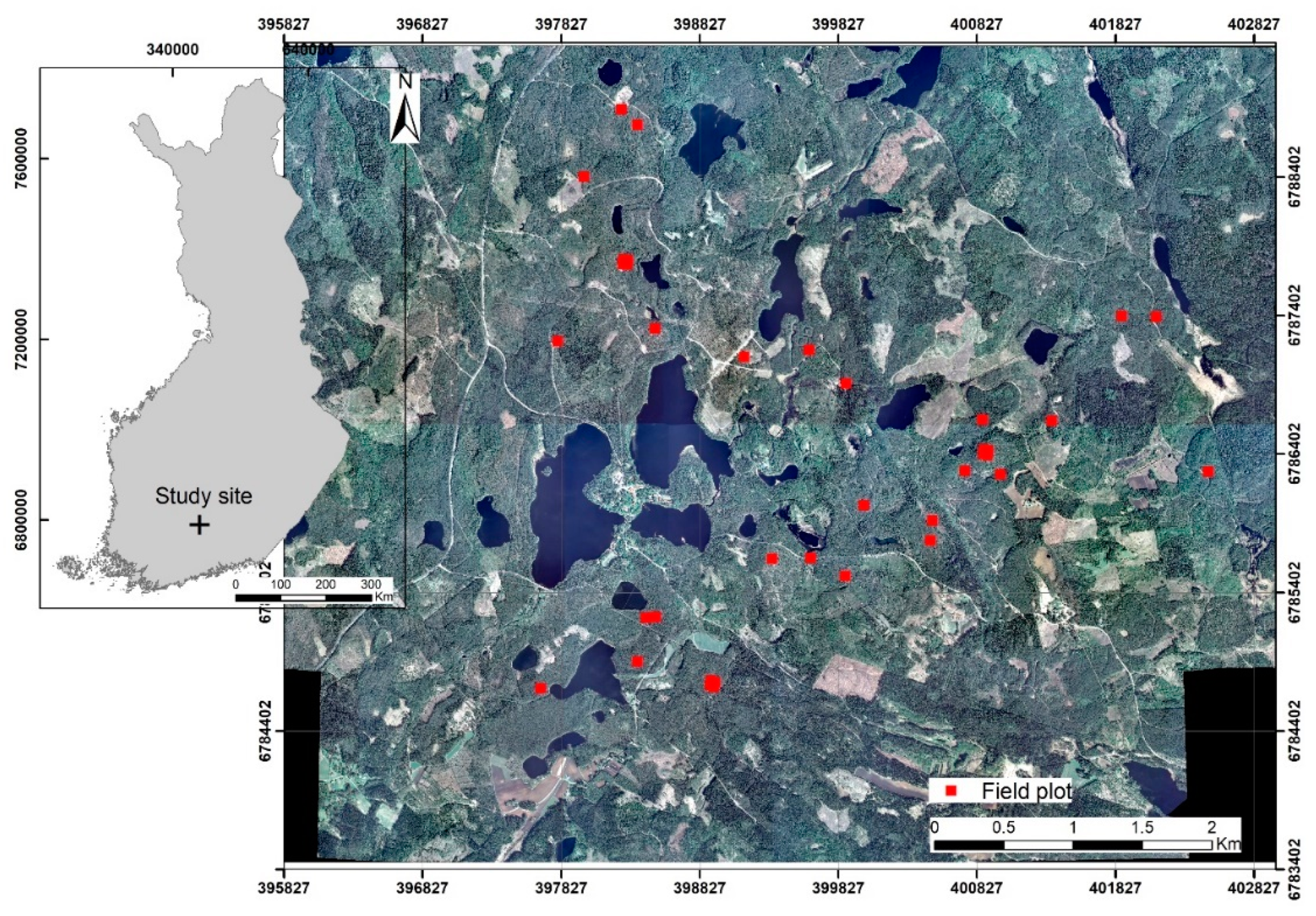
The study area of approximately 2000 ha is located in southern Finland (61.19° N, 25.11° E) and includes both managed and natural southern boreal forests where the main tree species are Scots pine (Pinus Sylvestris L.), Norway spruce (Picea abies (L.) Karst) and silver and downy birches (Betula pendula and pubescens L.). There is no substantial variation in elevation, as it ranges between 125 m and 185 m above sea level.

In 2014, 91 square sample plots with a size of 1024 m² were established in the study area (Figure 1). Locations of the field sample plots were selected based on canopy density and height information derived from airborne laser scanning data in order to cover the variation in these attributes within the study area. All trees with DBH ≥5 cm within the plots were measured using traditional field measurement practices [25] and a total of 2351 Scots pines were identified from 37 of these sample plots that were dominated by Scots pine. The basal-area weighted mean diameter varied between 14.8 and 32.0 cm in these 37 sample plots, development class from young-managed to regeneration-ready stands, and site type from mesic heath to xeric heath forest. In addition, TLS data were acquired in these plots using a Leica HDS6100 (Leica Geosystems AG, Heerbrugg, Switzerland) in the summer of 2014. The plots were scanned as they are (i.e., no removal of lower tree branches or undergrowth vegetation carried out). Point clouds were obtained from five locations (i.e., plot center and four quadrant directions) (Figure 2) with “High-density” mode providing the angle increment of 0.036° in both horizontal and vertical directions and point spacing of 15.7 mm at 25 m from the scan location. Artificial reference targets (i.e., white spheres with a radius of 198 mm) were used to co-register and combine separate point clouds into one, plot-specific point cloud with an average registration accuracy of 2.1 mm.

The global coordinates (i.e., ETRS89-TM35FIN) of reference targets were recorded using two reference points in open areas near the plots (e.g., road, lakeshore, clearing) using a Trimble R8 Global Navigation Satellite System (GNSS) receiver with real-time kinematic signal correction. A Trible 5602 DR200+ total station was used to establish a survey point inside each plot by measuring the distances and angles to the reference points and then measured the locations of the reference targets from the survey point using the total station. This enabled transforming the TLS point clouds into global coordinate system.

2.2. Taper Curve Measurements from TLS Data

To identify Scots pines from TLS point clouds, we applied an approach that has been used in detecting individual trees from point clouds originating from airborne laser scanning [42,43]. First, an iterative triangulation algorithm [44] was applied to a plot-specific point cloud in classifying ground points to generate a digital terrain model (DTM) with 50 × 50 cm resolution. A digital surface model (DSM) with similar resolution was generated using highest points within each raster cell. The normalized canopy height model (CHM) was obtained by subtracting the DTM from the DSM. 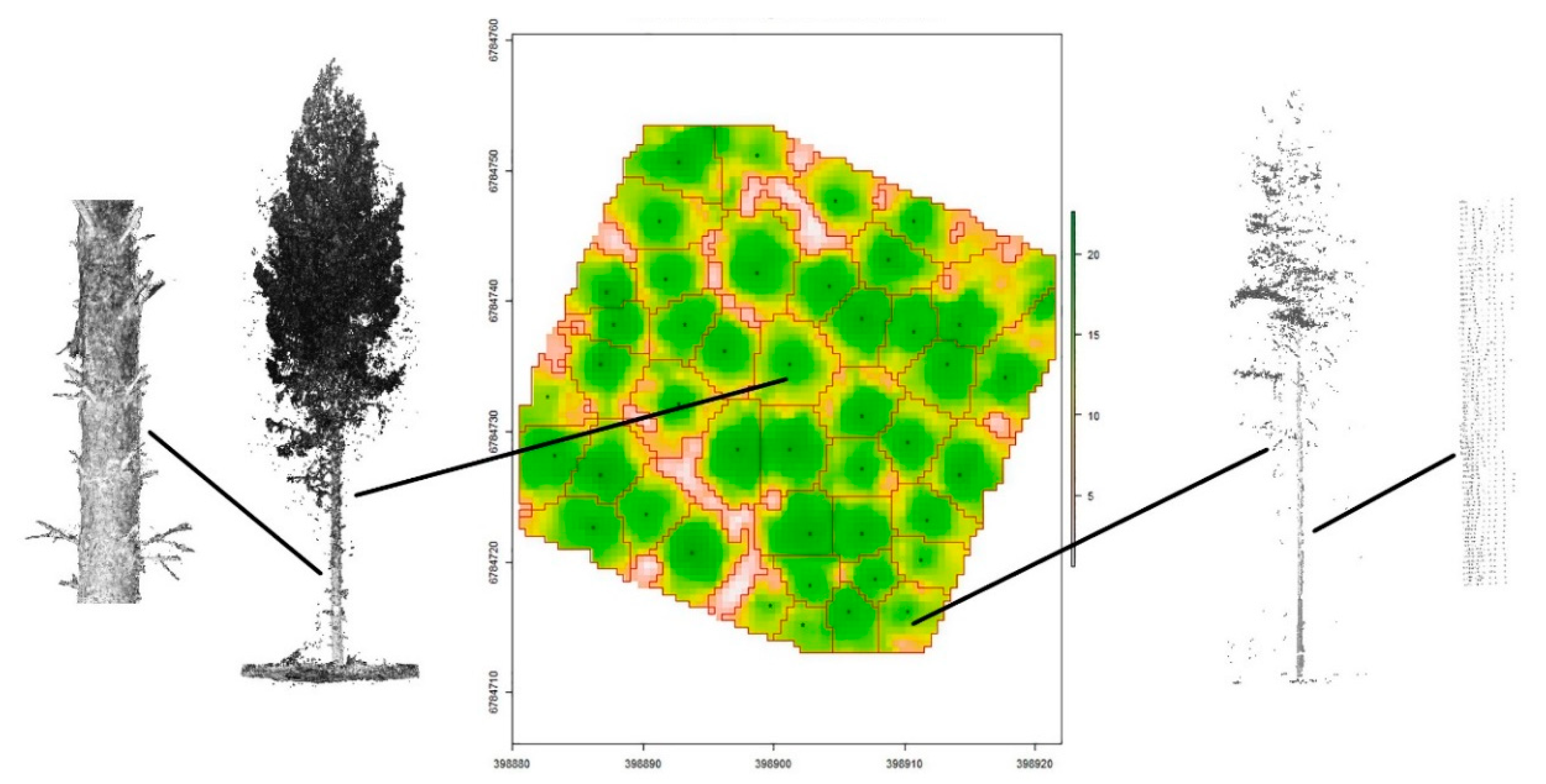The CHM was then segmented to identify individual trees by applying a watershed segmentation algorithm in ArcMap 10.5 where a flow direction of each cell is calculated after the CHM has been negated (see more about the method in [45,46]). Scots pines were visually identified from the segmented point clouds based on the visibility and comprehensiveness of the point cloud. In other words, a visual inspection was undertaken to ensure the quality of point clouds characterizing individual trees and stem as comprehensively as possible to ensure as reliable automatic taper curve measurements as possible. It was observed that point clouds of individual trees were more exhaustive around plot center as it was covered from several scan locations and enabled improved characterization of individual trees (Figure 3). In [16] it was concluded that average point spacing of 6.2 mm on stem surface was sufficient for reliable volume estimates.

Point clouds of the identified Scots pines (i.e., modelling pines) were used to derive a taper curve. Points originating from a stem were automatically classified and separated from points originating from branches following the approach described in [47]. Diameter measurements from the stem points were then automatically derived by fitting circles every 10 cm along a stem. To remove clear outliers from other diameter observations of a taper curve, each automatically derived diameter was compared to the mean of the previous (or following if at the stem base) diameters. If the diameter in question differed more than 4 or 2 cm below or above the breast height, respectively, of the mean of previous (or following) observations it was defined as an outlier. The final TLS-based diameters (i.e., TLS-based taper curves) were used in modelling (Section 2.3).

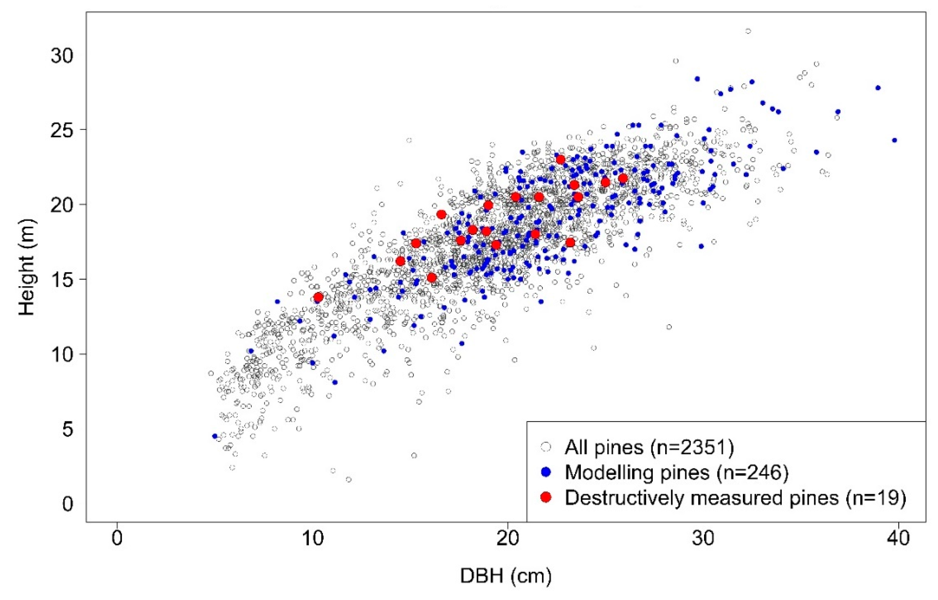
Scots pines with automatic taper curve measurements were matched with the field measurements undertaken in 2014 based on their x and y coordinates. The tree locations were based on TLS data, in other words, stems were manually identified from the TLS point clouds to produce initial stem maps that were finalized (i.e., removing commission errors and adding omission errors) during the field measurements. This enabled us to utilize the field measured tree height in the modelling as TLS-based height can be expected to be underestimated even when acquisition is planned to cover trees in question as comprehensively as possible [16]. Finally, 246 Scots pines were included in the modelling data set, their descriptive statistics are presented in

Table 1. Descriptive statistics of diameter-at-breast height (DBH) and height for all Scots pines within the 37 sample plots (n = 2351), the modelling (n = 246), and destructively (n = 19) pines. Min = minimum, 1Q = 25% percentile, 3Q = 75% percentile, max = maximum.

	Attribute	Min	1Q	Median	Mean	3Q	Max	Standard Deviation
All Scots pines	DBH (cm)	4.8	15.7	19.9	19.4	23.5	39.8	6.2
	Height (m)	1.6	15.0	17.9	17.5	20.8	31.6	4.4
Modelling pines	DBH (cm)	5.0	18.9	22.0	22.3	25.8	39.8	5.6
	Height (m)	4.5	16.5	19.3	19.2	22.0	28.4	3.8
Destructively measured pines	DBH (cm)	10.3	17.1	19.4	19.6	23.0	25.9	4.0
	Height (m)	13.8	17.4	18.3	18.8	20.5	23.0	2.4

and their distribution in relationship to all Scots pines within the 37 sample plots (n = 2351) is depicted in Figure 4.

2.3. Validation Data

An independent data set was used for validating the prediction accuracy of the parametrized taper curve equation. The validation data included 19 Scots pines that were measured in the summer of 2010. These Scots pines were randomly selected from previously (in 2007 and 2009) established sample plots to cover a range of DBH classes of 10–26 cm in the plots in question. More detailed description about sample plots from which these Scots pines were selected can be found in [48]. DBH was defined as a mean of two diameters measured with steel calipers from perpendicular directions at 1.3 m above ground. A Vertex clinometer was used for determining tree height. Variability of validation pines is presented in Table 1.

The trees were cut down as close to the root collar as possible and pruned. For these Scots pines, the diameters were measured at the stump height, height between the stump and 1 m, at 1.3 m, 2 m, and then every meter from perpendicular directions and the mean of each diameter pair was used as the final diameter for each height. A smoothing cubic spline function [49] was fitted to the measured diameters to level unevenness in the diameter measurements caused by, for example, branch knots and bark roughness. For the value of a smoothing parameter, defining the flattening of the cubic spline, 0.4 was selected as it has been proven to be suitable for trees in that region [16]. The smoothing cubic spline function was used for destructively measured Scots pines to derive diameters at various heights using an interval of 0.625% of a tree height. In other words, the diameter in every stem section of 0.625% of a tree height along the stem was obtained, starting from the relative height of 0.625% of a tree height. This interval was selected as it corresponded approximately to the 10 cm measurement interval used for the TLS-derived diameter data for the destructively measured trees. These diameters were then used to calculate the stem volume in stem sections with Huber’s formula [50], and the total stem volume was the sum of these volumes. The length of a stem section was defined based on tree height and the interval of diameters (i.e., 0.625%).

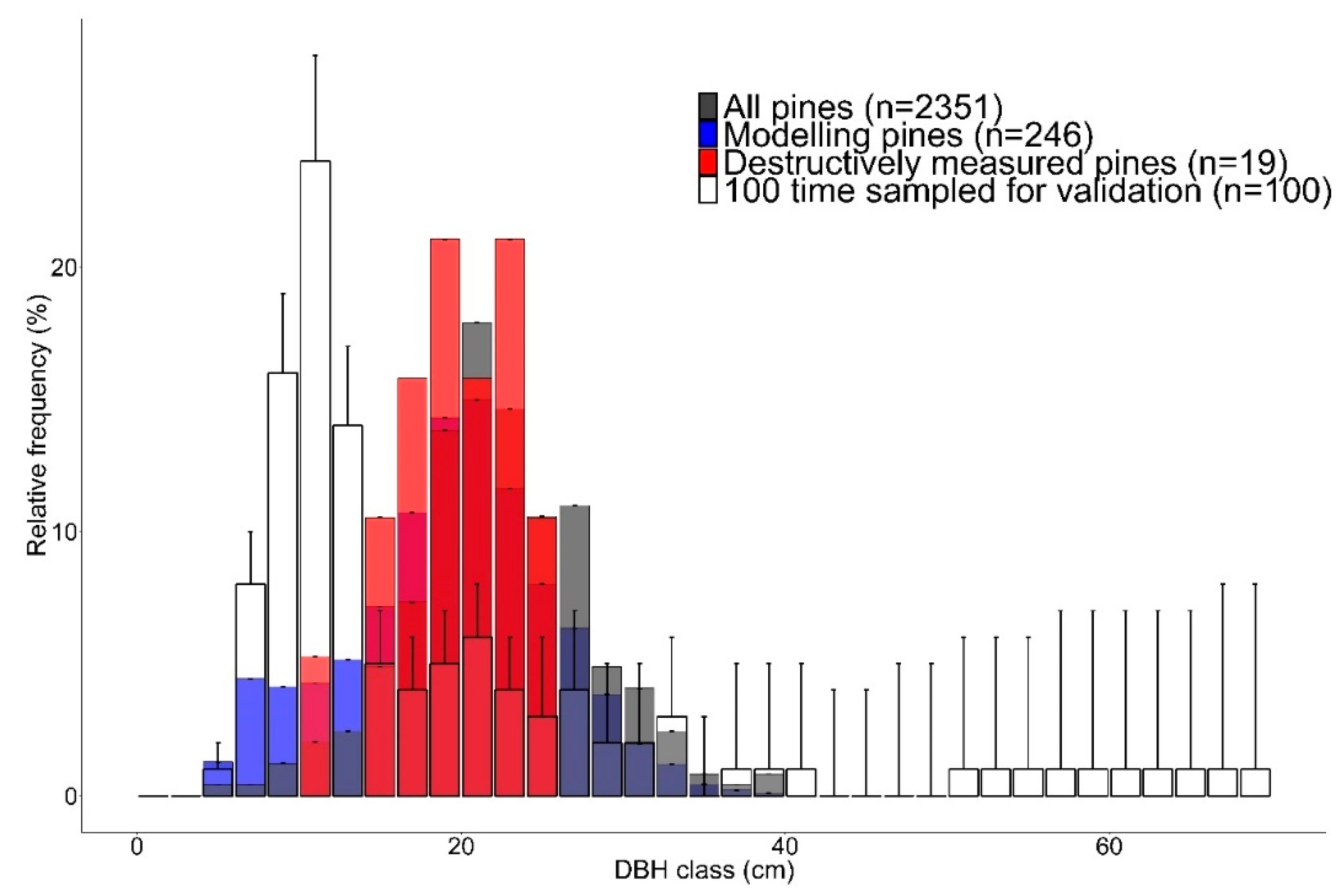
The range in DBH was larger for modelling pines than for validation pines and the DBH classes larger than 25 cm were missing in the validation data set whereas 24% of the modelling pines had a DBH larger than 25 cm (Figure 5). Based on the Shapiro–Wilk test, distributions of DBH classes were not normally distributed for destructively measured, modelling, or all Scots pines (p value < 0.01) and the skewness values for the distributions were 1.90, 1.72, and 1.45, respectively.

In addition to the destructively measured pines, 100 Scots pines with taper curves based on TLS were randomly sampled without replacement 100 times to follow the idea by [51] and increase the reliability of the validation data set. Figure 5 represents the mean DBH distribution of the 100 repeated sampling of TLS-based validation pines as well as the standard deviation of the distribution. The Shapiro–Wilk test revealed that the mean distribution did not follow normal distribution (p value <0.01) and the skewness for the distribution was 2.53. The reference stem volumes of these Scots pines were obtained by fitting a smoothing cubic spline function [49] to the TLS-based taper curve measurement and utilizing Huber’s formula [50], similarly to the destructively measured trees, for stem sections with a length of 10 cm.

2.4. Modelling

A smoothing cubic spline function was fitted for every modelling pine included in the sample by utilizing TLS-based taper curves with the same smoothing parameter (i.e., 0.4) as for the validation pines. To obtain also diameters in a crown where occlusion is hindering automatic diameter derivation, the field-measured height was used to ensure the cubic spline would produce 0 cm at tree height. The created spline functions were applied in deriving diameters for relative heights of 0%, 1%, 2.5%, 5%, 7.5%, 10%, 15%, 20%, 25%, 30%, …, 95%, and 100% for each Scots pine separately following the approach in [29].

In many of the taper curve modelling studies, ratio between a diameter at certain height and other diameters have been used as the response variable, and this approach was also applied in this study. The ratios between the diameter at 20% relative height and all other diameters at each relative height are the response variable of the taper curve equation. Following the equation form in [29] we used a polynomial equation with powers following the Fibonacci series (Equation (1)):

$$\frac{d_l}{d_{2h}}=b_{1}x+b_2{x}^2+b_3{x}^3+b_4{x}^5+b_5{x}^8+b_6{x}^{13}+b_7{x}^{21}+b_8{x}^{34}$$

(1)

where d_l is the diameter at a relative height of l from the ground, d_.2h is the diameter at 20% relative height, and x is the relative distance from the tip of a tree.

In addition, the predictor variable (i.e., the relative height from the top) was calculated for each relative height and every sample tree, separately. The taper curve equation by [29] was developed based on the mean ratios between the diameter at the 20% relative height and diameters from other relative heights and this approach was also adopted in this study. Linear regression analysis was used for these mean ratios for estimating coefficients for the predictor variable for Scots pine with the various sample size.

To test the effect of the sample size on the volume estimates, in addition to including all 246 modelling pines, we decreased the sample size by randomly selecting (without replacement) 221, 196, 171, 146, 121, 96, 71, 46, 21, 15, 10, 5, and 1 Scots pines from the modelling data at a time. We then estimated the coefficients for the taper curve equation presented in Equation (1) for each sample size. Randomized sampling without replacement was performed 100 times for each sample size to investigate the effect of sampling error on the modelling.

2.5. Evaluation of Results

Stem volume was estimated for the validation Scots pines (both 19 field-measured and 100 times 100 randomly sampled TLS-measured) using the parametrized taper curve equation based on all modelling pines as well as the different number of randomly sampled modelling pines mentioned above. The stem volume was obtained similarly to the validation data, in other words Huber’s formula was applied for 10 cm stem sections using diameters obtained from the parametrized taper curve equation. Student’s t-test was used for assessing the difference between stem-volume estimates for validation pines based on taper curve equation parametrized with various sample sizes. The RMSE and mean difference between the reference stem volume of the validation pines and the stem-volume estimates based on parametrized taper curve equation were calculated (Equations (2) and (3)):

$$RMSE \left({\mathrm{dm}}^3\right)=\sqrt{\frac{\sum {\left(v_{ref}-v_{pred}\right)}^2}{n}}$$

(2)

$$\mathrm{Mean}\mathrm{difference}\left({\mathrm{dm}}^3\right)=\frac{\sum v_{ref}-v_{pred}}{n}$$

(3)

where n is the sample size, V_ref is the stem volume calculated based on the taper curves measured with the validation pines (i.e., destructive measurements) and V_pred is the stem volume estimated with taper curve equation parametrized based on taper curves measured automatically from the TLS point clouds. The RMSE and mean difference were divided by the mean volume based on taper curves measured from validation pines and multiplied by 100 to obtain the relative RMSE and mean difference.

To assess the effect of the random sampling between sample sizes, we calculated minimum, maximum, mean and standard deviation of absolute and relative RMSE and mean difference of each sample size that were randomly selected 100 times. Additionally, difference between the mean taper curve of validation pines and taper curves based on the parametrized equation predicted with (i) all Scots pines, (ii) 96 Scots pines, and (iii) only one Scots pine was assessed. The taper curves were calculated as a mean of the taper curve estimates based on the random sampling of modelling pines that was repeated 100 times for (i) and (ii). The difference (i.e., error) between the estimated and the reference taper curve was obtained by subtracting the reference taper curve from the estimates. Furthermore, the relationship between reference and estimated stem volume based on the taper curve equation that was parametrized with (i) all (n = 246), (ii) 96, and (iii) one Scots pine was assessed including the variation affected by due to the sampling of reference Scots pines, with reference volume obtained based on the TLS-based taper curves, 100 times.

To assess the reliability of the stem-volume estimates obtained with the parametrized taper curve equation, we also calculated both absolute and relative RMSE and mean difference of stem-volume estimates of validation pines using the existing taper curve equation for Scots pine by [29].

3. Results

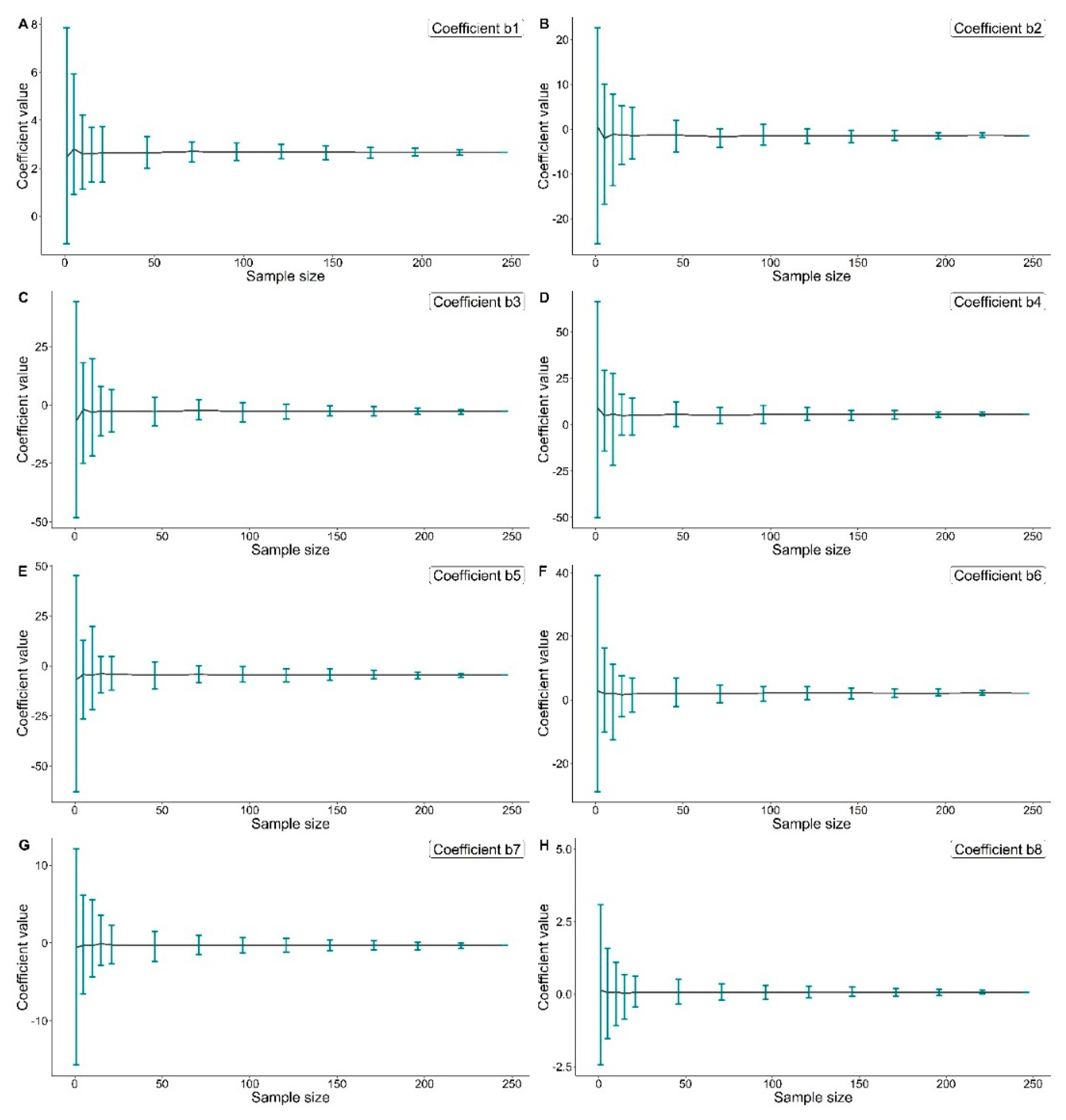
The mean values for coefficients of the taper curve equation were rather similar when the sample size was at least 96 Scots pines (Figure 6). However, there was evident variation in the range of coefficients, especially when the sample size was <46 Scots pines. Despite this variation, Student’s t-test revealed statistically significant difference (p-value ≤ 0.05) between volume estimates based on the parametrized taper curve equation using sample sizes at least 10 Scot pines. The stem-volume estimates between the parametrized model using 5 or 1 Scots pine were not significantly different (p-value > 0.05).

The effect of random sampling, which was performed 100 times, was assessed by calculating absolute and relative RMSE as well as mean difference of stem-volume estimates that were based on the re-parametrized taper curve equation using varying sample size. The mean RMSE was ≤52 dm³ when the sample size included at least 10 Scots pines corresponding to the relative mean RMSE of ~21% (

Table 2. Absolute and relative root mean square error (RMSE) and mean difference of volume estimates based on parametrized taper curves obtained with samples of varying sizes that were randomly selected 100 times. Min = minimum, Max = maximum, Mean = average, Std = standard deviation.

		RMSE								Mean Difference
		dm3				%				dm3				%
		min	max	mean	std	min	max	mean	std	min	max	mean	std	min	max	mean	std
Sample Size	1	29.2	156.3	71.6	30.0	12.0	62.5	29.6	12.3	−126.3	70.5	−31.6	39.3	−49.3	28.6	−13.1	16.3
	5	27.0	109.7	57.4	18.7	11.8	46.7	23.6	7.2	−76.7	21.3	−26.0	20.2	−31.0	9.7	−10.7	8.2
	10	28.8	130.7	51.8	14.8	12.6	49.5	21.3	5.6	−56.8	15.4	−21.1	14.3	−23.1	5.9	−8.7	5.8
	15	28.4	119.3	51.4	14.4	12.3	45.2	21.2	5.5	−48.7	3.0	−21.9	10.9	−19.4	1.2	−9.0	4.4
	21	28.4	119.1	51.2	14.1	11.8	45.1	21.1	5.4	−48.4	4.5	−21.9	10.3	−20.6	1.8	−9.1	4.2
	46	29.3	117.8	50.5	13.5	12.1	44.6	20.8	5.0	−45.6	0.7	−21.6	8.4	−17.8	0.3	−8.9	3.2
	71	28.9	116.0	50.7	13.3	12.6	43.9	20.8	4.9	−44.2	−5.8	−21.8	7.8	−17.8	−2.5	−8.9	3.0
	96	32.6	117.2	50.8	13.1	13.5	44.4	20.9	4.8	−45.6	−9.2	−22.2	7.1	−17.3	−4.0	−9.1	2.7
	121	31.1	116.2	50.6	13.2	12.9	44.0	20.8	4.8	−43.2	−8.2	−22.1	6.8	−18.4	−3.4	−9.1	2.6
	146	30.7	115.3	50.6	13.4	12.7	43.7	20.8	4.9	−46.4	−7.7	−22.0	7.3	−19.1	−3.2	−9.1	2.8
	171	29.8	117.9	50.4	13.4	12.4	44.6	20.7	4.9	−46.1	−5.0	−21.7	6.9	−17.3	−2.1	−8.9	2.6
	196	30.9	121.0	50.4	13.4	12.8	45.8	20.7	4.9	−48.9	−8.3	−21.8	6.8	−18.5	−3.4	−8.9	2.6
	221	31.7	119.5	50.4	13.3	13.1	45.3	20.7	4.9	−46.8	−9.5	−21.8	6.5	−17.7	−3.9	−9.0	2.4
	246	30.6	122.3	50.5	13.2	12.7	46.3	20.8	4.8	−50.9	−7.2	−21.8	6.4	−19.3	−3.0	−9.0	2.4

). The standard deviation of absolute and relative RMSE followed a similar pattern and were ≤15.8 dm³ and 5.6%, respectively, when sample size was ≥10 Scots pines. Also, the mean absolute and relative mean difference were −22 dm³ and 9%, respectively, when the sample size was ≥10 Scots pines. However, the standard deviation of mean difference increased from 10.9 dm³ to 14.3 dm³ (from 4.4% to 5.8%) when the sample size decreased from 15 to 10 Scots pines.

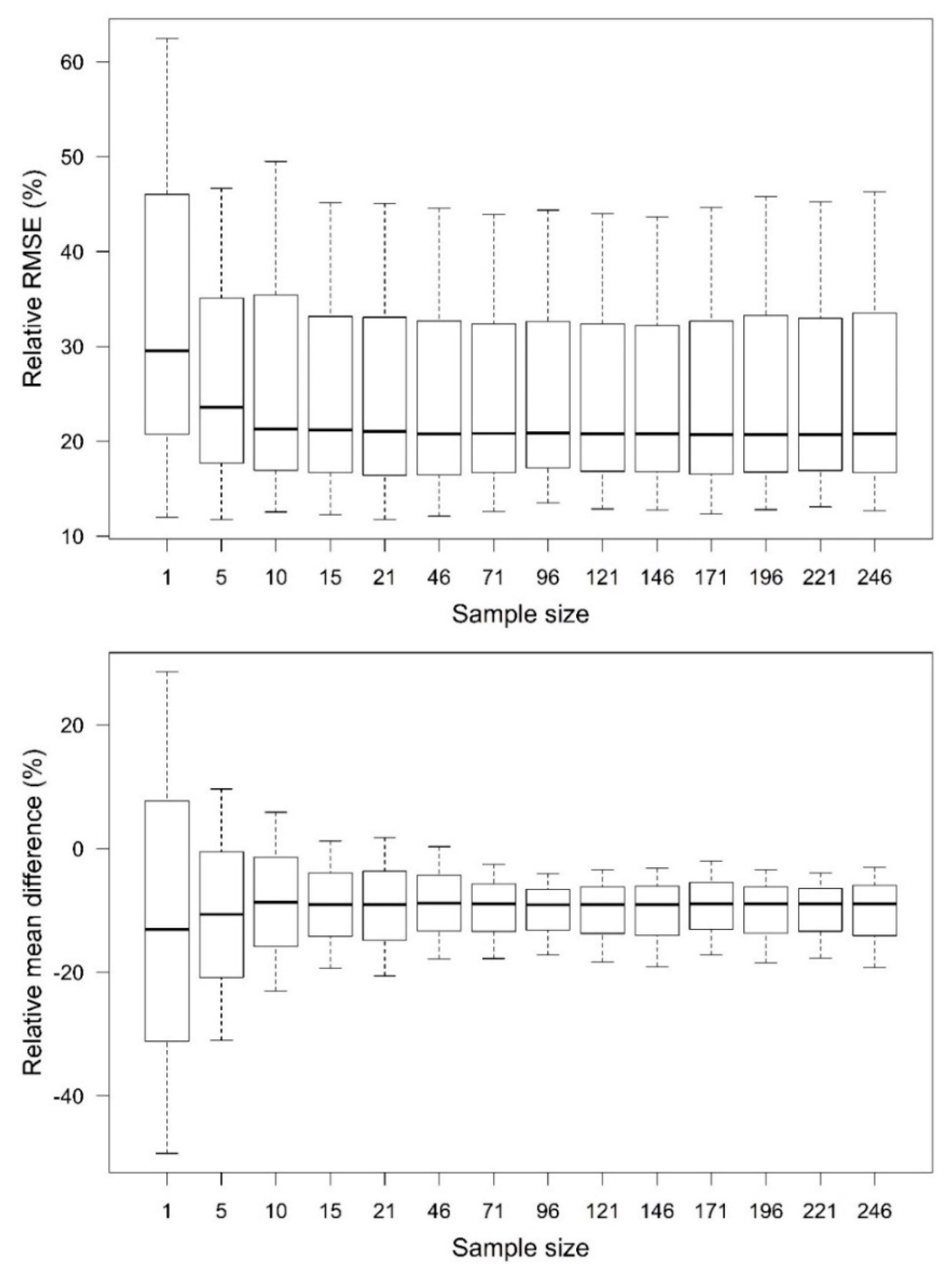
The variation in relative RMSE of stem-volume estimates was rather similar when at least 15 Scots pines were included in parametrizing the taper curve equation and sample size of 96 Scots pines produced smallest range in relative RMSE (Figure 7). The variation in relative mean difference, on the other hand, fluctuated more between sample sizes, but smallest visible variation was obtained with the sample sizes of 96 and 221 Scots pines (Figure 7). It should be noted, however, that standard deviation of relative mean difference was ≤3.2% for sample sizes of 46 modelling pines or less whereas it remained ≥4.2% for larger sample sizes (Table 2). The standard deviation of mean relative RMSE, on the other hand, was relatively stable at approximately 5.0% when at least 46 Scots pines were included in the parametrization but increased especially when the sample included less than 21 Scots pines (Figure 7, Table 2).

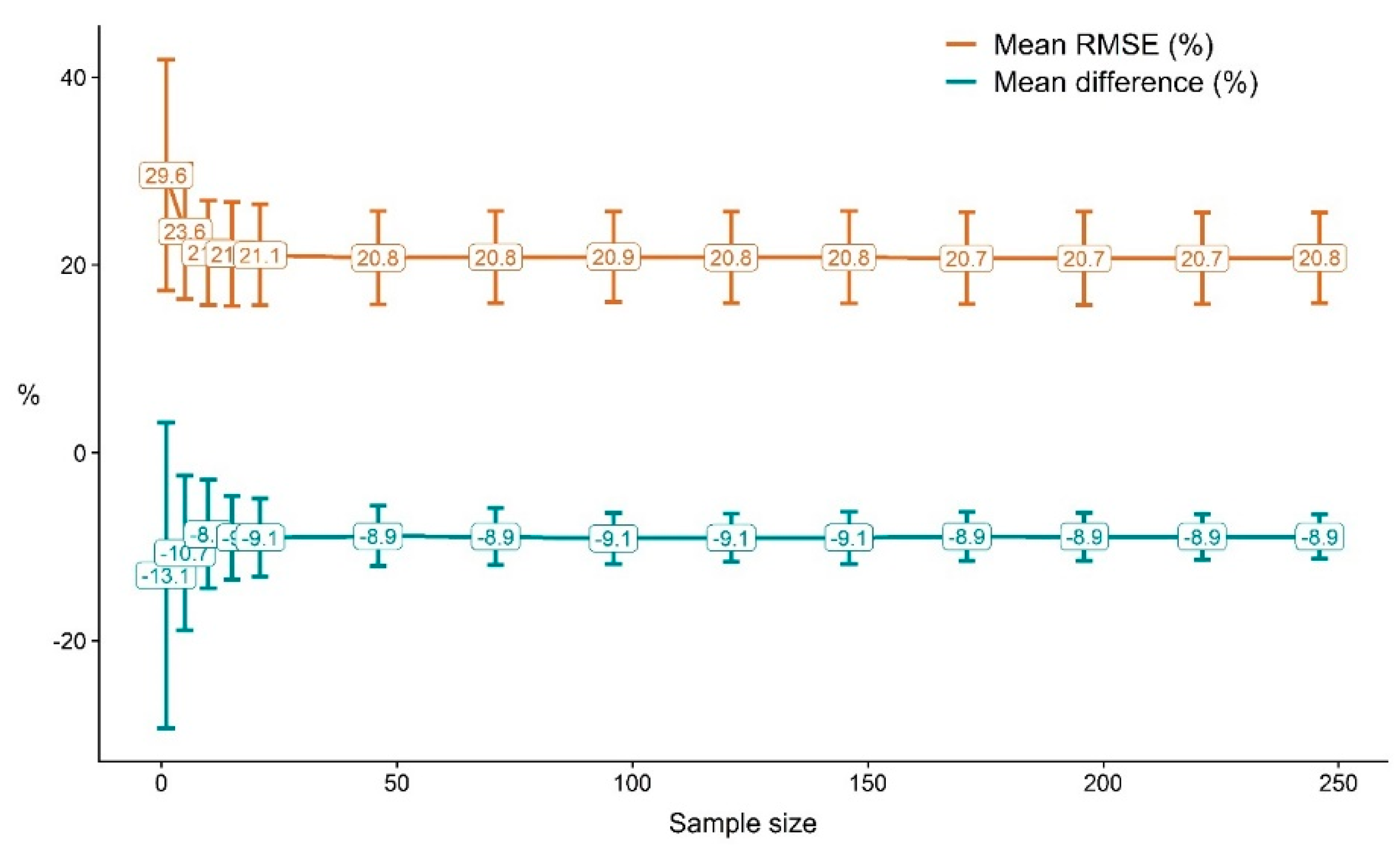
The mean relative RMSE was approximately 21% with all other sample sizes except the smallest ones (i.e., 5 and 1 Scots pines) similarly to the mean relative mean difference of ~9% throughout the sample sizes (Figure 8). Similarly, the standard deviation of the relative RMSE was visibly different for the smallest sample sizes whereas the standard deviation of the relative mean difference increased visibly when the sample size decreased from 46 to 21 Scots pines.

The variation in relative RMSE and mean difference with also large sample sizes (Figure 7; Figure 8, Table 2) was due to the sampling also of reference data from the Scots pines measured from TLS data. In other words, even though all 246 Scots pines were included in the parametrizing the taper curve equation, in addition to the 19 destructively measured Scots pines, 100 randomly sampled Scots pines (repeated 100 times) were included in the validation data sets, causing the variation in the accuracy assessment. As the total area of the 37 sample plots correspond to ~0.2% of the entire 2000 ha study area, it can be approximated that 46 modelling pines coincide ~0.003% of the Scots pine population within the study area.

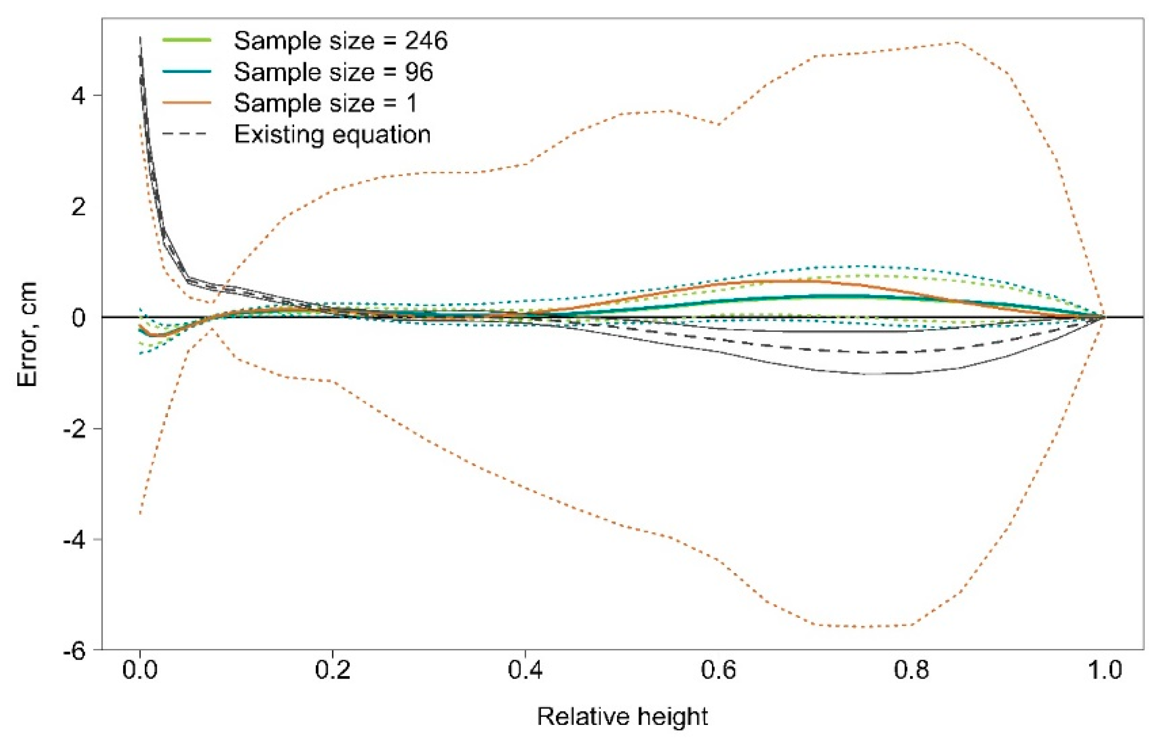
There was no visible difference between the taper curve estimate based on the parametrized taper curve equation when all 246 or 96 or even 1 modelling pines that were randomly selected 100 times were included in the parametrization (Figure 9). However, minimum and maximum errors of estimated taper curves varied notably if only 1 Scots pine was used for parametrization whereas the errors were not as visible when taper curves based on 96 and 246 Scots pines are examined. The parametrized taper curves mainly produced larger diameters when compared to the reference taper curve, only at the lowest relative heights the estimated diameters based on the parametrized taper curves were smaller than the reference taper curve. These differences in the taper curves help explain the overestimates in the stem volumes based on the parametrized taper curve equation.

To examine the overestimation in more detail, Figure 10 shows the relationship between the reference volume and predicted stem-volume estimates when all (n = 246), 96, or 1 Scots pine were included in the parametrizing the taper curve equation. Volume was mainly overestimated throughout the volume range, but it is especially visible for small trees as they were more present in the sampled reference Scots pines (Figure 5). Also, as the sampling of the 100 randomly selected reference Scots pines was repeated 100 times and increment of variation in the volume estimates is visible in Figure 10b,c showing a similar trend to the results presented above.

The RMSE of stem-volume estimates based on the taper curve equation by [29] was 31.46 dm³ (18.95%), which is in same magnitude than the RMSEs obtained from the parametrized taper curve equation based on the TLS data. The mean difference of 3.69 dm³ (1.52%), however, was notably different when compared to the mean difference of stem-volume estimates obtained by parametrizing the taper curve equation with our TLS data. Taper curve based on the existing equation (i.e., coefficients estimated in [29]) produced smaller diameters throughout the relative heights, except for the lowest relative heights (Figure 9).

4. Discussion

Although the mean difference of the stem-volume estimates was somewhat similar between estimates from taper curve equation parametrized using different sample sizes, there was an increase in its standard deviation when sample size was less than 46 Scots pines. Similarly, the relative RMSE of stem-volume estimates increased when the sample size was less than 46 Scots pines. These results suggest that a minimum of 46 Scots pines are required to parametrize an existing Scots pine taper curve equation for our study area. This can be relevant when sampling for generating volume equations is planned, as the number of Scots pines included in modelling data could be decreased.

The relatively constant overestimate of 9.0% can be at least partly explained by the discrepancy between modelling and validation data sets. The destructively measured data set lacked large DBH classes whereas 24% of the modelling pines were larger than 25 cm in DBH. In addition, random sampling of reference Scots pines from the modelling data resulted in data sets that mainly included Scots pines with DBH < 15 cm (Figure 5). This is also supported by the findings of [52] where samples that did not adequately represent the population resulted in unreliable stem-volume estimates. A priori knowledge based on airborne laser scanning, for example, could have been used in characterizing height variation within the population and optimizing the selection of sample trees to better include the variation of the entire Scots pine population within the study area. That way, TLS data acquisition could have been planned according to an optimal scan distance of a maximum of 50% of the tree height as proposed by [16], to obtain as comprehensive point cloud as possible to ensure accurate taper curve measurements. This kind of setup for TLS data acquisition decreased the relative mean difference of stem-volume estimates to even as low as 0.9% in our previous study [16] in the same study area when using the same terrestrial laser scanner.

The Scots pines used for modelling were visually identified from the TLS point clouds to ensure the quality of the point clouds in covering the trees as comprehensively as possible. As the accuracy of diameter measurements at various heights from TLS point clouds has been demonstrated in previous research in the same study area [16,18,22,28], it was not investigated in this study. However, we do acknowledge that reliability of diameters from different heights varies when producing taper curves [16], especially when occlusion hinders the laser beam to hit a stem within a crown and this was also demonstrated in Figure 9. Additionally, the reliability of TLS-based diameters towards the tip of a tree decreases due to the increase of the distance between the scanner and a stem when the laser can hit a branch instead of the stem due to the laser beam divergence [53]. Thus, research on acquiring TLS point clouds from trees identified for modelling specifically would be needed to understand how scanner (phase-shift vs time of flight) affects taper curve measurements. Furthermore, investigating of utilization of more than one cubic spline function in generating final taper curve would be of interest.

Although, the maximum number of modelling pines used in this study was rather modest compared to the data sets included in [29] or reported in [13], our study area only covered approximately 2000 ha and our aim was not to develop a comprehensive, ready-to-apply taper curve equation for the whole Finland, which was the main objective in [29]. Additionally, sample sizes similar to this study have been reported when species-specific national or provincial stem-volume models have been developed [36,54,55]. Furthermore, in [37] it was concluded that the minimum number of sample trees was 15 and 30 for jack pine (Pinus banksiana Lamb.) and black spruce (Picea mariana (Mill.) B.S.P), respectively across the boreal forest of Northern Ontario when estimating coefficients for an existing stem taper model, whereas in [38] reliable stem-volume estimates were obtained with 36 eucalyptus trees from ~559 ha. Our results are thus in line with these as we obtained relatively stable RMSE of stem-volume estimates with a sample size of ≥46 trees, which corresponds approximately 0.003% of the Scots pine population within our 2000 ha study area. In [51], TLS was used to provide DBH and tree height for estimating coefficient of biomass equation and they reported that more than 100 trees for a study area of ~26 ha were required for stable estimates of coefficients. Nevertheless, one of the limitations of our study is that the data were acquired from rather small area and more investigations are needed to understand whether these findings are true also for other tree species, larger scale (e.g., nationally), and/or more diverse areas. Traditional stem analysis from destructively sampled trees is time consuming and impractical in many places (e.g., urban and conservation areas) whereas TLS provides similar information without the need for destructive measurements. Comparable results of ours and the above-mentioned studies indicate the suitability of TLS data for parametrizing an existing taper curve model compared to traditional means.

Our hypothesis about decreasing the number of modelling trees from hundreds to tens, while still maintaining the same level of reliability, was supported as 46 Scots pines resulted in similar relative RMSE and mean difference compared to when all 246 Scots pines were included in the parametrizing. The number of Scots pines used for parametrizing the existing taper curve equation seems to have little effect on stem-volume estimates as the standard deviation of mean difference was ≤3.2% regardless of the sample size when at least 46 Scots pine were included. As resources for acquiring adequate data sets for modelling stem volume and biomass can be limited, the results of this study indicate that sample size may not be as important as has been suggested for obtaining stem-volume estimates based on a taper curve equation with small variation. Additionally, TLS-based point clouds offer a feasible means for data acquisition for detailed taper curve measurements to overcome limitations associated with destructive sampling. TLS reduces field work as data from same sample size can be obtained more efficiently [16]. Furthermore, data acquisition from conservation areas, for example, is only possible when destructive measurements are not required. Finally, multi-temporal TLS measurements enable monitoring of stem taper over time [56].

5. Conclusions

In this research, we assessed how TLS-based point clouds offered detailed taper curve measurements for investigating the effect of the number of sample trees on the parametrization of an existing taper curve equation as well as on stem-volume estimates obtained with the equation. We observed that there was consistency in the RMSE of stem-volume estimates as it remained ≤20.9% when at least 46 Scots pines were used for parametrizing the existing taper curve equation. Furthermore, the mean difference in stem volume was not affected by the sample size and its standard deviation remained ≤3.2% when the sample included at least 46 Scots pines. These results support our hypothesis that the required sample size for parametrizing an existing taper curve equation for obtaining consistent volume estimates is only tens of samples instead of hundreds, which has been commonly suggested. In addition to traditionally used DBH and tree height, TLS provides a feasible means of acquiring information about stem tapering without destructive measurement. Thus, it can be concluded that the sample size can be decreased from hundreds to below 50 trees but still obtain consistent stem-volume estimates for our study area when TLS-derived taper curves were used.