1. Introduction
Forest canopy structure can be defined as “the organisation in space and time – including the position, extent, quantity, type and connectivity – of the aboveground components of vegetation” [
1]. While the essential function of the forest canopy is to allow plants to capture energy for photosynthesis, and to facilitate the production of reproductive organs such as flowers, fruits and seeds [
2,
3], the biophysical structure of the canopy also constitutes a complex, dynamic habitat for a myriad of other organisms [
4,
5]. The positive correlation between the heterogeneity of this habitat and biological diversity is supported by a wide range of studies; for a review see Tews
et al. [
6]. Canopy structure is also intimately related to important functional characteristics and processes of forests [
7,
8].
Given the ecological importance of the forest canopy, forest managers and researchers require a reliable and cost effective method for detecting and monitoring temporal and spatial changes in this structure. Unfortunately, the measurement of many components of canopy structure can be acutely limited by their inaccessibility, and as a result, most descriptions of structure are by necessity simplifications [
1]. Specialised equipment and techniques for measuring aspects of canopy structure have been used in a number of studies – see for example MacArthur and MacArthur [
9], Horn [
10], Blondel and Cuvillier [
11] – but these methods are often not applicable outside, nor easily repeated within, their respective study areas. As an example, in their review of the literature regarding ‘canopy stratification’, Parker and Brown [
12] found many disparities in the meanings proposed for this term, together with substantial variation in the methods suggested for its measurement. More importantly, the authors were unable to reconcile the results of applying these different methods even within a single, well-studied forest canopy.
By stepping back from the trees in order to better see the forest, many recent advances in quantifying canopy structure have utilised remote sensing technologies. Reviews by Kasischke
et al. [
13]; Treitz and Howarth [
14]; and Lefsky
et al. [
15] provide a useful introduction to these technologies. For example, studies using technologies such as LiDAR (Light Detection and Ranging) to quantify canopy structure have demonstrated strong correlations between remotely-sensed and field-measured data for such attributes as the maximum height of the canopy and canopy volume [
16], as well as individual tree height, stand height and foliage/branch projected cover [
17]. However, the interpretation of remotely-sensed data characterising the
interior of the canopy remains problematic – particularly in taller, ‘closed’ forests – where the density of foliage reduces the penetration of the overstorey canopy by the LiDAR pulses [
18]. The essential problem under such conditions is to determine the appropriate ‘weighting’ of the relatively small number of data points that can be reliably measured at increasing depths beneath the upper surface of the canopy. A number of researchers [
19,
20,
21,
22] have developed ‘canopy height profile’ indices similar to the foliage height diversity index developed by MacArthur and MacArthur [
9]; and subsequent refinements of this technique [
23,
24] to address this problem. Such indices can improve the interpretation of returns from within the canopy since they allow the inference of the presence or absence of vegetation from the smaller number of returns from within this zone, which in turn may reveal the presence of distinct strata. However the selection of these strata should reflect the composition of plants present within the canopy in order to be ‘biologically meaningful’ [
23,
25]. A small number of studies have used remote-sensing technologies (collecting data from single or multiple types of sensor, e.g., LiDAR in combination with multi-spectral imaging) to identify canopy tree species [
26,
27], however the suitability of such methods for delineating meaningful strata within tall, closed canopy, structurally complex forests remains untested.
In this paper we address this knowledge gap and demonstrate a ground-based methodology using inexpensive and easily acquired measurements to quantify and model canopy stratification. The methodology is similar to those developed by other researchers [
28,
29,
30,
31], however there are a number of differences that distinguish our methodology. The development of our methodology was based on the testing and integration of the following steps:
- 1)
The geometry of a free growing tree crown within a forest stand can be predicted on the basis of the diameter at breast height (dbh) of its stem;
- 2)
The effect of competition on free growing crown shape and volume can be modelled using AutoCAD™ software (AutoCAD 2000, Copyright 1982-2000 AutoDesk Inc.) to position and modify neighbouring crowns on the basis of the relative location of their stems;
- 3)
A three dimensional (3D) model of all tree crowns within a forest canopy can be generated using AutoCAD™ and knowledge of the genus, dbh and relative location of each stem;
- 4)
The foliage volumes of tree crowns in the 3D model can be used to identify the presence or absence of different strata within the canopy;
- 5)
The 3D model can be used to identify the plant genera associated with each canopy stratum.
2. Methods
We tested our methodology in the tall (>30 m) wet eucalypt forests of southern Tasmania – structurally complex forests that were likely to be difficult to measure. Tall wet eucalypt forests include tall wet sclerophyll forest and tall mixed forest. The vertical structure of these forests is characterised by distinct strata. The canopies of tall wet sclerophyll forests are dominated by Brown-top Stringybark (
Eucalyptus obliqua [L’Hérit.]) and Swamp Gum (
Eucalyptus regnans [F. Muell.]) over a secondary stratum of trees that typically includes Blackwood (
Acacia melanoxylon [R. Br.]) and Silver Wattle (
Acacia dealbata [Link]). Beneath these strata is an understorey of shrub species, the most widespread of which are Blanket Leaf (
Bedfordia salicina [Labill.]), Musk (
Olearia argophylla [(Labill) Benth.]), Lancewood (
Nematolepis squamea [Labill.] Paul G. Wilson.) and Dogwood (
Pomaderris apetala [Labill.]) [
32]. The stratification within mixed forest stands is similar, but with an understorey of cool temperate rainforest trees including Myrtle Beech (
Nothofagus cunninghamii [Hook.] Oerst.), Southern Sassafras (
Atherosperma moschatum [Labill.]), and Celery-top Pine (
Phyllocladus aspleniifolius [Labill.] Hook. F.) [
33,
34]. At the stand level there can be wide variations in vertical structure. The height attained at maturity varies with altitude, soil fertility and rainfall [
34] and the number of distinct strata and the genera present within each stratum varies with successional stage and/or the number of age classes present. Much of this latter variation reflects differences in the extent and intensity of fires that intermittently occur within wet eucalypt forests [
33,
35,
36].
Four sites were selected from a larger suite of Long Term Ecological Research (LTER) sites established to investigate floristic and structural attributes along a wildfire chronosequence. Further details are available in the establishment report by Turner
et al. [
37]. The four sites have a southerly aspect (
Table 1) and encompass the broad range of age and structural conditions for this forest type. Each site was sampled using a 50 m × 50 m plot which was subdivided into a grid of 10 m × 10 m subplots to facilitate the mapping of individual stems and other structural components.
Table 1.
Environmental parameters of the four study plots.
Table 1.
Environmental parameters of the four study plots.
| | Plota |
| Parameter | 1966S | 1934S | 1898S | OGS |
| Year of regeneration | 1966 | 1934 | 1898b | pre 1895 |
| Aspect | southeast | south | south | south |
| Altitudec | 280 m | 180 m | 160 m | 120 m |
| Topographic position | midslope | midslope | midslope | midslope |
| Site potentiald | 41-55 m | 55-76 m | 55-76 m | 55-76 m |
| Soil parent material | dolerite | dolerite | dolerite | dolerite |
| Dominant tree species | E. obliqua | E. obliqua | E. obliqua | E. obliqua |
Within each 50 m × 50 m plot the following measurements were made: For each woody plant stem >10 cm diameter at breast height (dbh), dbh, species and horizontal coordinates were recorded. For eucalypt stems crown condition (healthy, suppressed or senescent) was also recorded. The height to top of crown and height to base of green crown were measured for a representative sample of free-growing trees from each genus using a hypsometer (Forestor Vertex Hypsometer, Haglöf Sweden). Mean crown width for these trees was estimated using measuring tapes along the widest axis and at 90° to this measurement. Only genera which contributed on average ≥1% of plot basal area were assessed. For each genus a sample of crowns relatively free from the geometric distortions induced by competition and the mortality of individual branches was photographed to aid the selection of a simple geometric figure to describe the crown profile. Field measurements were taken over the period of January through February 2006.
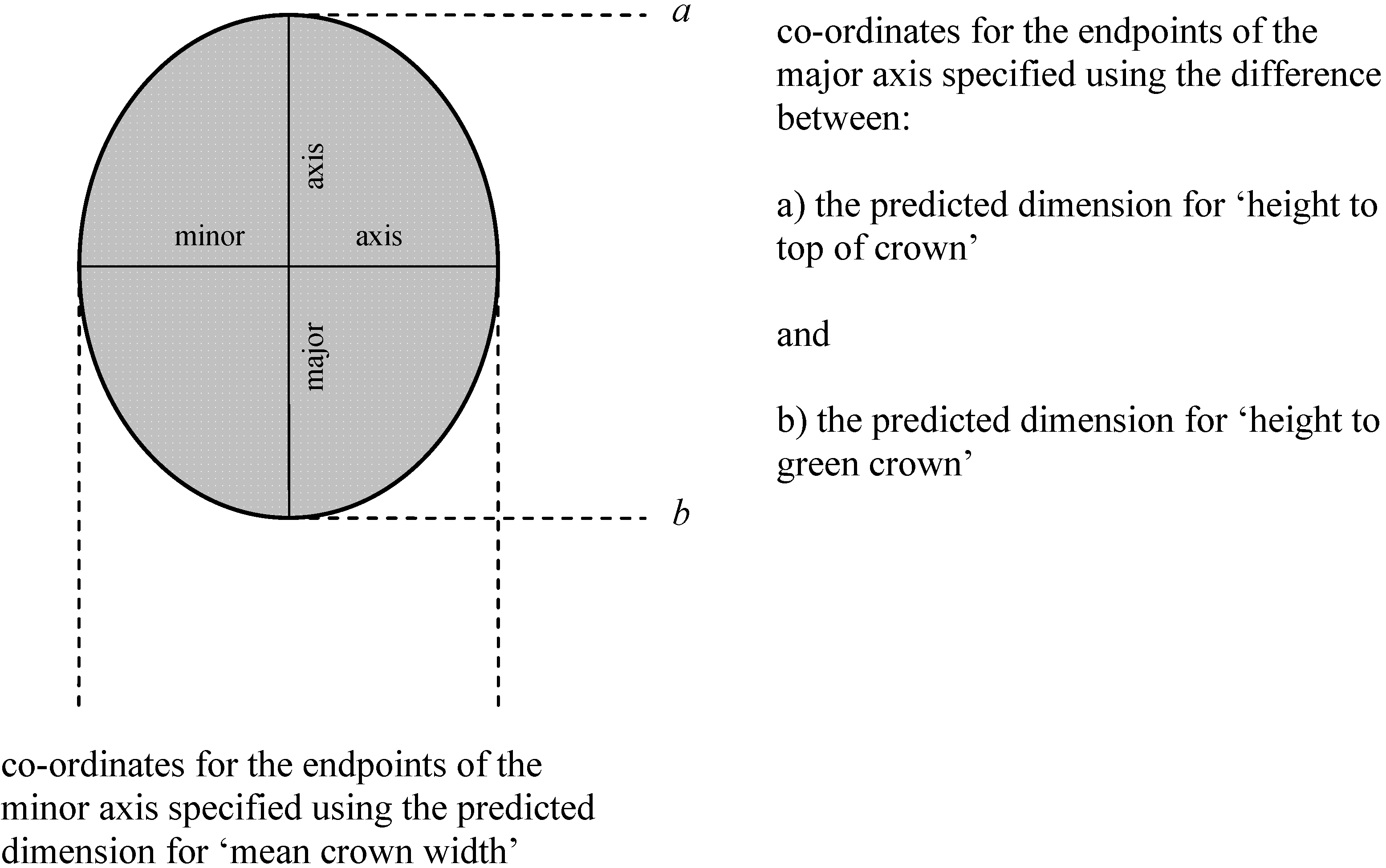
Canopy spatial models were constructed using AutoCAD™ architectural software (AutoCAD 2000 Copyright 1982-2000 AutoDesk Inc.). Crown profiles for each genus were reproduced in AutoCAD™ based on the selection of an appropriate regular geometric figure(s). Crown profiles have been used in a number of similar studies [
28,
38] and were considered to be suitable for model construction. The dimensions of a given crown profile were predicted using modelled relationships between dbh and height to top of crown, height to base of green crown and mean crown width (
Figure 1). If a crown profile consisted of more than one figure, then changes that might occur in the relative shape and size of each figure as dbh increased were also incorporated into the model.
Figure 1.
Specifying the dimensions of an elliptical crown profile in AutoCAD™. Dimensions were predicted using allometrics relating height to top of crown, height to base of green crown and crown width respectively to dbh.
Figure 1.
Specifying the dimensions of an elliptical crown profile in AutoCAD™. Dimensions were predicted using allometrics relating height to top of crown, height to base of green crown and crown width respectively to dbh.
A series of crown profiles was generated for each genus based on the respective crown measurements at the midpoints of 5 cm wide dbh classes. A corresponding crown solid was then generated for each profile of each genus by revolving a given profile around its vertical axis. Crown solids representing senescent eucalypts outside the domain of the regression equations were specified directly from field measurements.
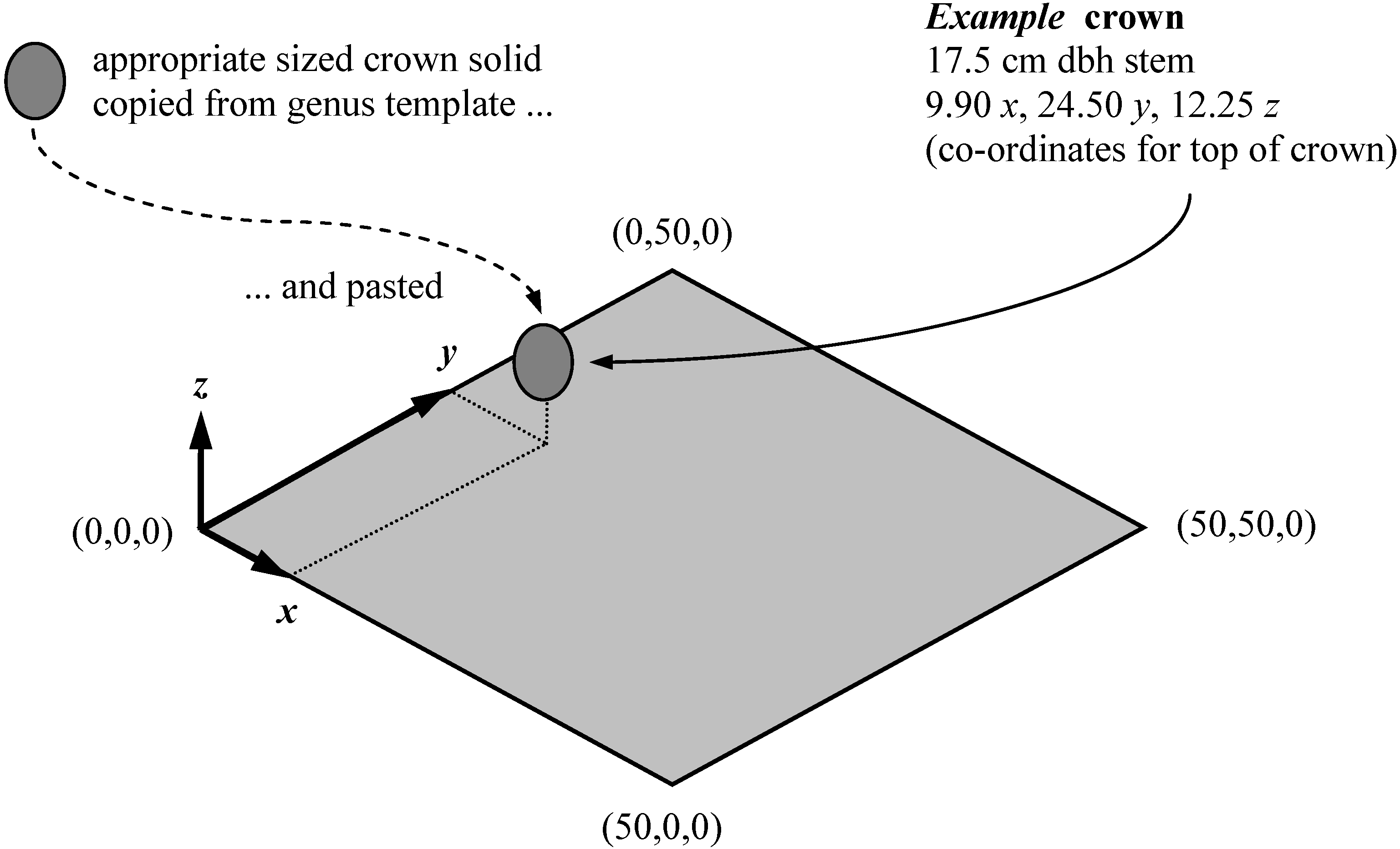
A three-dimensional canopy model was then assembled for each of the four plots. Each canopy model was ‘populated’ with the appropriate crown solids to match each corresponding real crown. This was accomplished using the plot data describing the genus, dbh and relative location of each stem > 10 cm dbh (
Figure 2). All modelled crowns were assumed to be directly above their respective stems and the
z co-ordinates for the top of the crown solids were calculated using the relevant regression equation for ‘height to top of crown’. Eucalypt crown solids were classified as healthy, suppressed or senescent in accordance with field observations.
A set of simple rules was used to model the competitive interaction between overlapping crowns. Crowns of the same genus were considered to share overlapping space equally. For crowns of different genera the overlapping volume was allocated to the more shade-tolerant genus. Based on the work of Read (39) on the photosynthetic and growth responses of the major canopy species within Tasmania’s cool temperate rainforests,
Atherosperma was modelled as more shade-tolerant than
Nothofagus. Similarly, based on the work of Cunningham and Cremer (40) on the regeneration characteristics of the understorey vegetation within wet eucalypt forests, these ‘climax’ rainforest genera were modelled as more shade-tolerant than faster growing, ‘pioneer’ understorey genera such as
Nematolepis or
Pomaderris. Otherwise, there were only rare instances of overlap between the crowns of other combinations of genera, or in the case of
Eucalyptus, categories of crown condition. In such instances, if the crown solid of a ‘healthy’
Eucalyptus overlapped the crown solid of either a ‘suppressed’ or ‘senescent’
Eucalyptus, the shared volume was allocated to the healthy crown; and if an
Acacia crown solid overlapped the crown solid of either a ‘suppressed’ or ‘senescent’
Eucalyptus, the shared volume was allocated to the
Acacia crown. Portions of crown solids that protruded beyond the modelled plot boundaries were deleted from the canopy models, which were then horizontally partitioned at intervals of 2 m to investigate canopy stratification (
Figure 3).
Figure 2.
An example of populating a canopy model with a crown solid copied from a genus template and pasted to the appropriate spatial position relative to the plot origin (distances in metres). This operation was repeated for each crown within the study plots.
Figure 2.
An example of populating a canopy model with a crown solid copied from a genus template and pasted to the appropriate spatial position relative to the plot origin (distances in metres). This operation was repeated for each crown within the study plots.
The volume of the modelled crown solids was obtained from the canopy models for each genus within 2 metre height classes to a lower limit of 8 m using the relevant command within AutoCAD™. Height classes <8 m were excluded because they were dominated by the crowns of trees and shrubs <10 cm dbh. A ‘foliage density factor’ was applied to the volume data for each genus, and in the case of Eucalyptus, to the different categories of crown condition. These factors reduced or increased the modelled density of foliage for each genus, and in the absence of published data, were based on a subjective appraisal of the density of foliage within the crowns of the trees at the study plots. Further work is being undertaken to refine this aspect of the methodology, however we consider the preliminary results of this subjective appraisal to be more realistic than to have modelled crowns as if they were equivalent in foliage density. Vertical canopy profiles were then constructed to summarise the distribution of foliage amongst different genera and height strata for the four study sites. These profiles were used to delineate distinct canopy strata and to identify the genera occupying each stratum.
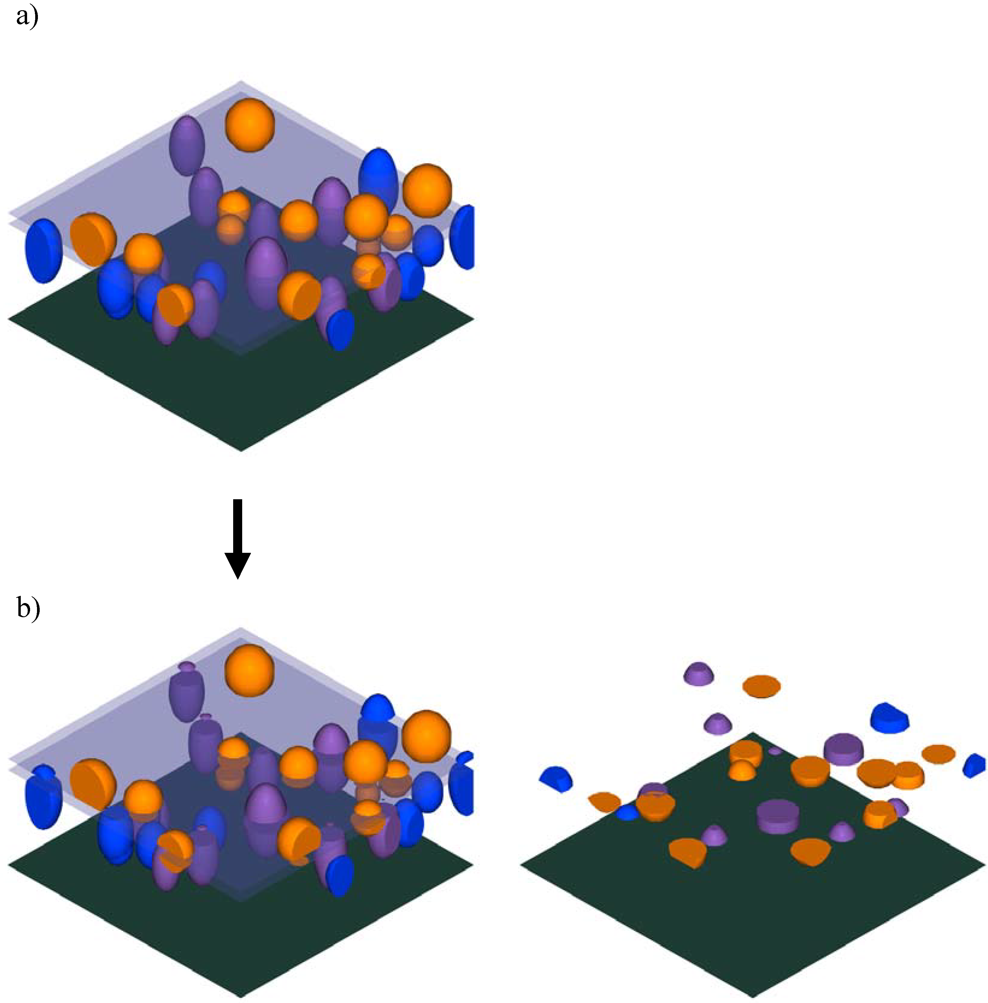
Figure 3.
Horizontally slicing the canopy model of a hypothetical plot: a) the original canopy model showing two slicing planes spaced at a 2 m interval; b) the canopy model after the completion of one slicing operation, showing the portions of crown solids within that height class removed from the model (left) for easier display (right). This operation was repeated for each successive interval to fully investigate stratification within the canopy.
3. Results
Six canopy genera were identified on the basis of their contribution to the basal area of the plots (
Table 2). Quadratic functions were used to model crown dimensions for each of the six genera, unless the second degree term was not significant (p > 0.05), in which case a linear function was used (
Table 3). Models were fitted with JMP™ statistical software (JMP™ Version 7.0 Copyright 1989-2007 SAS Institute Inc.). The distributions of the residuals for all crown dimension models were approximately normal, with little or no heteroskedasticity. For
Nematolepis, the limited size and range of the stems available for sampling precluded the determination of the relationships between ‘height to top of crown’ and dbh, and ‘height to green crown’ and dbh. Instead the mean values for these dimensions were used in the spatial models.
Table 2.
Proportion (%) of plot basal area occupied by each genusa. Shaded rows indicate genera which contributed >1% of plot basal area (remaining genera were excluded from canopy models).
Table 2.
Proportion (%) of plot basal area occupied by each genusa. Shaded rows indicate genera which contributed >1% of plot basal area (remaining genera were excluded from canopy models).
| | plot |
| genus | 1966S | 1934S | 1898S | OGS |
| Acacia | 0.7 | 3.7 | 13.5 | 4.9 |
| Atherosperma | − | 2.2 | 1.7 | 15.8 |
| Eucalyptus | 93.1 | 87.1 | 62.8 | 54.9 |
| Eucryphia | 0.1 | 0.4 | − | − |
| Leptospermum | − | < 0.1 | − | − |
| Monotoca | − | 0.6 | − | − |
| Nematolepis | 4.6 | 0.2 | − | − |
| Nothofagus | − | 5.5 | 1.0 | 24.2 |
| Olearia | − | − | 0.1 | − |
| Pomaderris | 1.5 | − | 20.8 | − |
| Phyllocladus | − | 0.2 | − | < 0.1 |
| Tasmannia | − | 0.1 | − | − |
Three large senescent Eucalyptus were excluded from the regression analysis as outliers, since the condition of their crowns was related to stochastic processes (e.g., internal rot, wind damage) rather than to a continuing strong allometric relationship between their crown dimensions and their stem diameter at breast height. Crowns of these three trees, and one additional senescent Eucalyptus were recreated in the canopy models based on direct field measurements.
Table 3.
Equations to predict crown dimensionsa (m) in terms of dbh (cm) for the modelled genera.
Table 3.
Equations to predict crown dimensionsa (m) in terms of dbh (cm) for the modelled genera.
| genus | crown dimension regression equation | R2 | p value |
| Acacia | T | = 13.006 + 0.387dbh | 0.75 | <0.0001 |
| | B | = 11.175 + 0.199dbh | 0.25 | 0.0002 |
| | W | = 1.996 + 0.154dbh | 0.73 | <0.0001 |
| Atherosperma | T | = 10.036 + 0.437dbh − 0.007(dbh − 23.714)2 | 0.55 | <0.0001 |
| | B | = 6.952 + 0.101dbh | 0.05 | 0.0456 |
| | W | = 4.156 + 0.069dbh | 0.24 | 0.0037 |
| Eucalyptus | T | = 15.868 + 0.411dbh − 0.003(dbh − 53.346)2 | 0.76 | <0.0001 |
| | B | = 13.622 + 0.255dbh − 0.002(dbh − 53.346)2 | 0.54 | <0.0001 |
| | W | = 1.966 + 0.115dbh | 0.85 | <0.0001 |
| Nematolepis | T | = 12.25 m | − | NSb |
| | B | = 5.7 m | − | NS |
| | W | = 0.680 + 0.210dbh | 0.41 | 0.0477 |
| Nothofagus | T | = 11.574 + 0.428dbh − 0.007(dbh − 26.156)2 | 0.65 | <0.0001 |
| | B | = 5.895 + 0.150dbh | 0.18 | <0.0001 |
| | W | = 2.66 + 0.135dbh − 0.002(dbh − 26.156)2 | 0.61 | <0.0001 |
| Pomaderris | T | = 9.207 + 0.577dbh − 0.042 (dbh − 14.570)2 | 0.45 | <0.0001 |
| | B | = 7.100 + 0.374dbh | 0.24 | <0.0001 |
| | W | = 0.483 + 0.192dbh | 0.55 | <0.0001 |
Crown profiles for
Acacia,
Atherosperma,
Nematolepis,
Nothofagus and
Pomaderris were modelled as single ellipses. Crown profiles for
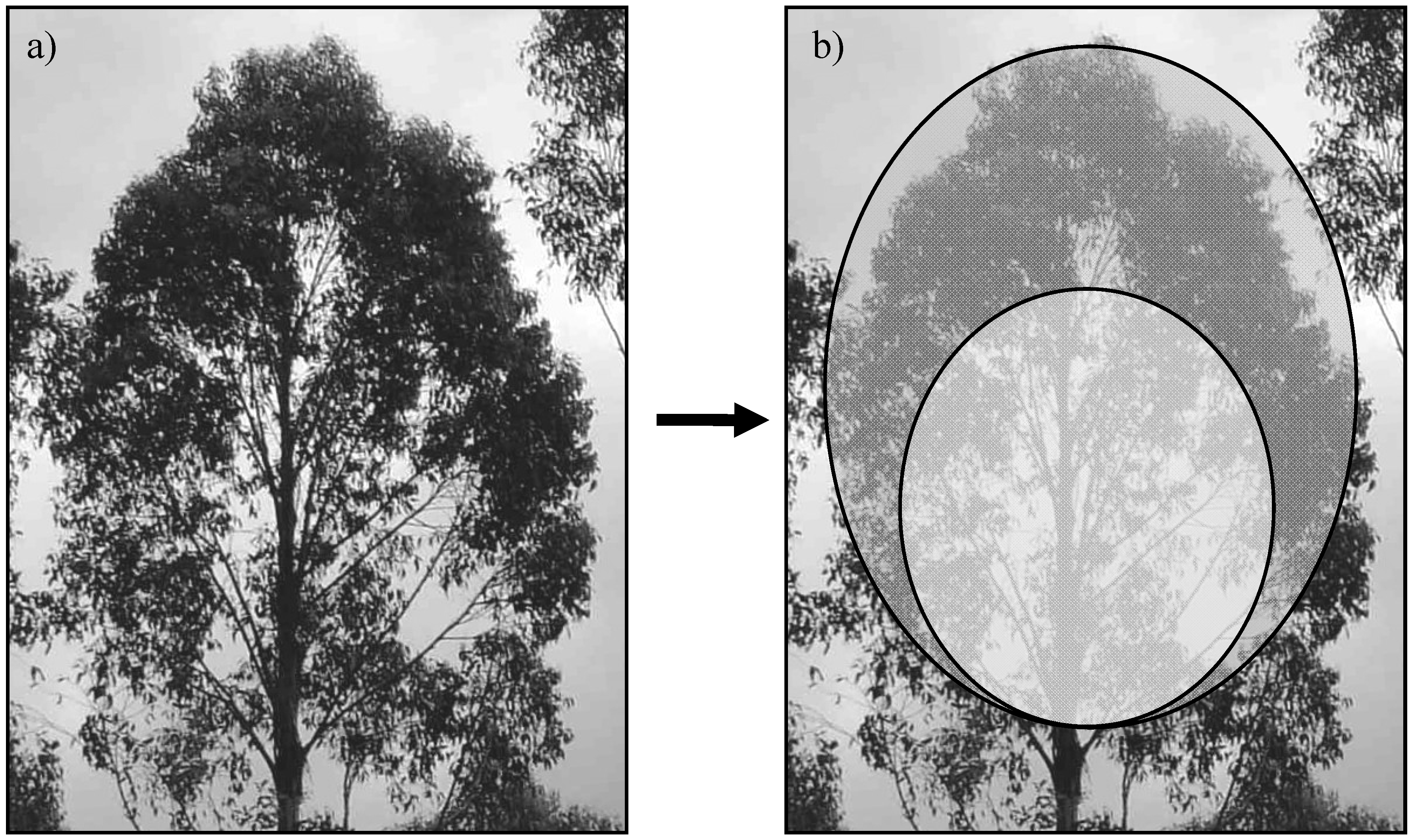
Eucalyptus were initially modelled as overlapping ‘paired’ ellipses to delineate zones of different foliage density within their crowns, based on the results of photographs and field observation (e.g.,
Figure 4 and
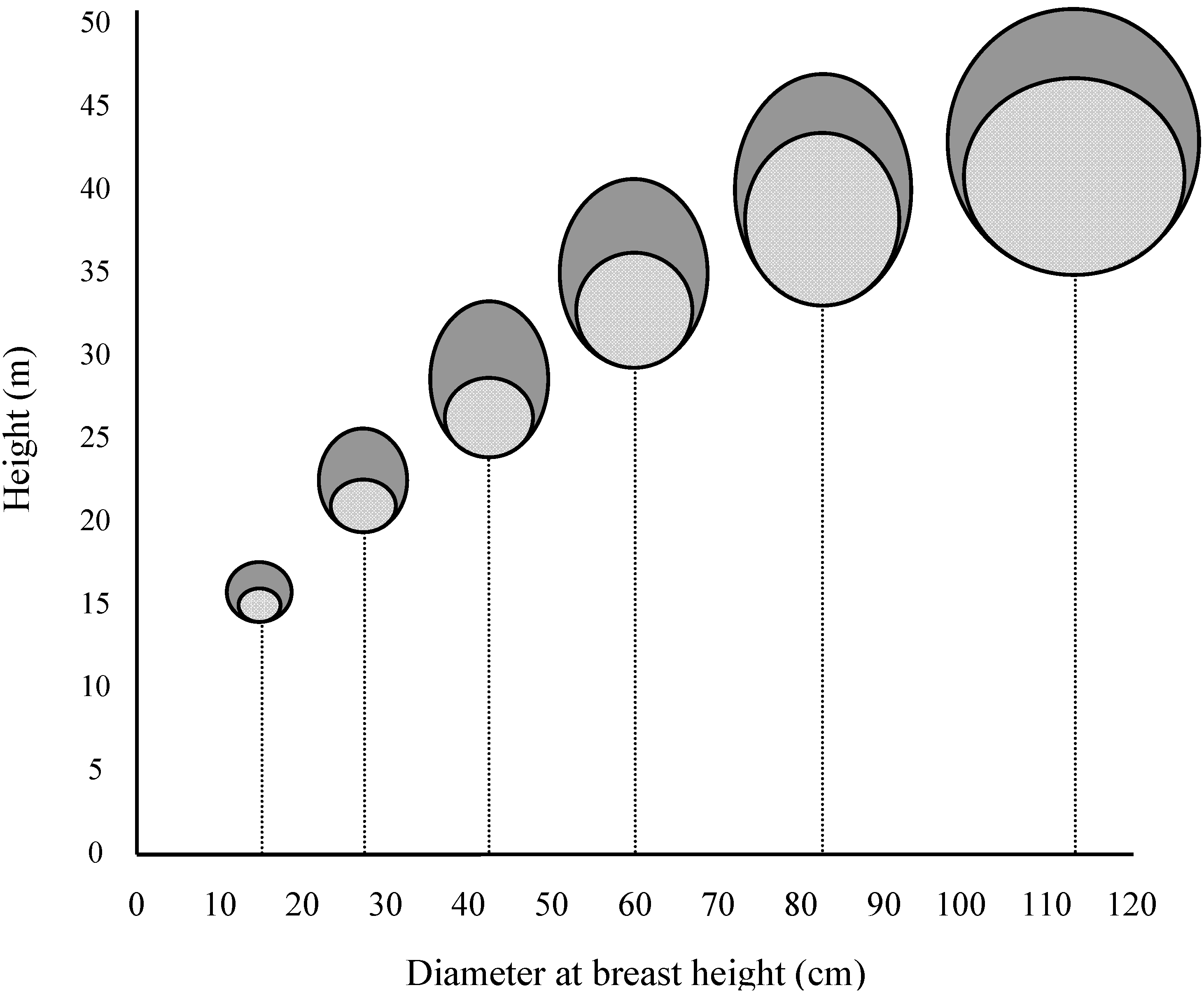
Figure 5). The larger ellipse of each pair was then reduced to a crescent shaped profile. Representative changes in the relative size and shape of each pair (related to the expansion of the crown with increasing dbh) are presented in
Figure 6. The crown profiles were used to create crown solids for each genus, which then served as the ‘templates’ for populating the canopy models. The completed canopy models for each plot are shown in plan view (
Figure 7) and in southeast isometric view (
Figure 8).
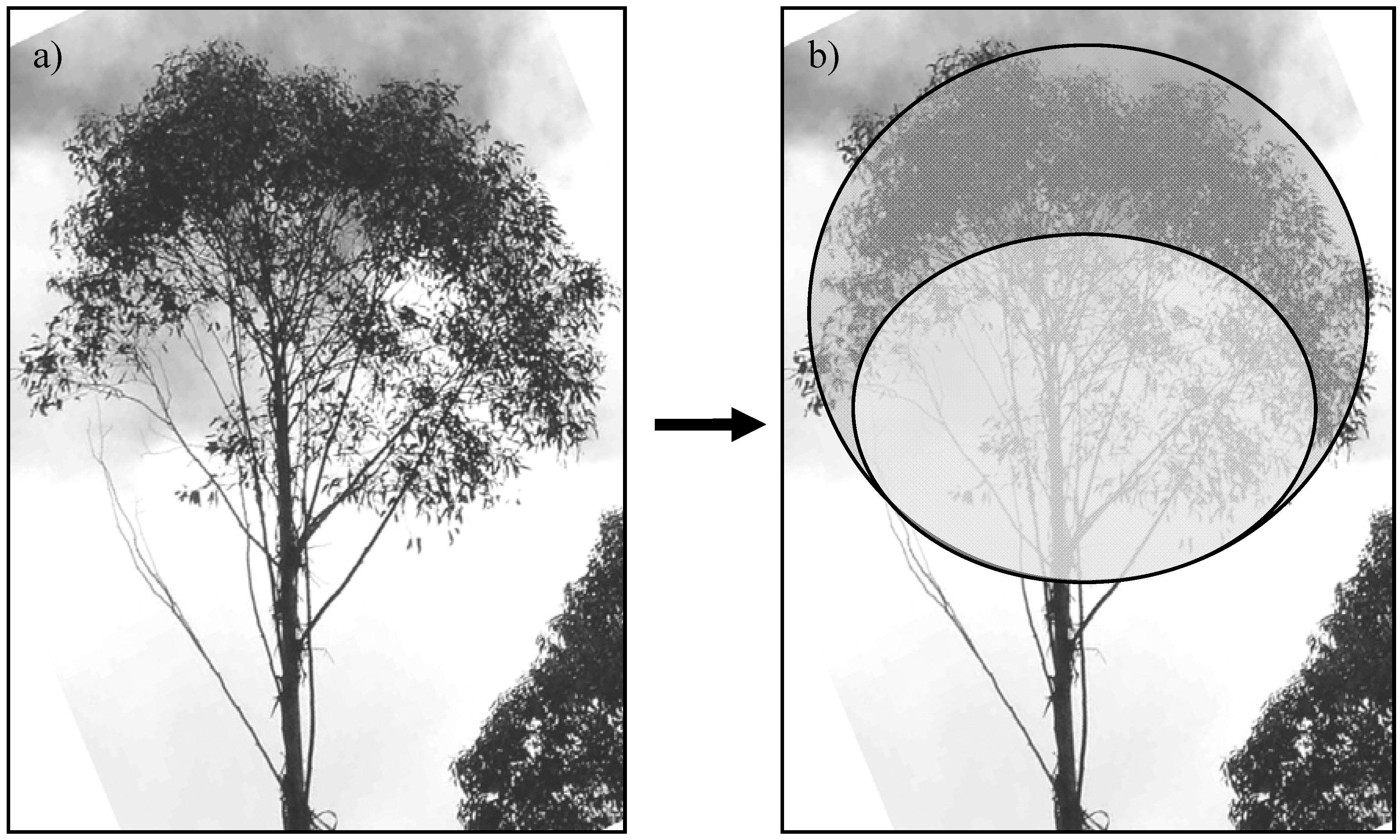
Figure 4.
An example of a crown profile used for Eucalyptus crowns: a) the crown of a smaller dbh Eucalyptus in a thinned coupe adjacent to the 1966S plot represented by b) an ellipse of ‘sparser foliage’ superimposed on a second ellipse of ‘denser foliage’.
Figure 4.
An example of a crown profile used for Eucalyptus crowns: a) the crown of a smaller dbh Eucalyptus in a thinned coupe adjacent to the 1966S plot represented by b) an ellipse of ‘sparser foliage’ superimposed on a second ellipse of ‘denser foliage’.
Figure 5.
A second example of a crown profile used for Eucalyptus crowns: a) the crown of a larger dbh Eucalyptus in a thinned coupe adjacent to the 1966S plot represented by b) an ellipse of ‘sparser foliage’ superimposed on a second ellipse of ‘denser foliage’.
Figure 5.
A second example of a crown profile used for Eucalyptus crowns: a) the crown of a larger dbh Eucalyptus in a thinned coupe adjacent to the 1966S plot represented by b) an ellipse of ‘sparser foliage’ superimposed on a second ellipse of ‘denser foliage’.
Figure 6.
Crown profiles for Eucalyptus were initially modelled as overlapping ‘paired’ ellipses to delineate zones of different foliage density within their crowns. The larger ellipse of each pair has been reduced to a crescent shape.
Figure 6.
Crown profiles for Eucalyptus were initially modelled as overlapping ‘paired’ ellipses to delineate zones of different foliage density within their crowns. The larger ellipse of each pair has been reduced to a crescent shape.
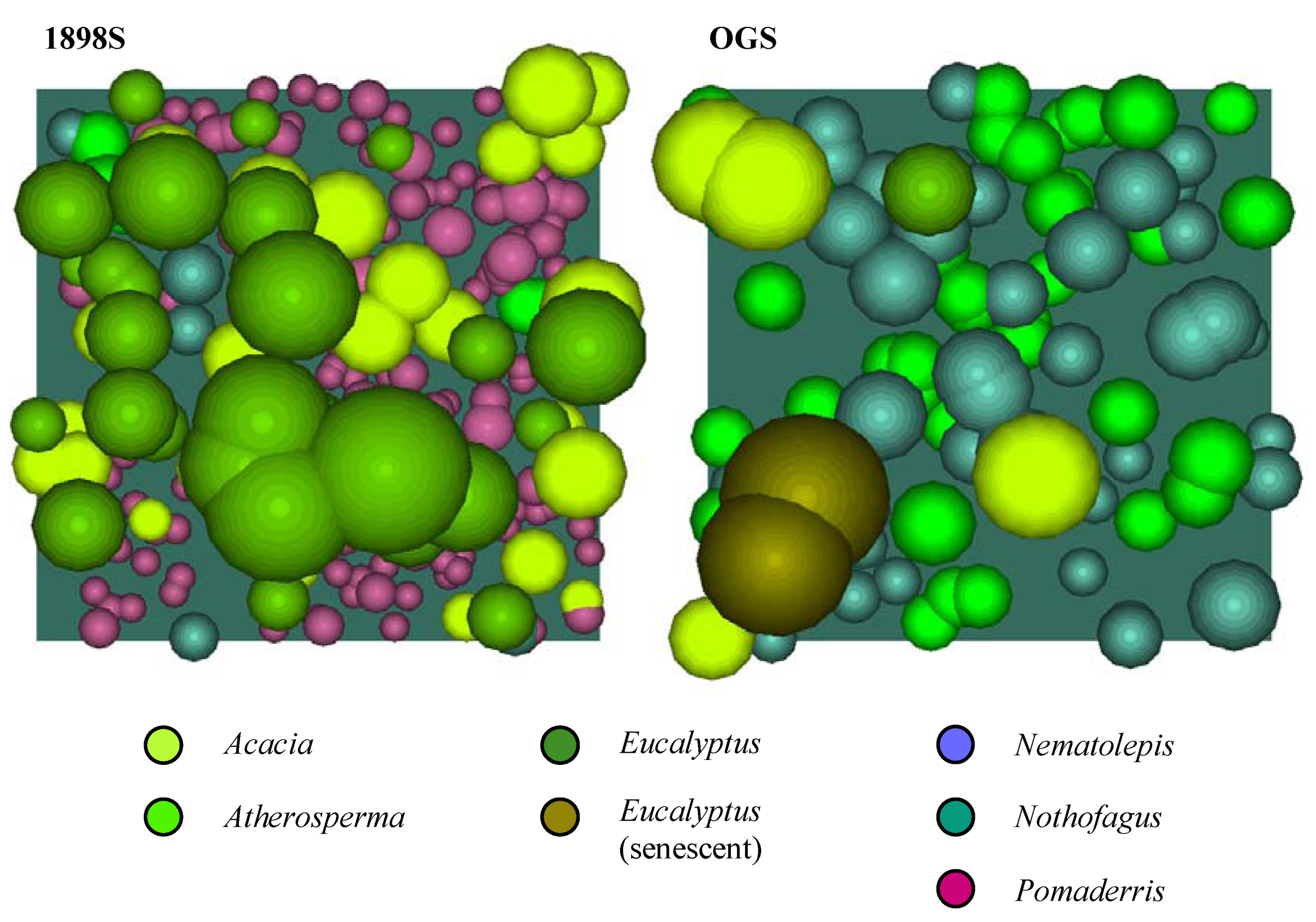
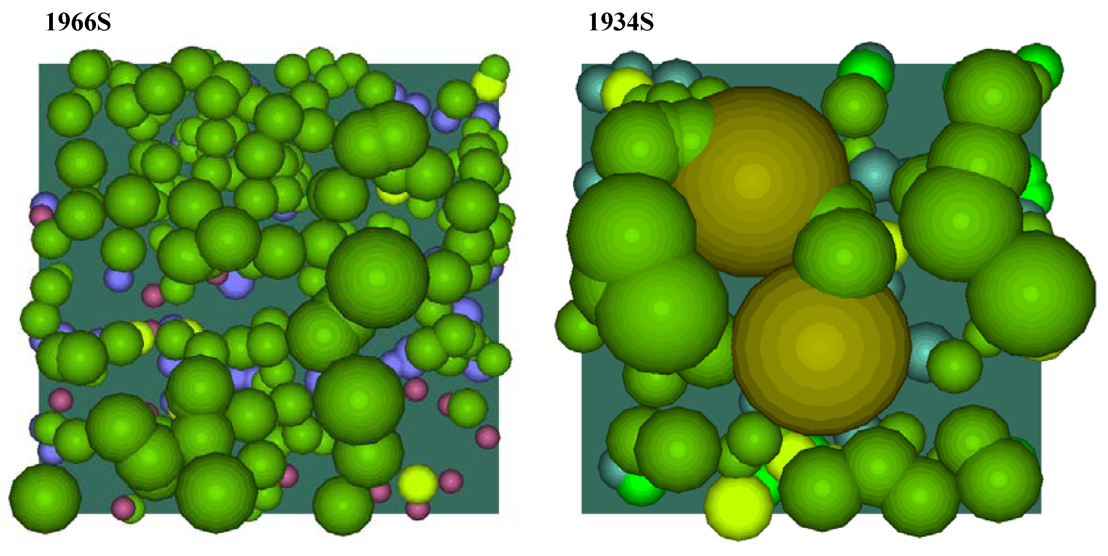
Figure 7.
The completed canopy models for each plot (plan view).
Figure 7.
The completed canopy models for each plot (plan view).
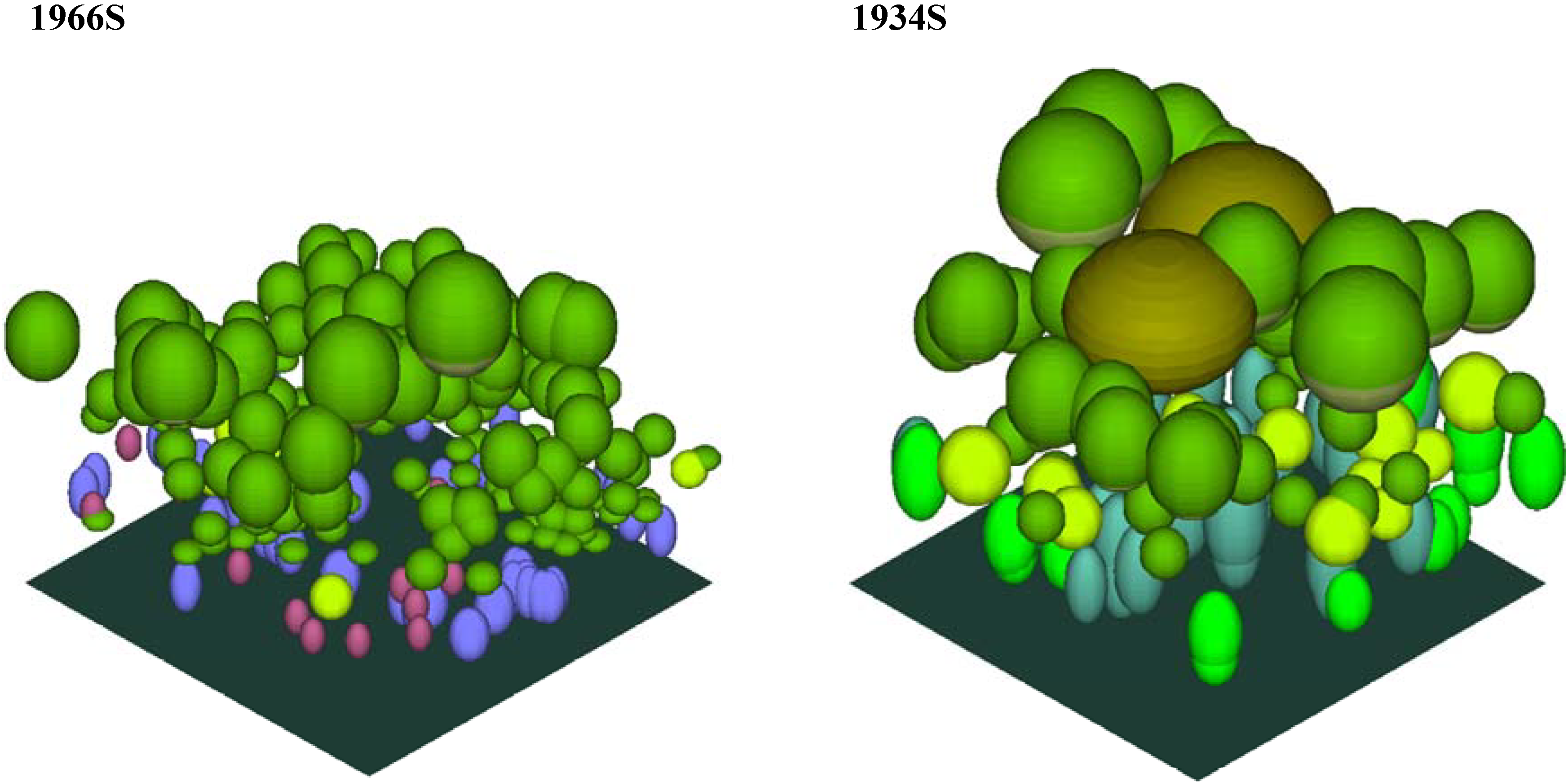
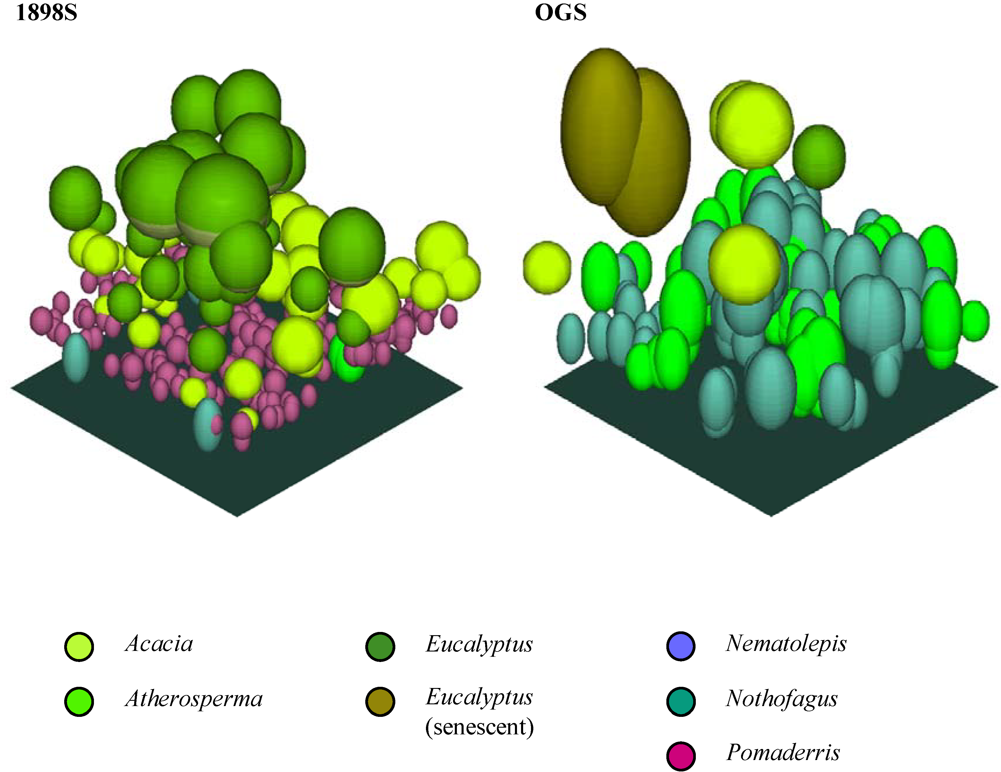
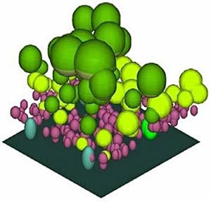
Figure 8.
The completed canopy models for each plot (southeast isometric view).
Figure 8.
The completed canopy models for each plot (southeast isometric view).
To more accurately represent the foliage volumes of crowns, a ‘foliage density factor’ was applied to the crown solids of different genera, and in the case of
Eucalyptus, to the crown solids representing different categories of crown condition (
Table 4). A density factor of 1 was assigned to the crowns of
Acacia,
Nematolepis and
Pomaderris; based on a subjective appraisal of equivalent densities of foliage within their crowns. A density factor of 1.2 was assigned (representing a 20% increase in foliage density) to the crowns of the more shade-tolerant genera,
Atherosperma and
Nothofagus; and a density factor of 0.8 (representing a 20% decrease in foliage density) to the crowns of shade-intolerant
Eucalyptus. The crowns of senescent and suppressed
Eucalyptus were further reduced by 50% to a density factor of 0.4; and the sparsely-foliated interior volumes of healthy and suppressed
Eucalyptus crowns were estimated as having 25% of the foliage density of their more densely-foliated outer shells (
i.e., density factors of 0.2 and 0.1, respectively).
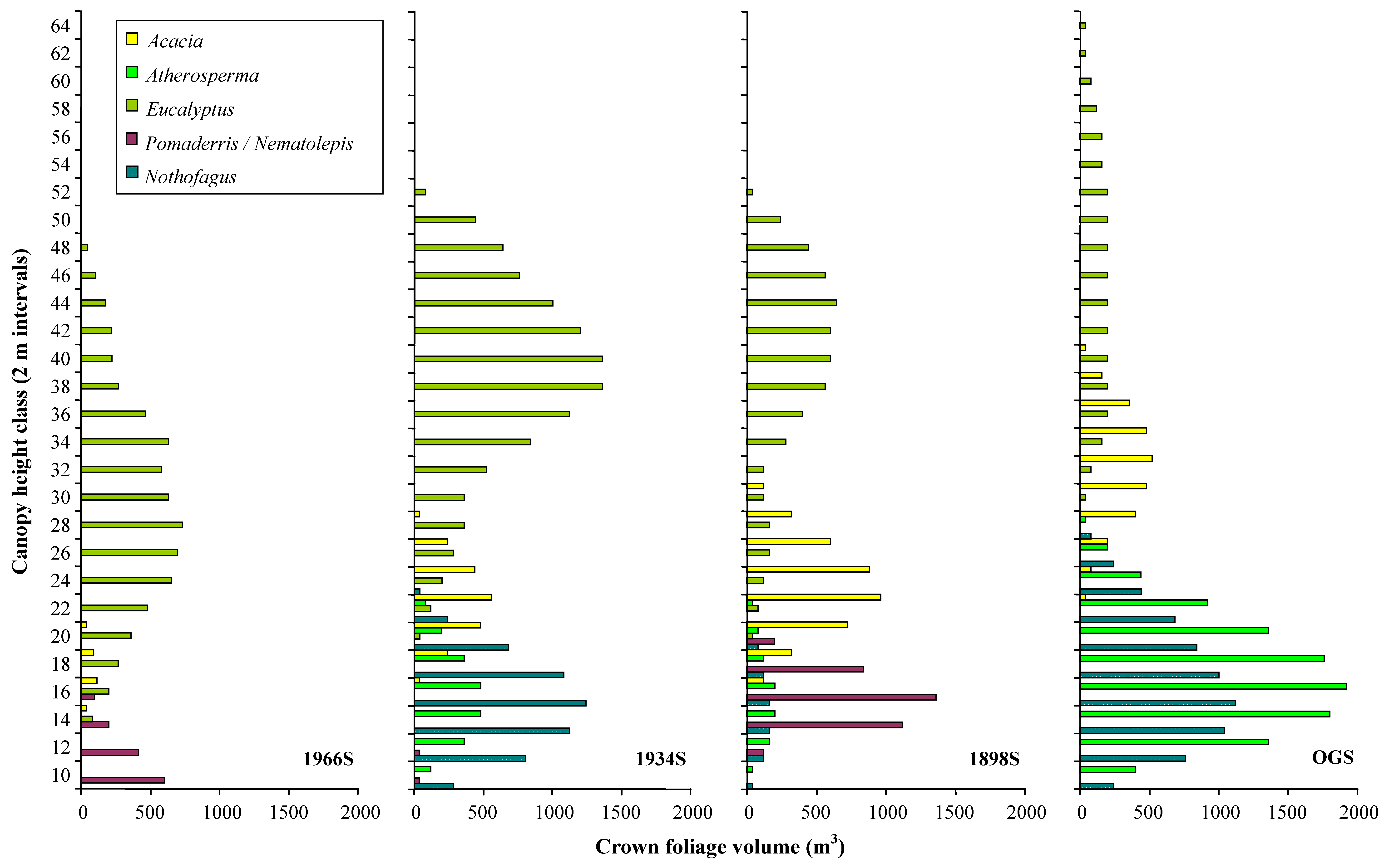
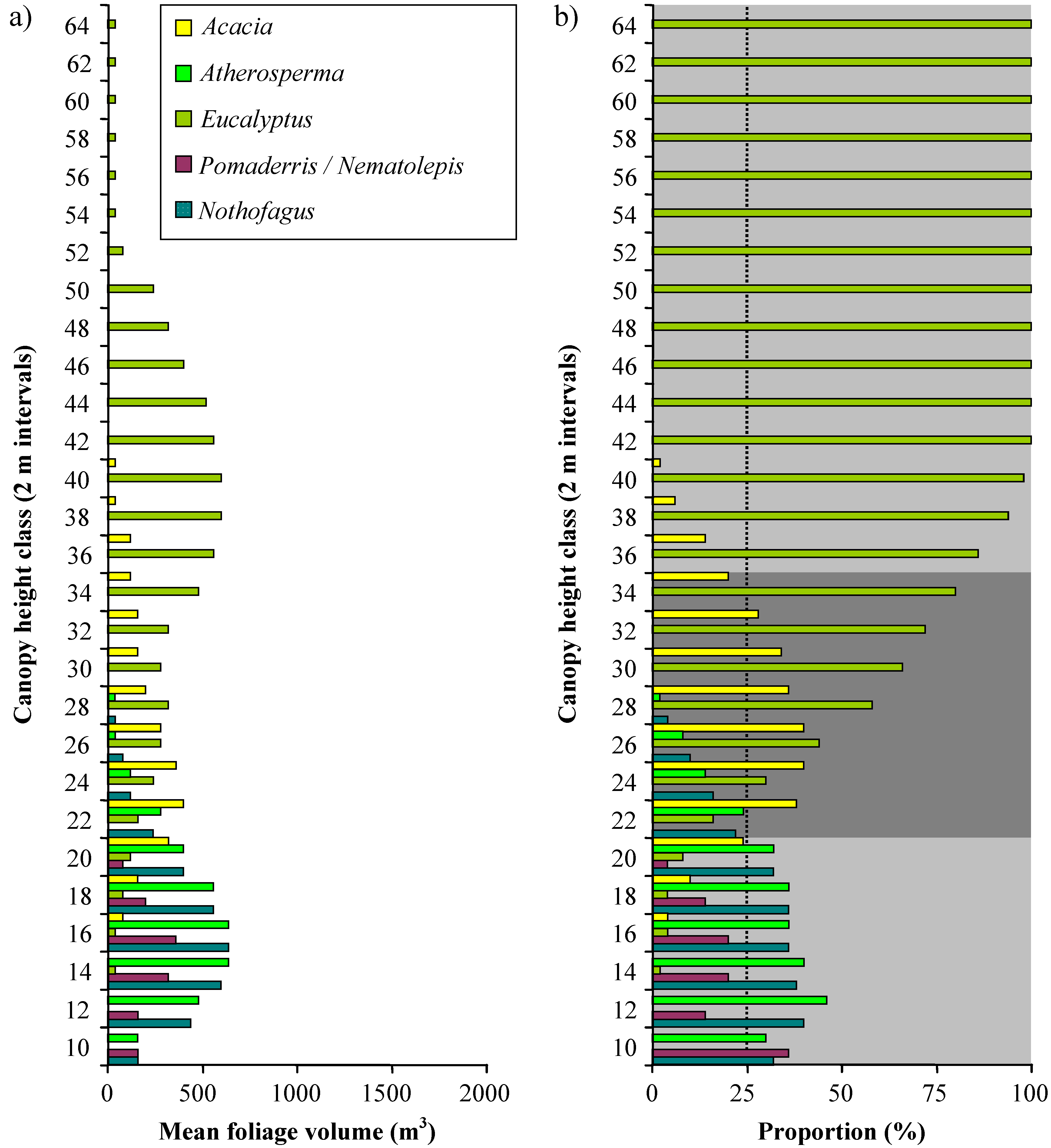
Vertical profiles of the distribution of foliage volume in 2 m height classes are shown in
Figure 9. The mean distribution of foliage volume across all four plots is shown in
Figure 10a and as proportions of the total volume in each height class in
Figure 10b. The results for the five types of crown solid used to model
Eucalyptus were aggregated for ease of comparison with other genera. The results for
Nematolepis and
Pomaderris were also aggregated since both genera are typical of the understorey of wet sclerophyll forest, and can be considered interchangeable in that respect.
Eucalyptus was the dominant genus in the upper part of the canopy at every plot; accounting for more than 50% of the mean foliage volume above 26 m in height, and 100% of the mean foliage volume above 40 m in height. Total volume reaches a peak at the 1934S plot and declines thereafter.
Acacia dominated the middle layers of the modelled canopies, accounting for more than 25% of the mean foliage volume between 20 and 32 m in height.
Nematolepis and
Pomaderris dominated the lower layers of the 1966S and 1898S plots; but were only a minor component of the structure at the 1934S plot, and entirely absent from the OGS plot. It was only in the lowest height class (8-10 m) that these genera accounted for more than 25% of the mean foliage volume. In contrast to
Nematolepis and
Pomaderris,
Atherosperma and
Nothofagus dominated the lower layers of the 1934S and OGS plots; but were only a minor component of the structure at the 1898S plot, and entirely absent from the 1966S plot. Across all plots
Atherosperma and
Nothofagus contributed more than 25% of mean foliage volume between 8 and 20 m.
Table 4.
Density factors used to modify the volume of foliage within modelled crowns of different genera and eucalypts of different crown condition.
Table 4.
Density factors used to modify the volume of foliage within modelled crowns of different genera and eucalypts of different crown condition.
| Genus | Modelled crown solid type | Density factor |
| Atherosperma | all crowns | 1.2 |
| Acacia | all crowns | 1.0 |
| Eucalyptus | outer shell, healthy crown | 0.8 |
| Eucalyptus | inner volume, healthy crown | 0.2 |
| Eucalyptus | outer shell, suppressed crown | 0.4 |
| Eucalyptus | inner volume, suppressed crown | 0.1 |
| Eucalyptus | senescent crown | 0.4 |
| Nematolepis | all crowns | 1.0 |
| Nothofagus | all crowns | 1.2 |
| Pomaderris | all crowns | 1.0 |
These results indicate the presence of three distinct strata at the plots (
Figure 10b). At heights above 34 m, the canopy is dominated by
Eucalyptus; between 20 and 34 m, the canopy is dominated by
Eucalyptus and
Acacia; and between 8 and 20 m the canopy is dominated by rainforest genera (
Atherosperma and
Nothofagus), with a substantial presence of wet sclerophyll forest understorey genera (
Nematolepis and
Pomaderris).
Figure 9.
Crown foliage volumes × height class × genus for the four canopy models. Height values are upper thresholds for each 2 m interval.
Figure 9.
Crown foliage volumes × height class × genus for the four canopy models. Height values are upper thresholds for each 2 m interval.
Figure 10.
a) Distribution of mean foliage volume in all four plots combined amongst height classes and canopy genera. b) Distribution of the proportion of mean foliage volume within each height class amongst different genera. A 25% threshold (dotted line) was used to identify genera that dominate distinct canopy strata. The three identified strata are shown as shaded bands.
4. Discussion
Our methodology provides a relatively rapid means of modelling complex canopy structures such as those in the tall wet eucalypt forests of southern Tasmania. Our results confirmed our initial hypotheses. We successfully predicted the geometry of free-growing crowns on the basis of dbh. Not surprisingly, the relationships for predicting ‘height to top of crown’ in terms of dbh were stronger than those for predicting ‘height to green crown’ for all genera and the relationships to predict crown dimensions were stronger for shade-intolerant genera (Eucalyptus and Acacia) than shade-tolerant genera (Atherosperma and Nothofagus). Although no single modelled crown can be expected to exactly represent its real world counterpart, we consider these relationships to be suitable for modelling the canopy at the plot or stand level. Spatial models of the canopy structure at each study plot were created with AutoCAD™ using the field data describing the genus, dbh and relative positions of all trees greater than 10 cm dbh and observations of the typical crown shape for each genus. The problem of modelling tree crowns as free-growing within closed growing conditions was addressed by using AutoCAD™ to model the effects of competition for light between neighbouring trees to more accurately represent these conditions. By horizontally partitioning the resulting canopy models, it was possible to identify the presence of distinct strata in stands of different ages, and to identify the dominant genera associated with each.
A number of other studies have modelled canopy structure using computer-aided design (CAD) software [
41,
42,
31], or GIS software [
28,
29] to integrate data describing the location and dimensions of individual tree crowns. A drawback to the techniques used in many of these studies is the amount of time required to measure crowns individually in the field, particularly in closed forest conditions. For example Van Pelt and Franklin [
30] explicitly modelled the vertical and horizontal distribution of individual crowns, and made only minimal use of regression equations to predict crown dimensions. While their estimates of individual crown size and shape are no doubt highly accurate, they acknowledge the help of “more than 50 people who assisted with various aspects of the fieldwork, which took the better part of five field seasons to collect” [
30]. Silbernagel and Moeur [
31] avoided much of this effort by using previously developed regression equations to predict crown size and shape, as was done in our study. However the questions of ‘competition between crowns’ and the realistic estimation of individual crown volumes never arose because the focus of their study was the
gaps between adjacent crowns rather than the crowns themselves.
In contrast to these studies our methodology provides a comparatively quick and inexpensive means of modelling canopy structure, that should be applicable to a range of forest and woodland communities providing the necessary regression equations and competition rules are developed for the community concerned. The method could therefore provide a practical means of quantifying canopy structure across a broad range of study sites to provide data for ground truthing remote sensing technologies. In particular LiDAR offers great potential for characterising vertical structure, but its use is currently hampered by difficulties associated with interpreting signals returned from the interior of the canopy [
15,
43]. This problem is exacerbated when the number of these ‘returns’ is reduced by a high density of foliage at the top of the canopy, and especially in closed forests where there is limited penetration [
16]. The methodology described here could aid the interpretation of these returns by providing a more rigorous foundation for identifying where strata begin and end, as well as helping to determine which genera dominate particular strata. If the vertical extents and characteristic genera for a stratum are known, then any returns between these extents could be aggregated and attributed to those genera with greater confidence.
The ability to map the
existing canopy structure using the methodology presented here (either directly or in conjunction with remote-sensing technologies) would be an improvement on trying to
predict canopy structure based on the effects of past disturbances. Much of the diversity in the structure of forest canopies is acknowledged to be strongly influenced by the disturbance history of a particular stand, and in particular the highly variable effects of fire [
44,
45]. Reconstructing the disturbance history of a forest is possible to some extent [
46,
36], but
predicting the effects of a particular disturbance regime on forest structure remains highly problematic [
47,
48,
7]. Many of these problems could be avoided by directly quantifying canopy structure. The methodology presented here is a useful step towards developing an efficient and reliable research tool for this purpose.

