Structural Damage Localization by the Principal Eigenvector of Modal Flexibility Change

Abstract

Using the principal eigenvector (PE) of modal flexibility change, a new vibration-based algorithm for structural defect localization was presented in this paper. From theoretical investigations, it was proven that the PE of modal flexibility variation has a turning point with a sharp peak in its curvature at the damage location. A three-span continuous beam was used as an example to illustrate the feasibility and superiority of the proposed PE algorithm for damage localization. Furthermore, defect localization was also performed using the well-known uniform load surface approach for comparison. Numerical results demonstrated that the PE algorithm can locate structural defects with good accuracy, whereas the ULS approach occasionally missed one or two defect locations. It was found that the PE algorithm may be promising for structural defect assessment.

1. Introduction

During the last decades, a large number of research papers have reported on structural defect assessment based on the changes in measured static/dynamic response. The theoretical basis of these algorithms lies in the fact that the static and dynamic responses are functions of structural material properties (such as stiffness, mass, and damping). As a result, if the material properties are changed due to structural defects, then structural responses must also be changed. The relevant literature reviews can be found in references [1,2,3]. Generally, defect identification algorithms can be divided into model based and non-model based procedures according to using finite element model (FEM) or not. Algorithms [4,5,6,7,8,9,10,11,12,13,14,15,16] based on FEM assess structural defects by modifying structural FEM according to structural responses. The modifications of structural FEM will indicate the location and severity of the defect. It is well known that model-based methods are computationally intensive and highly influenced by the quality of structural FEM. However, the precise FEM is often difficult to achieve in engineering practice for the simplified assumptions in the construction of the FEM, which means that the correct results might be missed.

The advantages of non-model algorithms lie in their easiness and straightforwardness because structural EEMs are not needed in these approaches. Damage indexes can be established directly by the variations of structural responses before and after damage for assessing structural defects. Zhang and Aktan [17] used the uniform load surface (ULS) of structural flexibility to locate defects. Wu and Law [18,19] discovered that the curvature of ULS is sensitive to local damage in the plate structure. Wang and Qiao [20] made use of the simplified gapped-smoothing technique to improve the accuracy of the ULS algorithm. Choi et al. [21] proposed an elastic damage load theorem to locate defects in simply supported beams. Sung et al. [22] presented a normalized ULS algorithm for damage identification in beam-like structures. Other algorithms for defect localization can be found in references [23,24,25,26,27]. In engineering practice, structural response parameters are sometimes difficult to obtain and/or depend on environmental factors (e.g., temperature, humidity, loading at the time of testing, etc.). If the environmental impact is not considered properly, these localization algorithms will probably give incorrect results. In view of this, Limongelli et al. [9,28,29] proposed the interpolation damage detection method (IDDM) to considering the environmental impact. Their investigations verified the effectivity of the IDDM. Manoach et al. [30,31] proposed a new damage index and a method based on the Poincare map for structural damage localization. Numerical and experimental studies confirm the applicability and sensitivity of their method in application.

This study proposes a defect localization algorithm based on the principal eigenvector (PE) obtained from structural flexibility variation. The presented algorithm uses PE as a new damage indicator to locate structural defects without FEM. A three-span continuous beam is used as an example to demonstrate the efficiency of the presented PE algorithm in structural defect localization. For several damage scenarios in the structure, defect localization results obtained by the PE algorithm and the ULS procedure are both given for comparison. The numerical result demonstrated that the PE algorithm can locate structural defects with good accuracy, whereas the ULS approach occasionally missed one or two defect locations. It has been shown that the proposed PE algorithm may be more effective at identifying structural damage locations than the ULS approach.

2. Theory

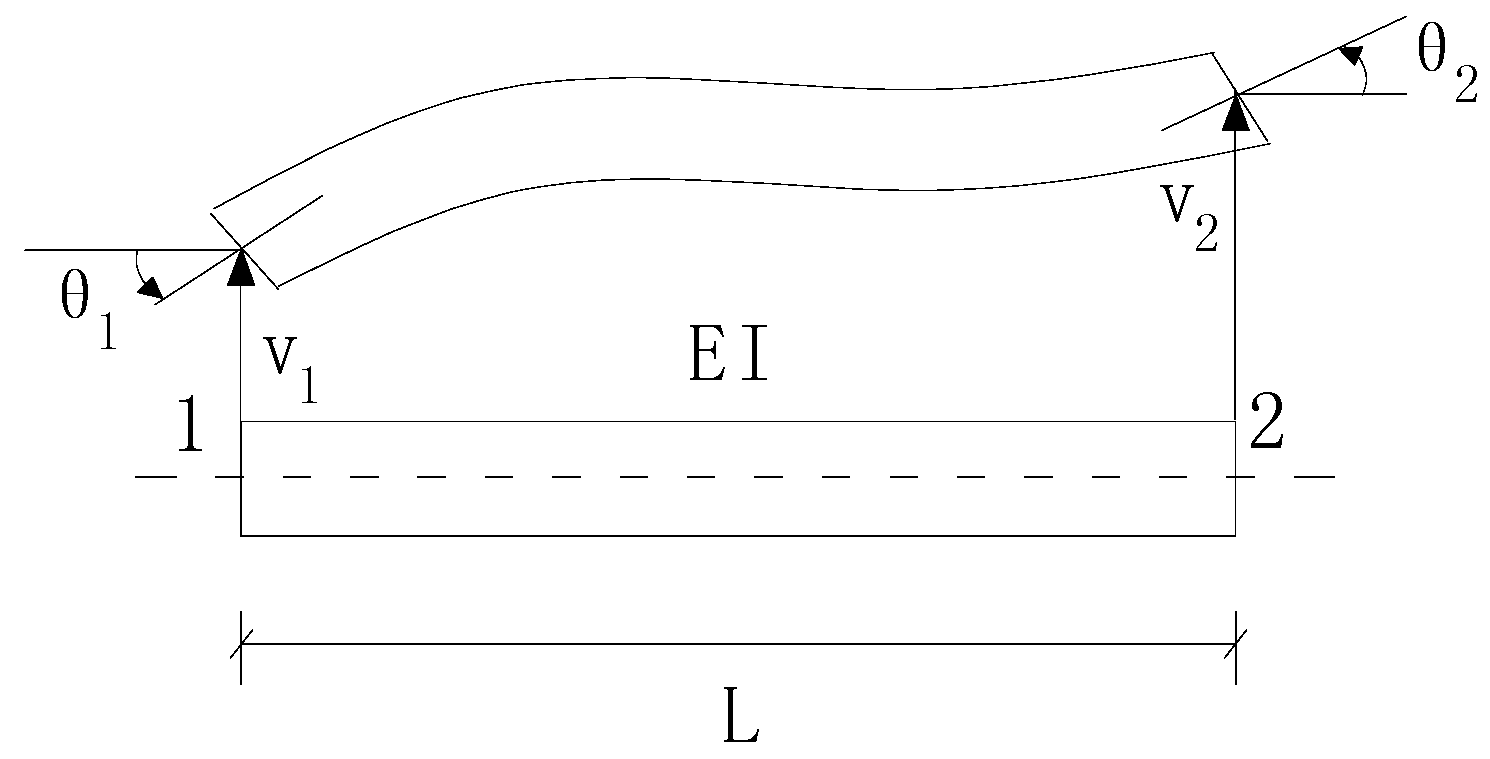
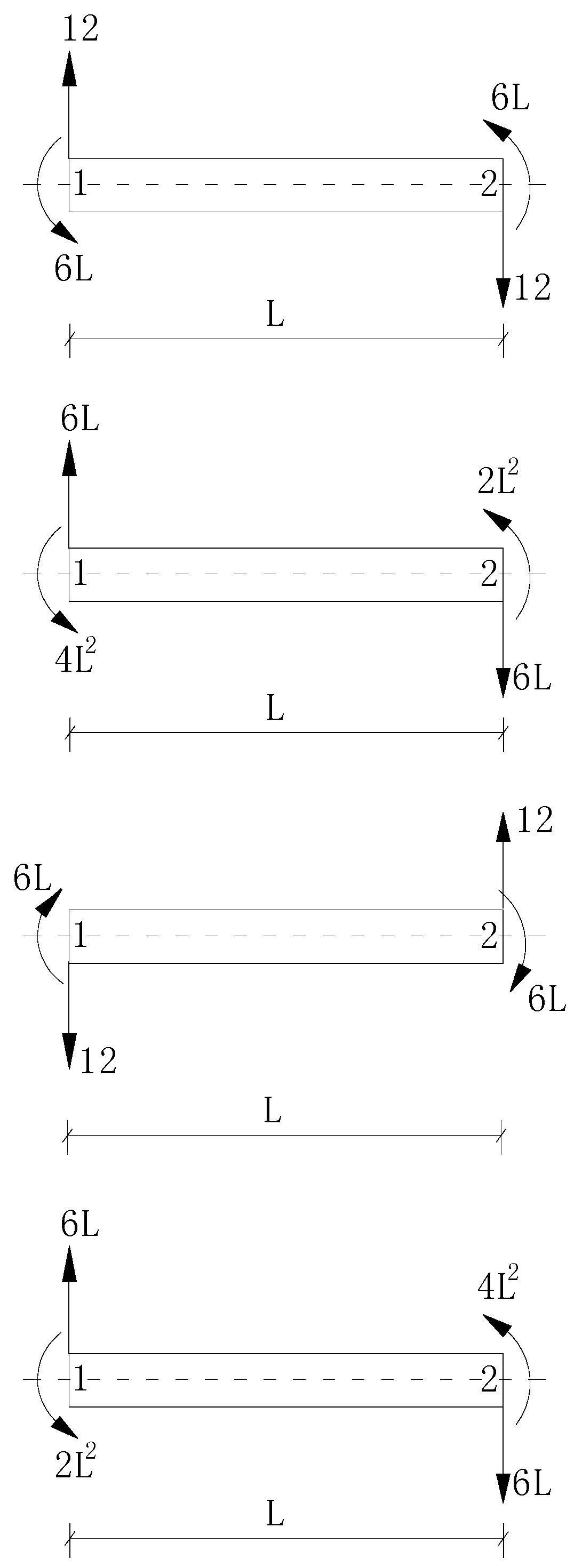
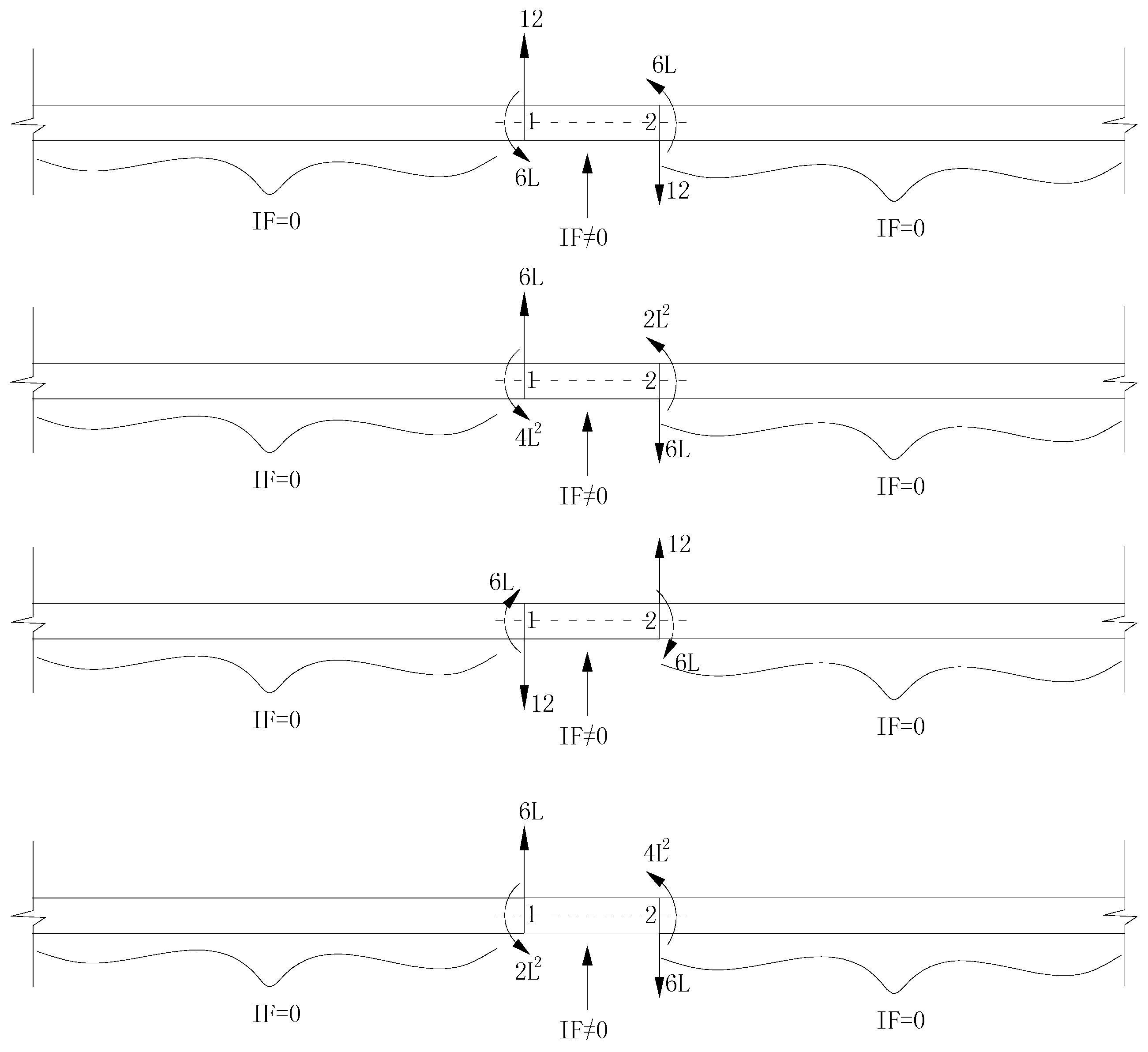
2.1. The Principle of Deflection-Based Damage Localization

In this section, the explicit relation between the defect and defect-induced deformation variation has been derived firstly from the theoretical investigations. Then, the basic principle of deflection-based algorithm for structural damage localization has been illustrated.

For a n-DOFs structure, let K_u and K_d are the stiffness matrices of the intact structure, F_u and F_d are the flexibility matrices of the damaged structures. Then they will satisfy the following relationship:

$$F_u\cdot K_u=F_d\cdot K_d=I_{n\times n}$$

(1)

where I_n×n is the identity matrix. Generally, structural defects reduce the stiffness and increase the flexibility. If ΔK and ΔF are the changes of stiffness and flexibility matrices, then one has:

$$\Delta K=K_u-K_d$$

(2)

$$\Delta F=F_d-F_u$$

(3)

From Equations (1)–(3), one has

$$F_u{K}_u=(F_u+\Delta F)(K_u-\Delta K)$$

(4)

Equation (4) can be expanded as

$$F_u{K}_u=F_u{K}_u-F_u\Delta K+\Delta F(K_u-\Delta K)$$

(5)

From Equation (5), one has

$$F_u\Delta K=\Delta F(K_u-\Delta K)$$

(6)

Substituting Equation (3) into (6) yields

$$F_u\Delta K=\Delta F{K}_d$$

(7)

According to Equation (1), Equation (7) can be rewritten as

$$\Delta F=F_u\Delta K{F}_d$$

(8)

Multiplying Equation (8) by a load vector l, the defect-induced deformation variation vector (DV) can be defined as

$$dv=\Delta Fl=F_u\Delta K{F}_{d}l$$

(9)

According to the FEM theory, the global stiffness change ΔK can be expressed as the summation of all the elemental stiffness changes, i.e.,

$$\Delta K={\displaystyle \sum _{i=1}^{N_e}{\alpha }_i^e}{K}_i^e, (0\le {\alpha }_i^e\le 1)$$

(10)

where ${\alpha }_i^e$ and $K_i^e$ are the damage coefficient and stiffness matrix of the ith element, N_e is the number of elements in the structural FEM. ${\alpha }_i^e=0$ denotes the corresponding element is intact, otherwise the element is damaged. According to Equations (9) and (10), we have

$$dv={\displaystyle \sum _{i=1}^{N_e}(F_u{K}_i^e)({\alpha }_i^e{F}_{d}l)}$$

(11)

According to Equation (11), the DV may be due to a single defect or multiple defects. For brevity, the single defect case is studied firstly in the following discussion. If only ${\alpha }_i^e\ne 0$, Equation (11) can be reduced to

$$dv=(F_u{K}_i^e)({\alpha }_i^e{F}_{d}l)$$

(12)

Let

$$E_i=F_u{K}_i^e$$

(13)

$${\eta }_i={\alpha }_i^e{F}_{d}l$$

(14)

Then Equation (12) simplifies to

$$dv=E_i{\eta }_i$$

(15)

Using the Linear algebra theory [32,33], Equation (15) has important implications that dv is the linear combination of the column vectors in E_i. From Equation (13), E_i is a sparse matrix because the elemental stiffness matrix $K_i^e$ is very sparse. Assuming $e_i^j$ and $k_i^j$ are the jth nonzero column vector of E_i and $K_i^e$, respectively, one has

$$e_i^j=F_u{k}_i^j$$

(16)

According to Equation (16), the physical meaning of the vector $e_i^j$ is the deflection of the intact structure by considering $k_i^j$ as a load vector. Thus, $e_i^j$ is defined as the characteristic deflection and $k_i^j$ is defined as the characteristic force of the ith element. It has been shown from Equation (15) that the deflection variation in a structure due to defect is a linear combination of the characteristic deflections for the damaged element. For the multiple-damage case, a similar conclusion can be obtained using the derivation as before. That is to say, structural deflection variation before and after damage is always the linear combination of the characteristic deflections for those damaged elements.

Now we begin to discuss the properties of the characteristic force and deflection for structural elements. For convenience, the beam element is employed to illustrate these substantive features. Figure 1 presents a Bernoulli-Euler plane beam element with two nodes giving four DOFs, whose stiffness matrix and nodal displacement vector in local co-ordinates are as follows:

$$u^e={[v_1,{\theta }_1,v_2,{\theta }_2]}^T$$

(17)

$$K^e=\frac{EI}{L^3}\left[\begin{array}{cccc}12& 6L& -12& 6L\\ 6L& 4L^2& -6L& 2L^2\\ -12& -6L& 12& -6L\\ 6L& 2L^2& -6L& 4L^2\end{array}\right]$$

(18)

where E is the elastic modulus, I is the moment of inertia, and L is the element length.

The four column vectors of K^e in Equation (18) are the characteristic forces for the Bernoulli-Euler plane beam element in local co-ordinates. Figure 2 shows the corresponding load configurations of these characteristic forces.

From Figure 2, it is apparent that all the load configurations are the self-equilibrating force systems. This conclusion is also valid for other types of finite elements. As can be seen in Figure 3, the internal force (IF) in most parts of the structure under a characteristic force will be zero, except the element associated with this characteristic force.

In short, one can conclude from Figure 2 and Figure 3 that: (1) the characteristic force is a self-equilibrating force; (2) the characteristic force acts only on its own element and not on the rest of the structure. When the characteristic force is applied to the structure without redundant constraints (i.e., the statically determinate structure), only the element associated with the characteristic force is deformed, whereas the remaining part of the structure is not deformed and only has rigid body motion. That is to say, the elemental characteristic deflection will, due to its characteristic force, consist of several parts of the rigid displacement, but not the element itself. As stated before, structural deflection change due to defects is a linear combination of the characteristic deflections corresponding to those damaged elements. Thus, the deflection change of the structure without redundant constraints under an arbitrary load will consist of several parts of the rigid displacement but not the damaged segments. In other words, the turning points between each segment of the rigid displacement in the shape of the deflection change for the structure are the locations of the defects.

For the statically indeterminate structure, the derivation process is the same as that of the statically determinate structure. The only difference is that the IF in some parts of the statically indeterminate structure under a characteristic force will be slightly greater than zero because of the redundant constraint limitation. Correspondingly, the deflection variation due to damage will consist of several parts of the approximate rigid displacement (or the rigid displacement) but not the damaged segments. Then, the turning points between each segment of the approximate rigid displacement (or the rigid displacement) in the deflection change shape are the defect locations. As a result, the sharp peaks in the curvature of structural deflection variation will indicate the locations of structural defects.

2.2. Deflection Estimated by Modal Flexibility Change and PE Method for Damage Localization

In Equation (9), the flexibility change matrix ΔF can be calculated approximately using the first few low-frequency modes, as shown in [34,35]

$$\Delta F={\displaystyle \sum _{j=1}^m\frac{1}{{\lambda }_{dj}}}{\varphi }_{dj}{\varphi }_{dj}^T-{\displaystyle \sum _{j=1}^m\frac{1}{{\lambda }_{uj}}}{\varphi }_{uj}{\varphi }_{uj}^T$$

(19)

where m is the number of measured modes, λ_uj and λ_dj are the eigenvalues of the structure before and after damage, φ_uj and φ_dj are the corresponding eigenvectors, respectively. For the damaged structure, the modal data can be acquired through a modal test in practice. For the intact structure, the modal data are acquired through solving a generalized eigenvalue problem of the undamaged FEM or by the modal experiment.

Using matrix theory [32,33], the principal eigenvector of ΔF can be given by the solutions of the following eigenvalue problem:

$$\Delta F\left(\frac{{\xi }_1}{{\lambda }_1}\right)={\xi }_1$$

(20)

where λ₁ is the principal eigenvalue and ξ₁ is the principal eigenvector of ΔF, respectively. According to Equation (20), the physical meaning of the vector ξ₁ is the structural deflection variation before and after damage by considering $\frac{1}{{\lambda }_1}{\xi }_1$ as a load vector. Thus, according to the principle stated in Section 2.1, structural defects can be located in the following two ways: (1) the turning points in the shape of ξ₁ are the locations of defects; (2) the sharp peaks in the curvature of ξ₁ indicate the locations of structural defects. It is known that the curvature of ξ₁ can be computed using the central difference approximation as follows:

$${({\zeta }_1^i)}^{″}=\frac{{\zeta }_1^{i+1}-2{\zeta }_1^i+{\zeta }_1^{i-1}}{h^2}$$

(21)

where ${\zeta }_1^i$ is the ith coefficient of ξ₁, h is the length of structural element, and ${({\zeta }_1^i)}^{″}$ is the ith curvature coefficient of ξ₁.

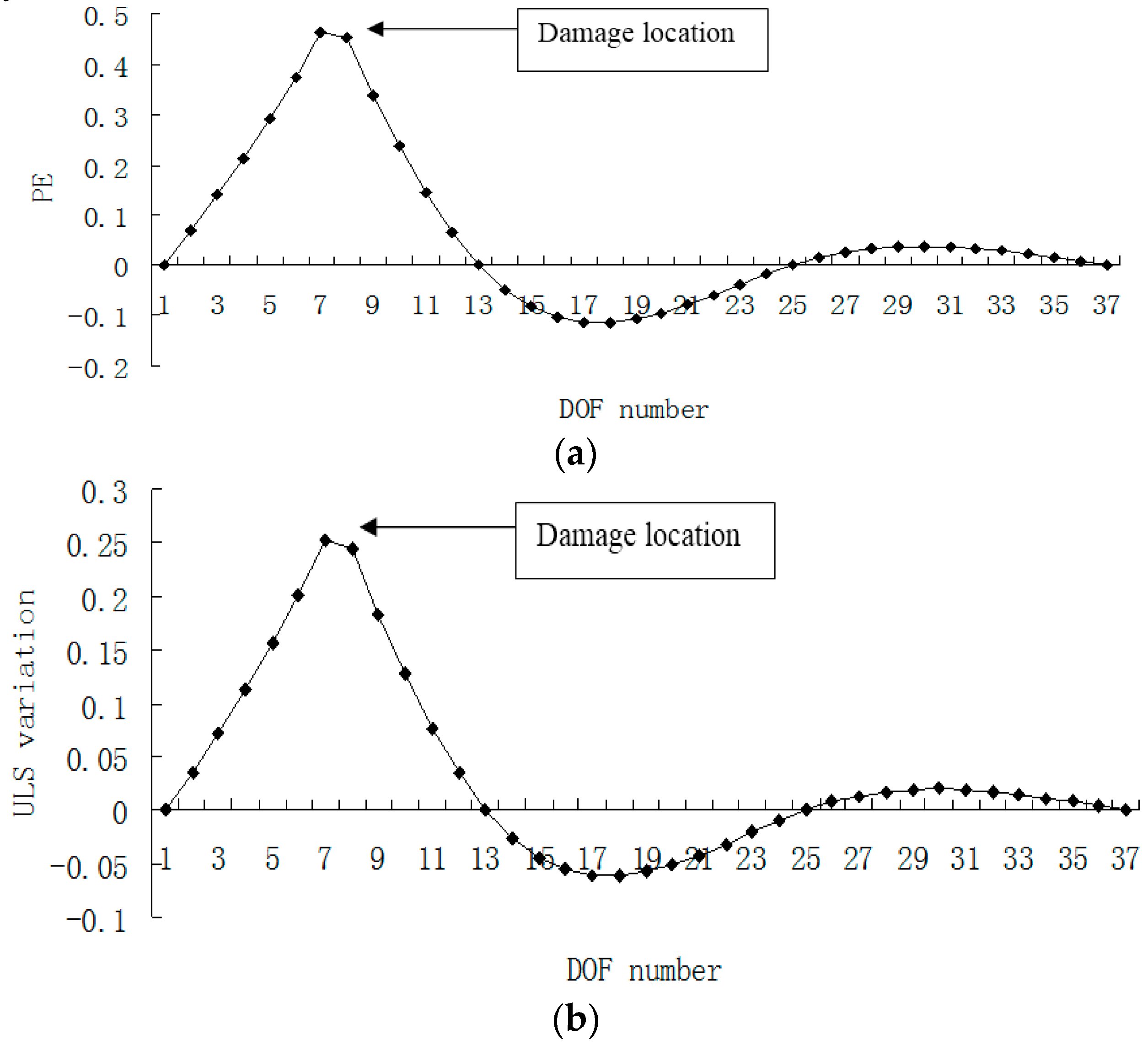
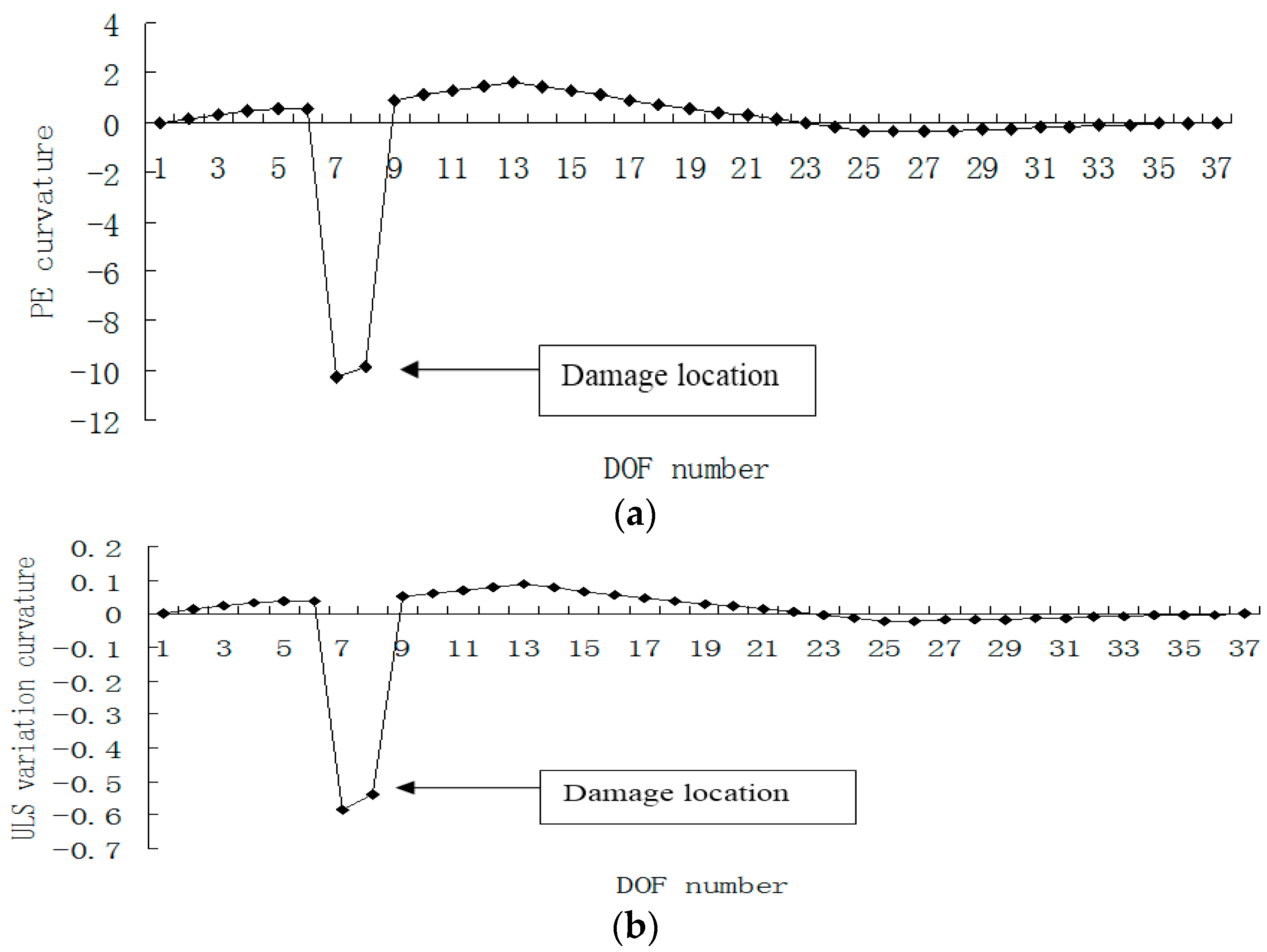
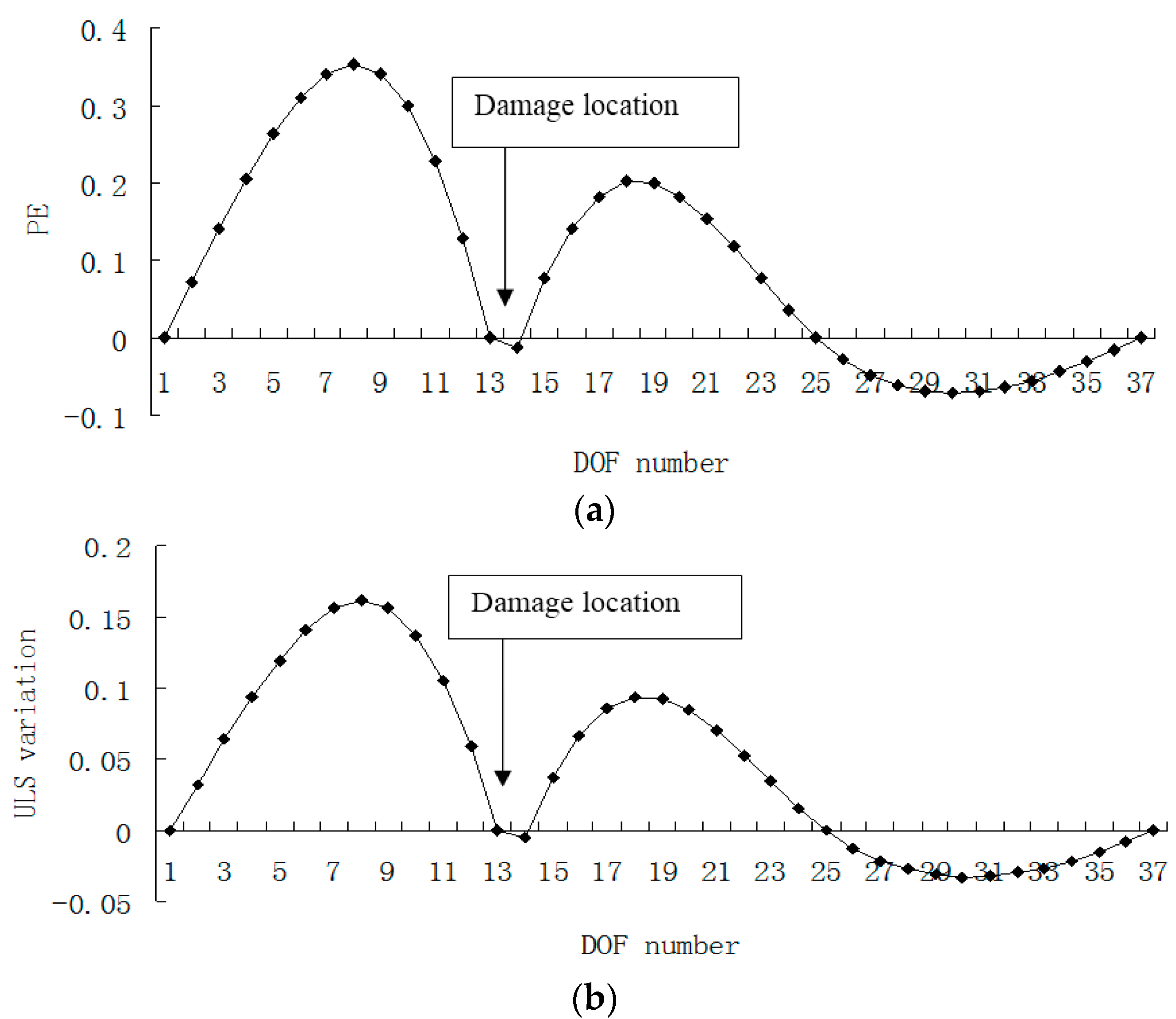
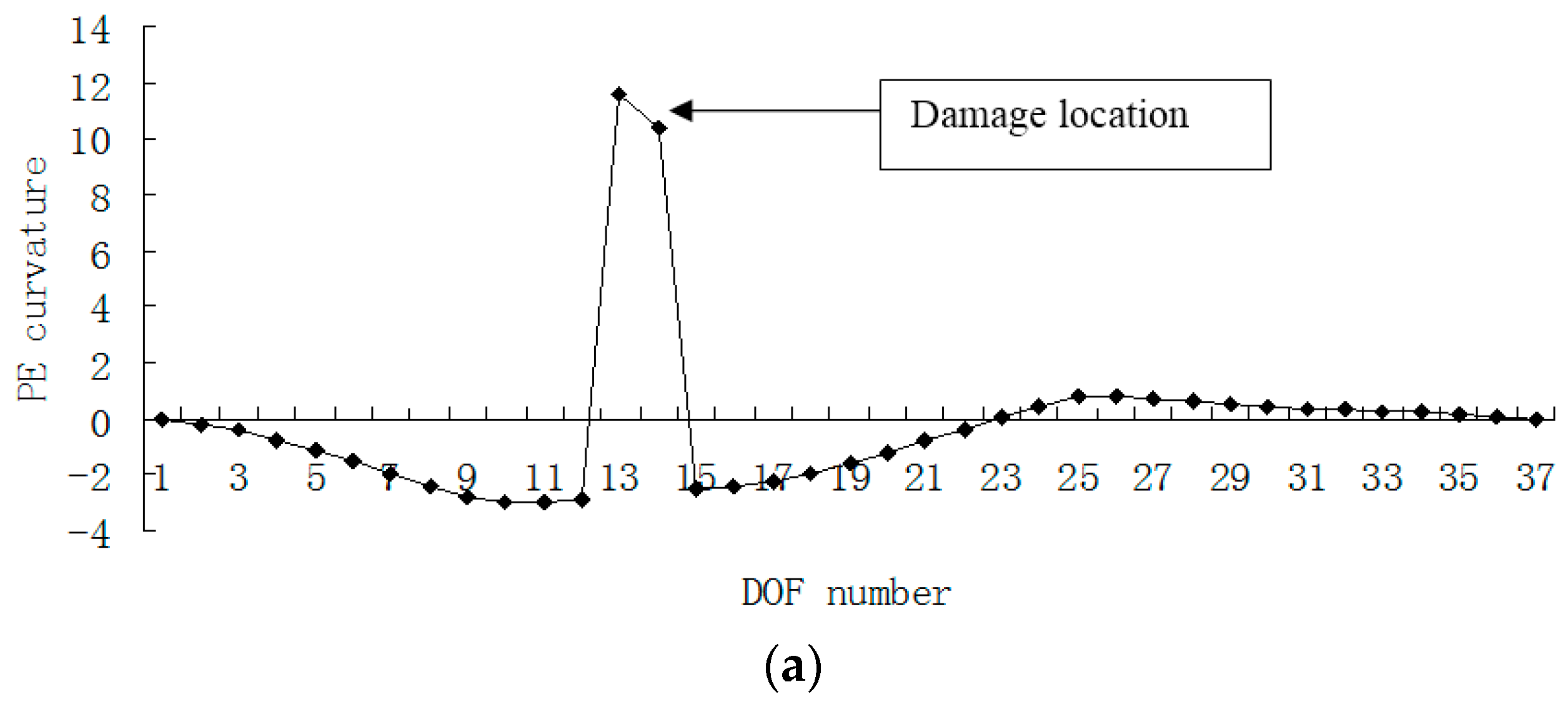
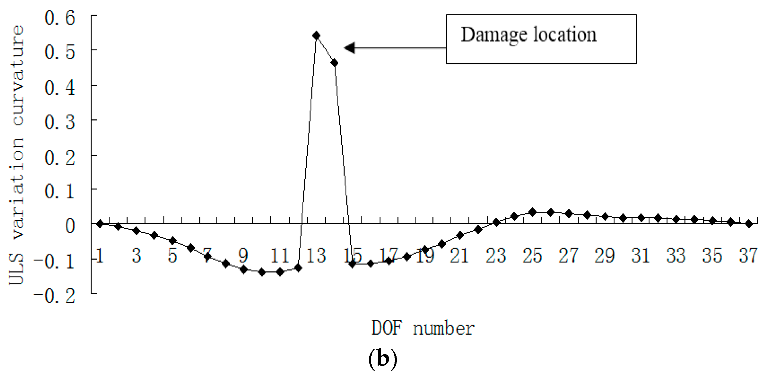
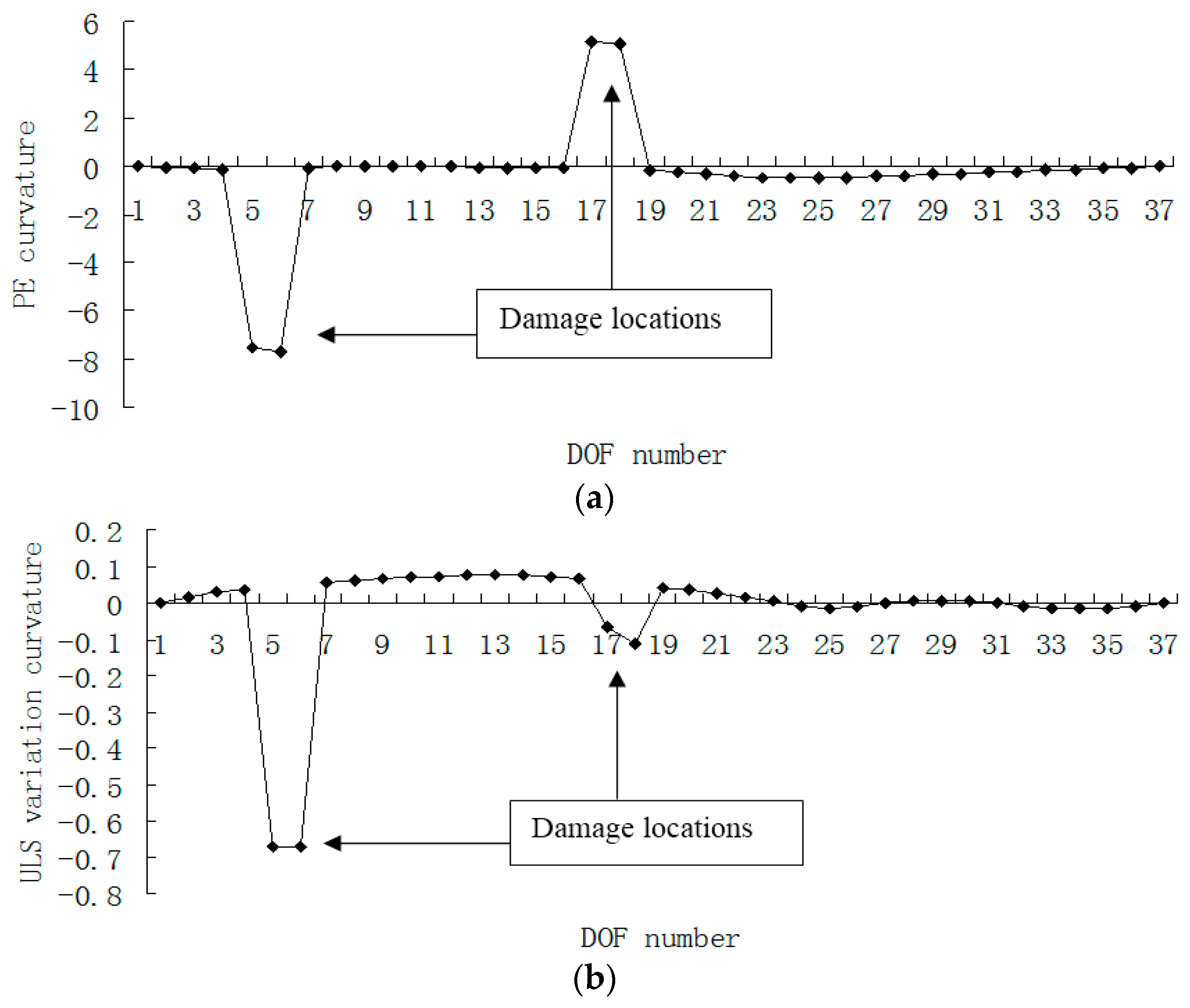
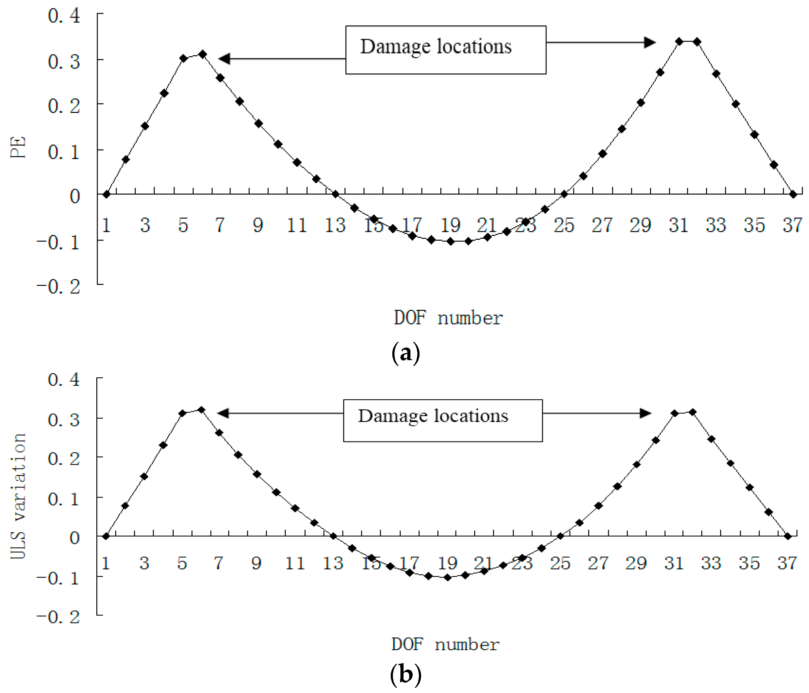
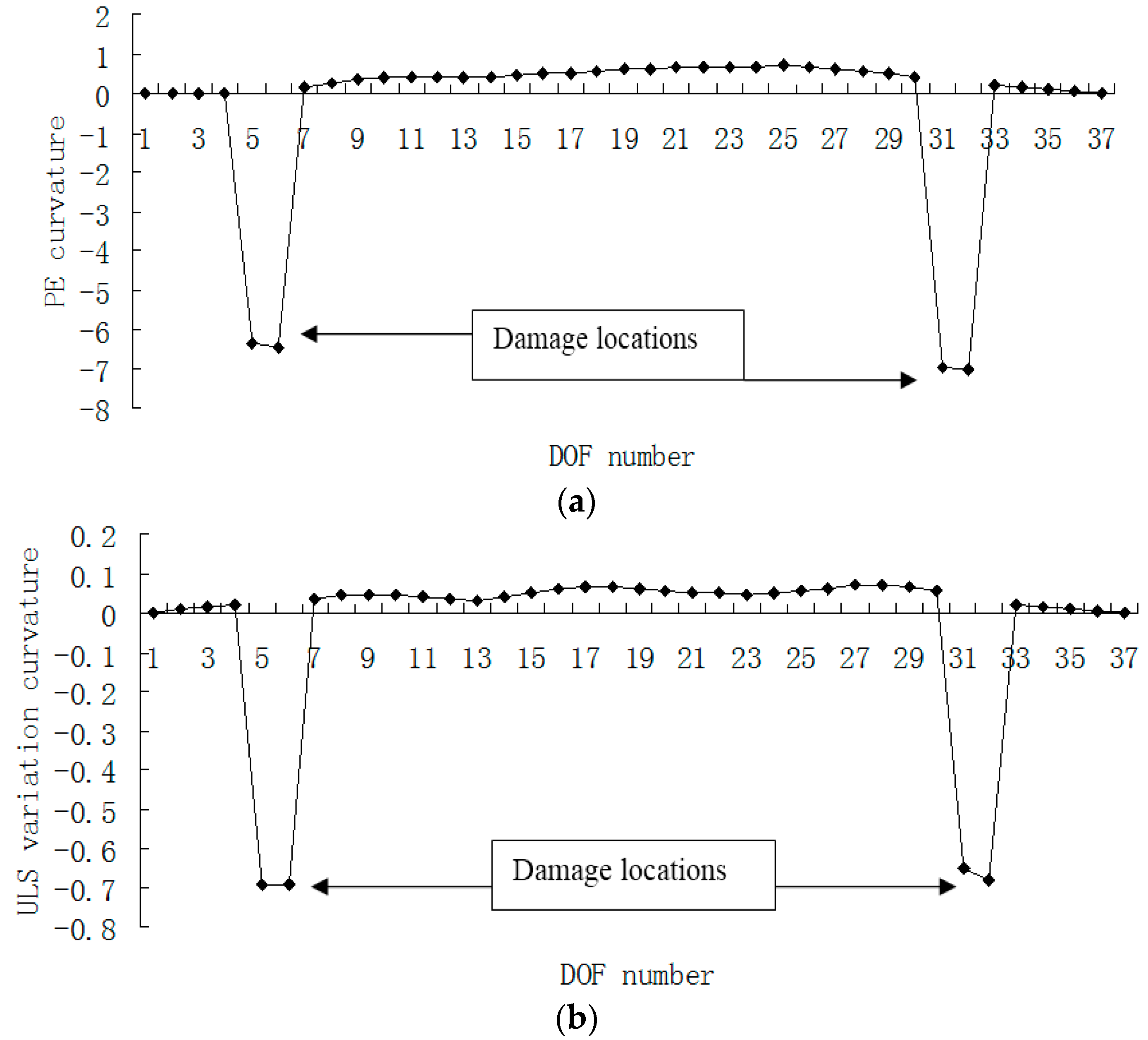
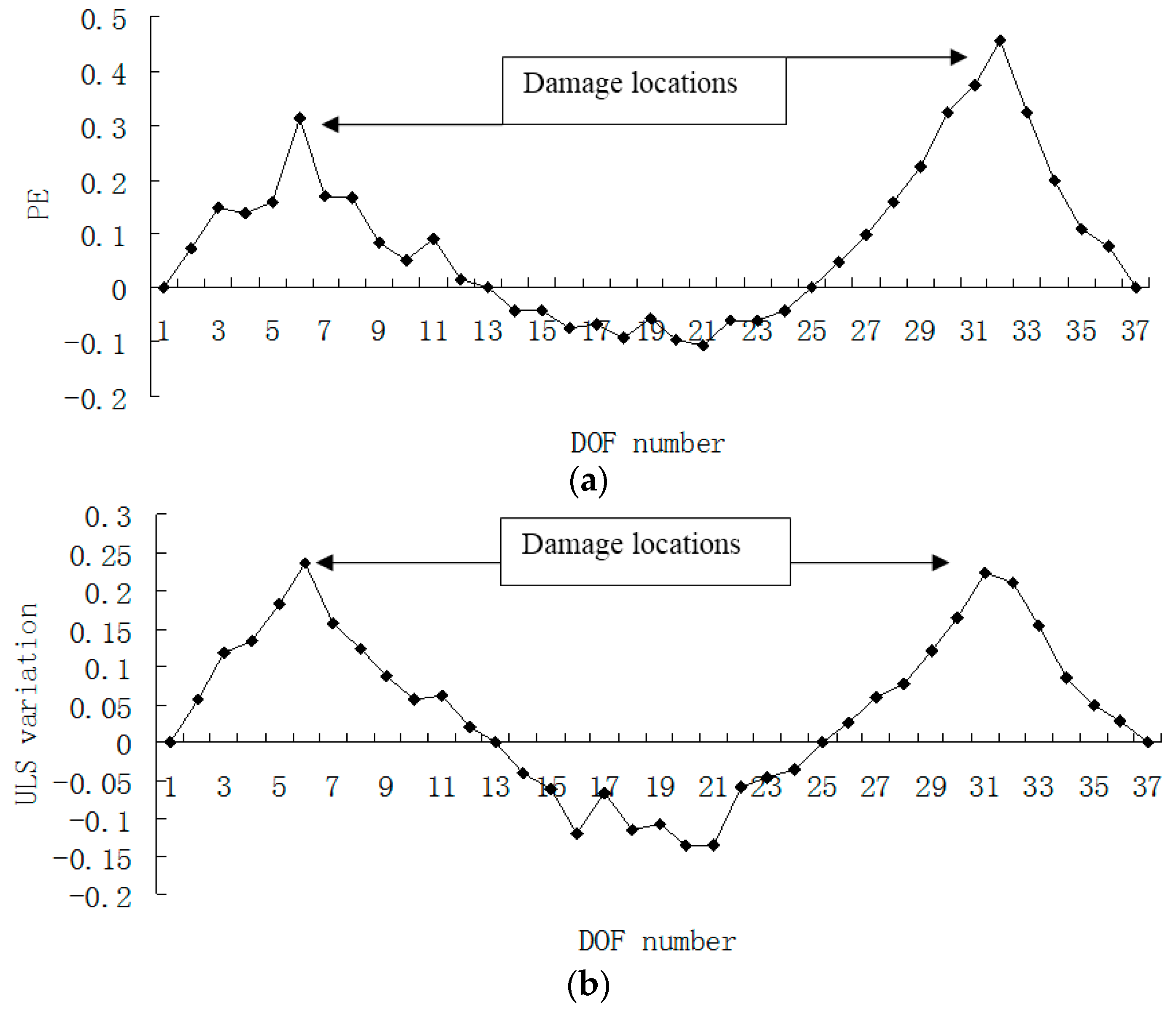
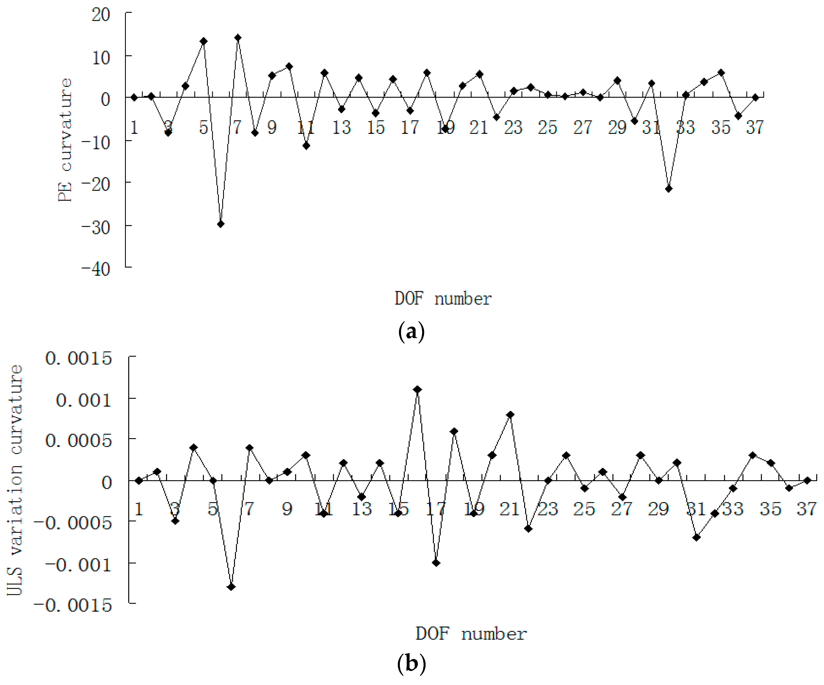
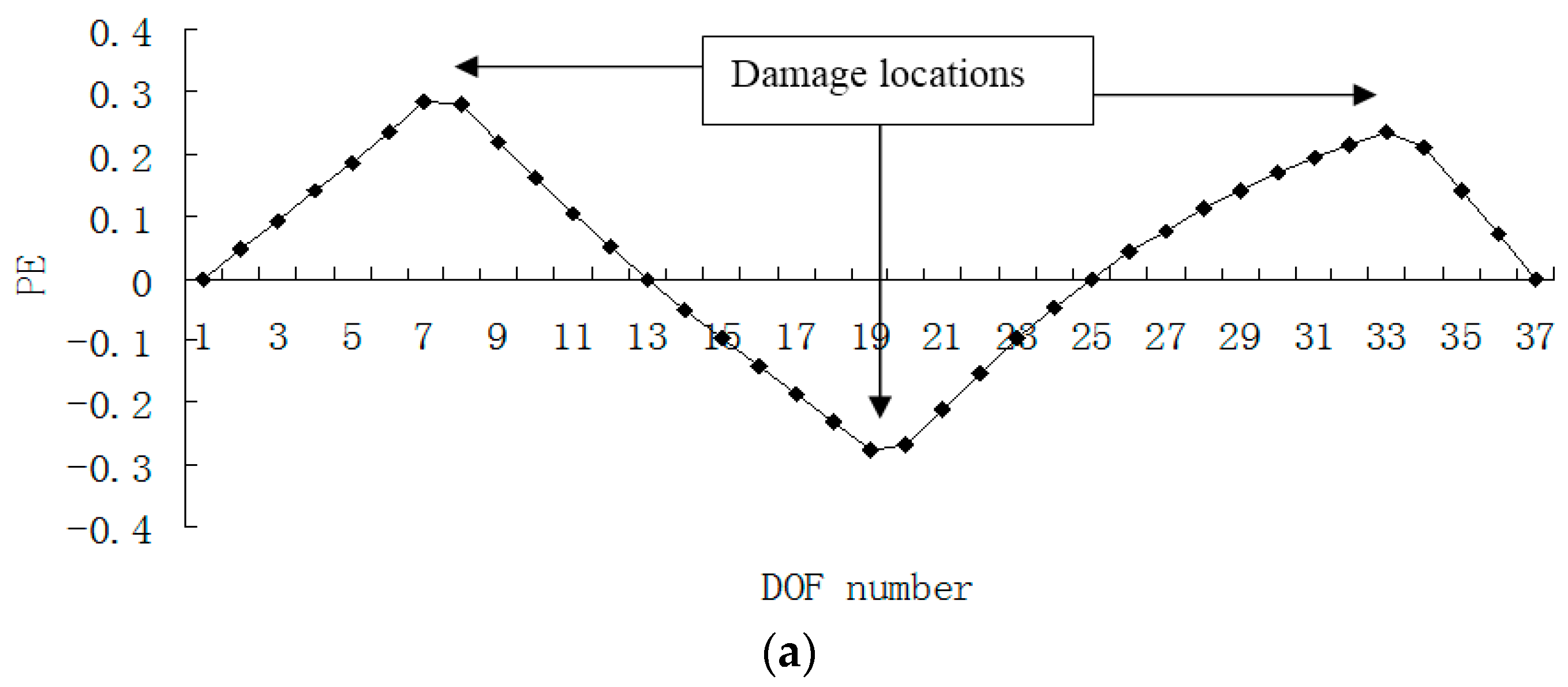
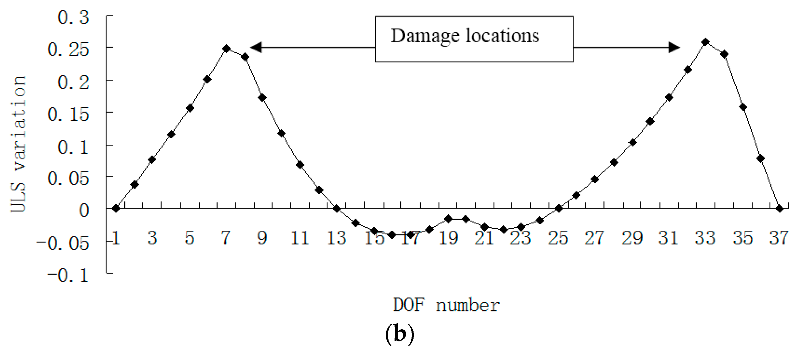
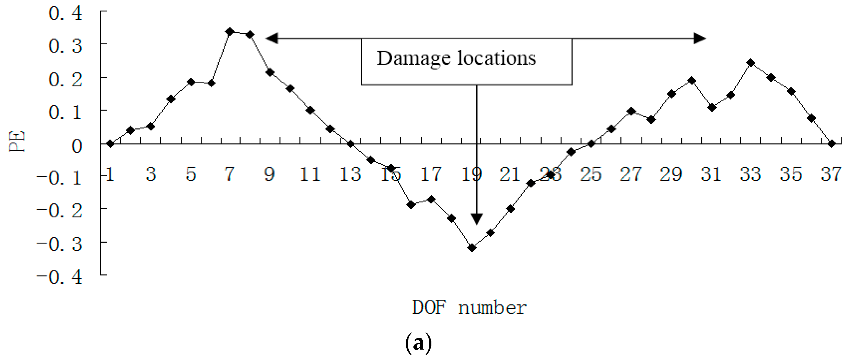
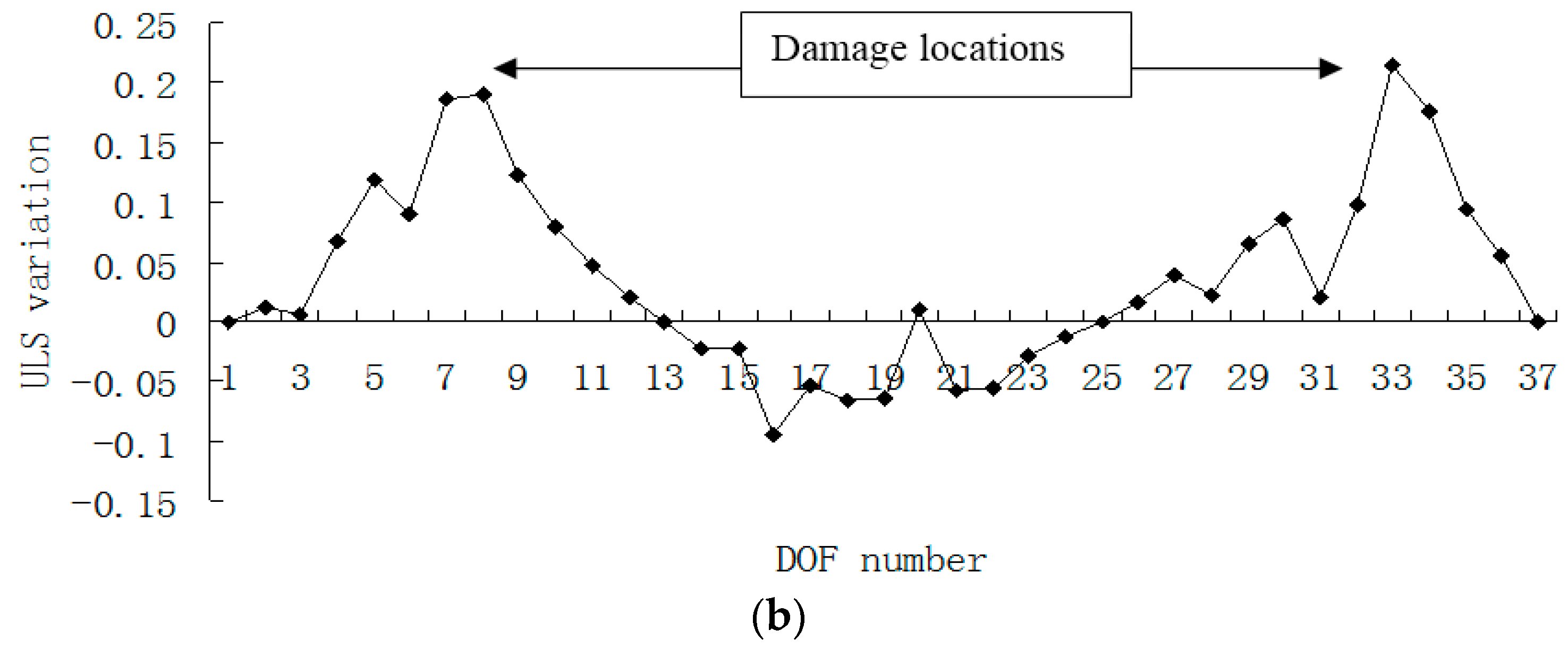
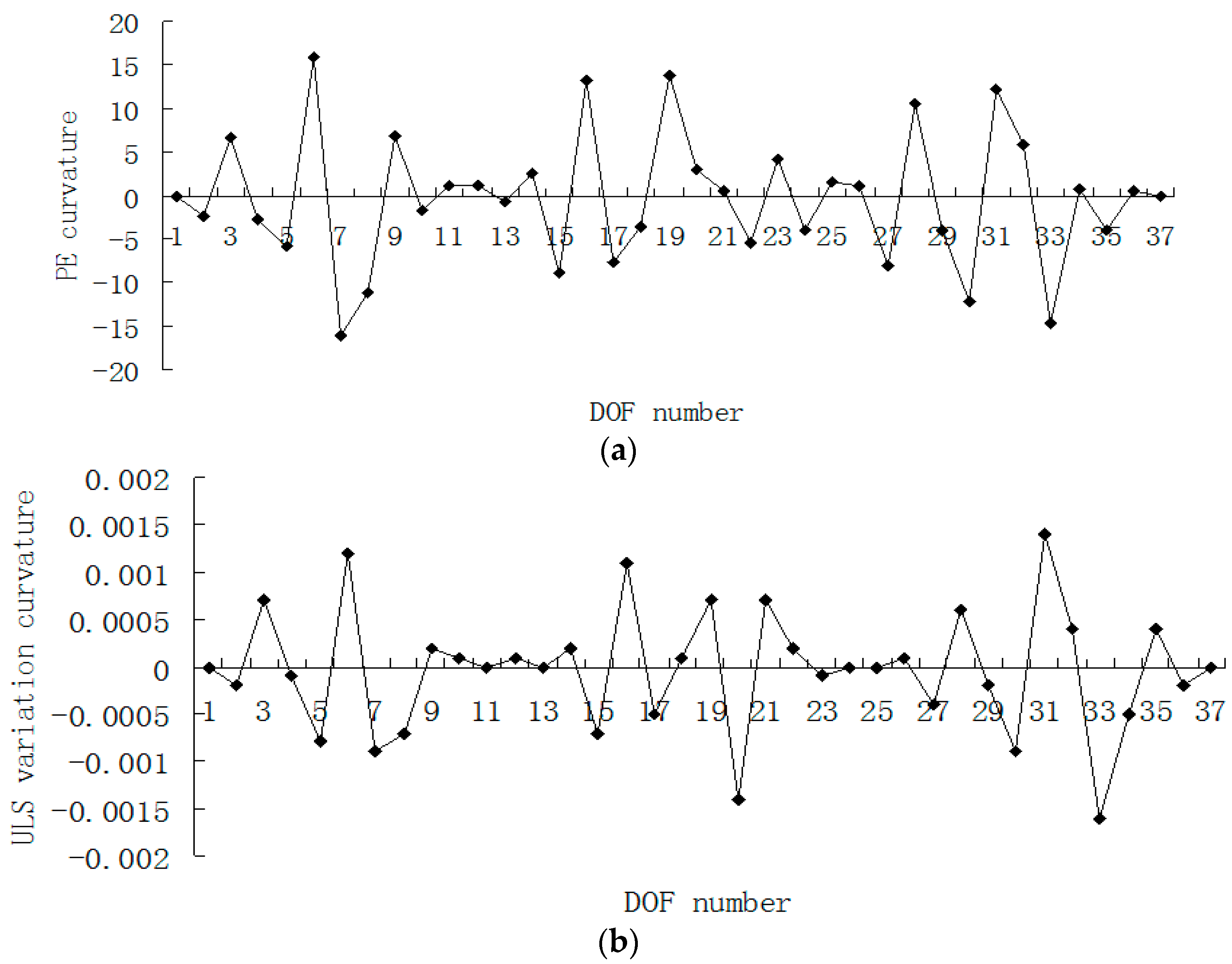
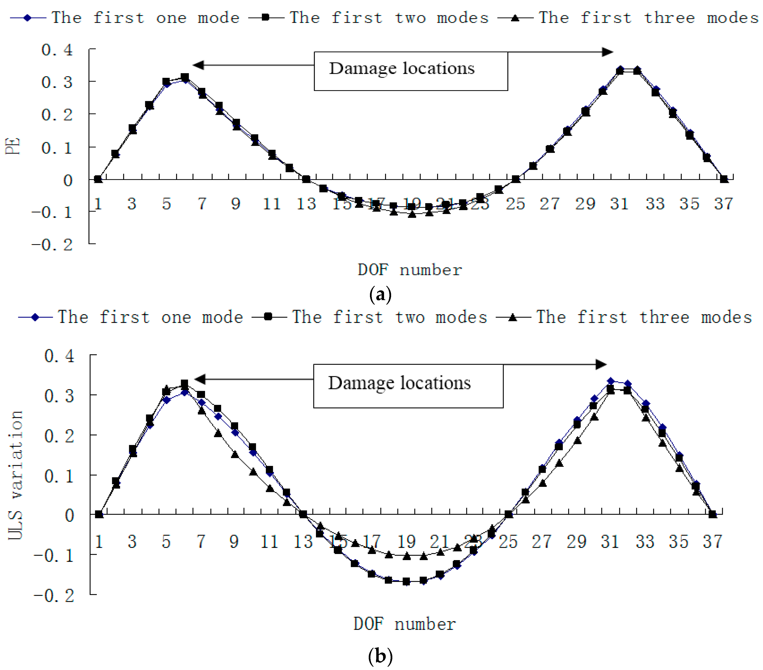
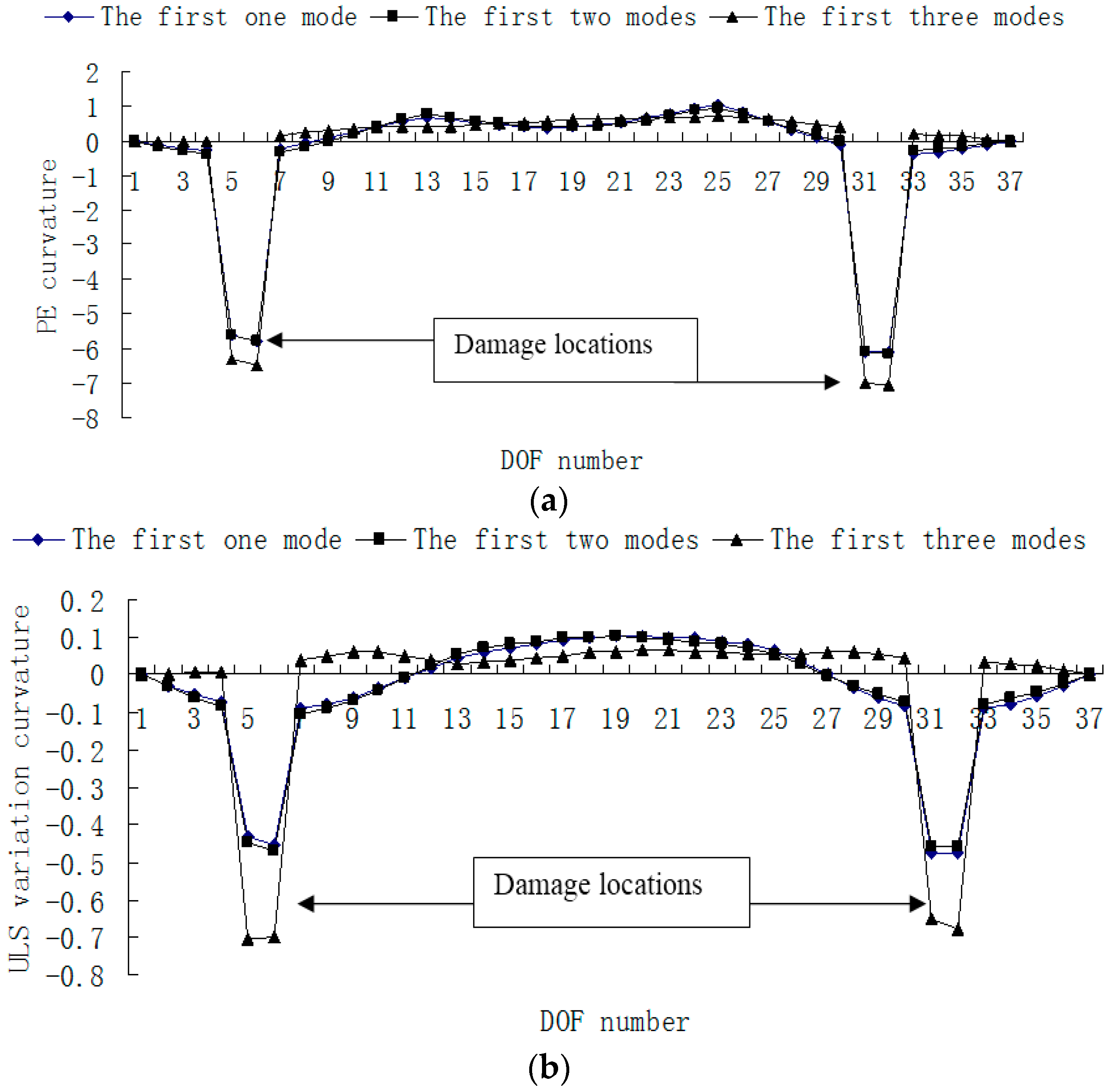
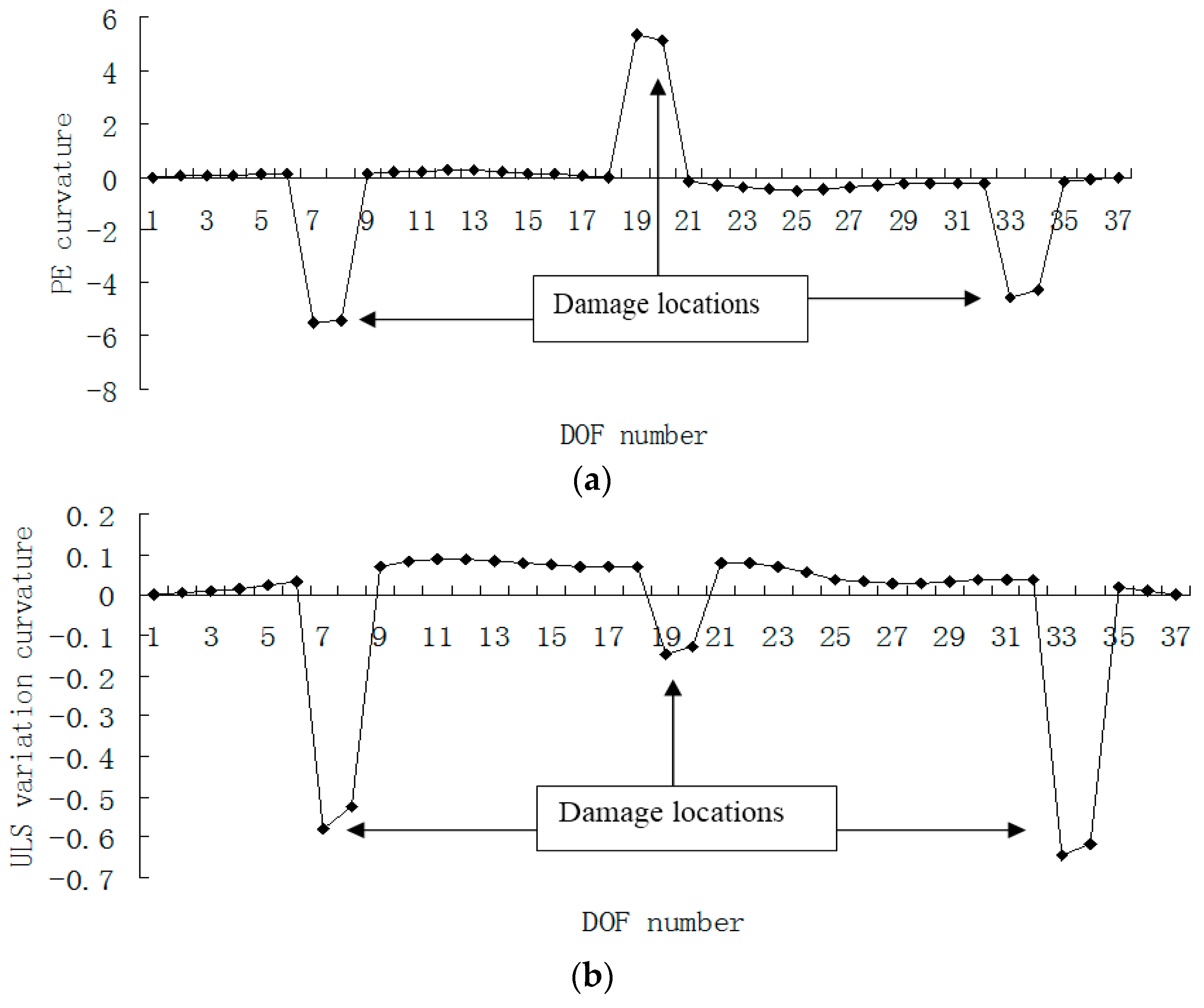
3. Numerical Example

The continuous beam in Figure 4 is used to demonstrate the defect localization ability of the presented PE algorithm.

Note that this example is a statically indeterminate structure. For the structure, the elastic modulus, density, moment of inertia, and cross-sectional area are 200 GPa, 7.8 × 10³ Kg/m³, 1.0416 × 10⁻⁶ m⁴, 0.0025 m², respectively. In the FEM, the structure is divided into 36 elements, which gives 33 translational DOFs and 37 rotational DOFs. The length of each segment in the beam FEM is 0.1 m. In the following discussion, only the first four modal parameters with the translational degrees of freedom are used in order to simulate the incomplete measurements. Defect in the beam was simulated by reducing the elastic modulus of some structural elements. Five defect scenarios are assumed in the example. Scenario 1: the defect occurred in element 7 with 20% stiffness reduction. Scenario 2: the defect occurred in element 13 with 20% stiffness reduction. Scenario 3: the defects occurred in elements 5 and 17 both with 20% stiffness reduction. Scenario 4: the defects occurred in elements 5 and 31 both with 20% stiffness reduction. Scenario 5: the defects occurred in elements 7, 19 and 33 all with 20% stiffness reduction. Detection results of each damage scenario obtained by the presented PE algorithm and the well-known ULS method are both given to compare the localization performance.

Using the exact data without noise, the principal eigenvector (PE) of modal flexibility change and the ULS variation for damage scenario 1 are plotted in Figure 5a,b, respectively. Accordingly, the PE curvature and the ULS variation curvature for the case of damage scenario 1 are plotted in Figure 6a,b, respectively.

One can see that the transnational DOFs numbered 7 and 8 are the turning points in Figure 5 and the sharp peaks in Figure 6, respectively. In the beam model, the seventh and the eighth transnational DOFs are exactly corresponding to the seventh element. This means that the seventh segment could be successfully detected to be the defect area by inspecting the turning points in Figure 5, or by inspecting the sharp peaks in Figure 6. Note that the human inspection and intervention is required in the above damage localization process.

Damage scenario 2 is used to verify the validity of the two algorithms when the defect occurred near the supported boundary. Figure 7 and Figure 8 showed the detection results of this scenario. One can conclude that the damaged element 13 can be detected by inspecting the turning points in Figure 7, or by inspecting the sharp peaks in Figure 8.

Damage cases 3–5 are used to compare the PE algorithm with the ULS method for the multiple damage scenarios. Figure 9 and Figure 10 showed the results of damage localization for damage case 3. From Figure 9a and Figure 10a, one can see that the damaged elements 5 and 17 were clearly identified by PE and PE curvature. From Figure 9b, the ULS variation method fails to detect the damaged element 17. It can be seen from Figure 10 that the PE curvature provides comparatively better damage location predictions than the ULS curvature.

Figure 11, Figure 12, Figure 13 and Figure 14 presented the damage localization results for damage case 4 using the exact modal data and the data with 3% noise, respectively. From Figure 11 and Figure 12, both damage localization methods can achieve satisfactory results by using error-free data.

From Figure 13, one can see that the indexes of PE and ULS variation can still identify the damaged elements 5 and 31 even if 3% noise is considered. According to Figure 14, it is apparent that the curvature indexes are seriously affected by the measurement error, and the damaged segments cannot be determined by these curvature maps with noise.

Figure 15, Figure 16, Figure 17 and Figure 18 presented the damage localization results for damage case 5 using the exact modal data and the data with 3% noise, respectively. From Figure 15a and Figure 16a, one can see that the damaged elements 7, 19 and 33 were clearly identified by PE and PE curvature. From Figure 15b, the ULS variation method fails to detect the damaged element 19. It can be concluded that the PE algorithm can precisely identify multiple defect locations, whereas the ULS method occasionally missed multiple damage locations.

From Figure 17, one can see that the indexes of PE and ULS variation can still identify the damaged elements 7, 19 and 33 even if 3% noise is considered. From Figure 18, it is apparent that the curvature indexes are seriously affected by the measurement error, and the damaged locations cannot be determined by these curvature maps with noise.

In order to study the sensitivity of the proposed method to the number of modes, Figure 19 and Figure 20 give the damage localization results of damage case 4 using the first one, two and three modes without noise, respectively. From Figure 19 and Figure 20, one can see that the ULS method is more sensitive to the number of modes than the PE method, and both damage localization methods can achieve reasonable results, even if only the first mode without noise is used in the calculation.

4. Conclusions

A new vibration-based method has been developed for structural damage localization, which is based on the principal eigenvector (PE) of modal flexibility change. In order to verify the feasibility of the PE algorithm, a three-span continuous beam was investigated for several damage scenarios with and without noise. Furthermore, the PE method was compared with the well-known ULS method to show its advantages. According to the numerical results, the presented PE method may be more effective at identifying the defect locations of the beam structure than the ULS method. The proposed PE procedure may have good prospects in structural damage localization.

References

1. Doebling, S.W.; Farrar, C.R.; Prime, M.B. A summary review of vibration-based damage identification methods. Shock Vib. Dig. 1998, 30, 91–105. [Google Scholar] [CrossRef]
2. Carden, E.P.; Fanning, P. Vibration based condition monitoring: A review. Struct. Health Monit. 2004, 3, 355–377. [Google Scholar] [CrossRef]
3. Prinaris, A.; Alampalli, S.; Ettouney, M. Review of remote sensing for condition assessment and damage identification after extreme loading conditions. In Proceedings of the 2008 Structures Congress, Vancouver, BC, Canada, 24–26 April 2008.
4. Ashokkumar, C.R.; Lyengar, N.G.R. Partial eigenvalue assignment for structural damage mitigation. J. Sound Vib. 2011, 330, 9–16. [Google Scholar] [CrossRef]
5. Yang, Z.C.; Wang, L. Structural damage detection by changes in natural frequencies. J. Intell. Mater. Syst. Struct. 2010, 21, 309–319. [Google Scholar] [CrossRef]
6. Zhu, H.P.; Li, L.; He, X.Q. Damage detection method for shear buildings using the changes in the first mode shape slopes. Comput. Struct. 2011, 89, 733–743. [Google Scholar] [CrossRef]
7. Weber, B.; Paultre, P. Damage identification in a truss tower by regularized model updating. J. Struct. Eng. 2010, 136, 1943–1953. [Google Scholar] [CrossRef]
8. Adewuyi, A.P.; Wu, Z.S. Modal macro-strain flexibility methods for damage localization in flexural structures using long-gage FBG sensors. Struct. Control Health Monit. 2011, 18, 341–360. [Google Scholar] [CrossRef]
9. Limongelli, M.P. Frequency response function interpolation for damage detection under changing environment. Mech. Syst. Signal Process. 2010, 24, 2898–2913. [Google Scholar] [CrossRef]
10. Lima, A.M.G.; Faria, A.W.; Rade, D.A. Sensitivity analysis of frequency response functions of composite sandwich plates containing viscoelastic layers. Compos. Struct. 2010, 92, 364–376. [Google Scholar] [CrossRef]
11. Lu, Z.R.; Law, S.S. Differentiating different types of damage with response sensitivity in time domain. Mech. Syst. Signal Process. 2010, 24, 2914–2928. [Google Scholar] [CrossRef]
12. Lu, Z.R.; Huang, M.; Liu, J.K. State-space formulation for simultaneous identification of both damage and input force from response sensitivity. Smart Struct. Syst. 2011, 8, 157–172. [Google Scholar] [CrossRef]
13. Wong, C.N.; Huang, H.Z.; Xiong, J.Q.; Lan, H.L. Generalized-order perturbation with explicit coefficient for damage detection of modular beam. Arch. Appl. Mech. 2011, 81, 451–472. [Google Scholar] [CrossRef]
14. Yang, Q.W. A new damage identification method based on structural flexibility disassembly. J. Vib. Control 2011, 17, 1000–1008. [Google Scholar] [CrossRef]
15. Yang, Q.W.; Sun, B.X. Structural damage localization and quantification using static test data. Struct. Health Monit. 2011, 10, 381–389. [Google Scholar] [CrossRef]
16. Yang, Q.W.; Liu, J.K.; Li, C.H.; Liang, C.F. A Universal fast algorithm for sensitivity-based structural damage detection. Sci. World J. 2013, 2013. [Google Scholar] [CrossRef] [PubMed]
17. Zhang, Z.; Aktan, A.E. Application of modal flexibility and its derivatives in structural identification. Res. Nondestruct. Eval. 1998, 10, 43–61. [Google Scholar] [CrossRef]
18. Wu, D.; Law, S.S. Damage localization in plate structures from uniform load surface curvature. J. Sound Vib. 2004, 276, 227–244. [Google Scholar] [CrossRef]
19. Wu, D.; Law, S.S. Sensitivity of uniform load surface curvature for damage identification in plate structures. J. Vib. Acoust. 2005, 127, 84–92. [Google Scholar] [CrossRef]
20. Wang, J.; Qiao, P.Z. Improved damage detection for beam-type structures using a uniform load surface. Struct. Health Monit. 2007, 6, 99–110. [Google Scholar] [CrossRef]
21. Choi, I.Y.; Lee, J.S.; Choi, E.; Cho, H.N. Development of elastic damage load theorem for damage detection in a statically determinate beam. Comput. Struct. 2004, 82, 2483–2492. [Google Scholar] [CrossRef]
22. Sung, S.H.; Jung, H.J.; Jung, H.Y. Damage detection of beam-like structures using the normalized curvature of a uniform load surface. J. Sound Vib. 2013, 332, 1501–1519. [Google Scholar] [CrossRef]
23. Tomaszewska, A. Influence of statistical errors on damage detection based on structural flexibility and mode shape curvature. Comput. Struct. 2010, 88, 154–164. [Google Scholar] [CrossRef]
24. Koo, K.Y.; Lee, J.J.; Yun, C.B.; Kim, J.T. Damage detection in beam-like structures using deflections obtained by modal flexibility matrices. Smart Struct. Syst. 2008, 4, 605–628. [Google Scholar] [CrossRef]
25. Qiao, P.; Lu, K.; Lestari, W.; Wang, J. Curvature mode shape-based damage detection in composite laminated plates. Compos. Struct. 2007, 80, 409–428. [Google Scholar] [CrossRef]
26. Fan, W.; Qiao, P. Vibration-based damage identification methods: A review and comparative study. Struct. Health Monit. 2011, 10, 83–111. [Google Scholar] [CrossRef]
27. Hamze, A.; Gueguen, P.; Roux, P.; Baillet, L. Comparative study of damage identification algorithms applied to a Plexiglas beam. In Proceedings of the 15th International Conference on Experimental Mechanics, Porto, Portuga, 22–27 July 2012; pp. 22–27.
28. Domaneschi, M.; Limongelli, M.P.; Martinelli, L. Vibration based damage localization using MEMS on a suspension bridge model. Smart Struct. Syst. 2013, 12, 679–694. [Google Scholar] [CrossRef]
29. Domaneschi, M.; Limongelli, M.P.; Martinelli, L. Damage detection and localization on a benchmark cable-stayed bridge. Earthq. Struct. 2015, 8, 1113–1126. [Google Scholar] [CrossRef]
30. Manoach, E.; Samborski, S.; Mitura, A.; Warminski, J. Vibration based damage detection in composite beams under temperature variations using Poincare maps. Int. J. Mech. Sci. 2012, 62, 120–132. [Google Scholar] [CrossRef]
31. Manoach, E.; Trendafilova, I. Large amplitude vibrations and damage detection of rectangular plates. J. Sound Vib. 2008, 315, 591–606. [Google Scholar] [CrossRef] [Green Version]
32. Herstein, I.N.; Winter, D.J. Matrix Theory and Linear Algebra; Macmillan Publishing Company: Indianapolis, IN, USA, 1988. [Google Scholar]
33. Datta, B.N. Numerical Linear Algebra and Applications; Brooks/Cole Publishing Company: Pacific Grove, CA, USA, 1995. [Google Scholar]
34. Pandey, A.K.; Biswas, M. Damage detection in structures using changes in flexibility. J. Sound Vib. 1994, 169, 3–17. [Google Scholar] [CrossRef]
35. Pandey, K.; Biswas, M. Experimental verification of flexibility difference method for locating damage in structures. J. Sound Vib. 1995, 184, 311–328. [Google Scholar] [CrossRef]
Figure 1. A Bernoulli-Euler plane beam element
Algorithms 09 00024 g001
Figure 2. Load configurations of the four characteristic forces.
Algorithms 09 00024 g002
Figure 3. The internal force (IF) distributions of the structure under characteristic forces.
Algorithms 09 00024 g003
Figure 4. A beam structure with three spans.
Algorithms 09 00024 g004
Figure 5. (a) Damage index (principal eigenvector (PE)) map using the first four exact modes when the defect occurred in element 7; (b) Damage index (uniform load surface (ULS) variation) map using the first four exact modes when the defect occurred in element 7 (×10−4).
Algorithms 09 00024 g005
Figure 6. (a) Damage index (PE curvature) map using the first four exact modes when the defect occurred in element 7; (b) Damage index (ULS variation curvature) map using the first four exact modes when the defect occurred in element 7 (×10−3).
Algorithms 09 00024 g006
Figure 7. (a) Damage index (PE) map using the first four exact modes when the defect occurred in element 13; (b) Damage index (ULS variation) map using the first four exact modes when the defect occurred in element 13(×10−4).
Algorithms 09 00024 g007
Figure 8. (a) Damage index (PE curvature) map using the first four exact modes when the defect occurred in element 13; (b) Damage index (ULS variation curvature) map using the first four exact modes when the defect occurred in element 13 (×10−3).
Algorithms 09 00024 g008aAlgorithms 09 00024 g008b
Figure 9. (a) Damage index (PE) map using the first four exact modes when the defects occurred in elements 5 and 17; (b) Damage index (ULS variation) map using the first four exact modes when the defects occurred in elements 5 and 17 (×10−4).
Algorithms 09 00024 g009
Figure 10. (a) Damage index (PE curvature) map using the first four exact modes when the defects occurred in elements 5 and 17; (b) Damage index (ULS variation curvature) map using the first four exact modes when the defects occurred in elements 5 and 17 (×10−3).
Algorithms 09 00024 g010
Figure 11. (a) Damage index (PE) map using the first four exact modes when the defects occurred in elements 5 and 31; (b) Damage index (ULS variation) map using the first four exact modes when the defects occurred in elements 5 and 31 (×10−4).
Algorithms 09 00024 g011
Figure 12. (a) Damage index (PE curvature) map using the first four exact modes when the defects occurred in elements 5 and 31; (b) Damage index (ULS variation curvature) map using the first four exact modes when the defects occurred in elements 5 and 31 (×10−3).
Algorithms 09 00024 g012
Figure 13. (a) Damage index (PE) map using the first four modes with 3% noise when elements 5 and 31 are damaged; (b) Damage index (ULS variation) map using the first four modes with 3% noise when elements 5 and 31 are damaged (×10−4).
Algorithms 09 00024 g013
Figure 14. (a) Damage index (PE curvature) map using the first four modes with 3% noise when elements 5 and 31 are damaged; (b) Damage index (ULS variation curvature) map using the first four modes with 3% noise when elements 5 and 31 are damaged (×10−3).
Algorithms 09 00024 g014
Figure 15. (a) Damage index (PE) map using the first four exact modes when the defects occurred in elements 7, 19 and 33; (b) Damage index (ULS variation) map using the first four exact modes when the defects occurred in elements 7, 19 and 33 (×10−4).
Algorithms 09 00024 g015aAlgorithms 09 00024 g015b
Figure 16. (a) Damage index (PE curvature) map using the first four modes without noise when elements 7, 19 and 33 are damaged; (b) Damage index (ULS variation curvature) map using the first four modes without noise when elements 7, 19 and 33 are damaged (×10−3).
Algorithms 09 00024 g016
Figure 17. (a) Damage index (PE) map using the first four modes with 3% noise when elements 7, 19 and 33 are damaged; (b) Damage index (ULS variation) map using the first four modes with 3% noise when elements 7, 19 and 33 are damaged (×10−4).
Algorithms 09 00024 g017aAlgorithms 09 00024 g017b
Figure 18. (a) Damage index (PE curvature) map using the first four modes with 3% noise when elements 7, 19 and 33 are damaged; (b) Damage index (ULS variation curvature) map using the first four modes with 3% noise when elements 7, 19 and 33 are damaged.
Algorithms 09 00024 g018
Figure 19. (a) Damage index (PE) map using the first one, two and three modes without noise, respectively, when elements 5 and 31 are damaged; (b) Damage index (ULS variation) map using the first one, two and three modes without noise, respectively, when elements 5 and 31 are damaged (×10−4).
Algorithms 09 00024 g019
Figure 20. (a) Damage index (PE curvature) map using the first one, two and three modes without noise, respectively, when elements 5 and 31 are damaged; (b) Damage index (ULS variation curvature) map using the first one, two and three modes without noise, respectively, when elements 5 and 31 are damaged (×10−3).
Algorithms 09 00024 g020