
Integrating Pareto Optimization into Dynamic Programming

Abstract
:1. Introduction
- All of the dynamic programming machinery (recurrences, for-loops, table allocation, etc.) are generated automatically, liberating the programmer from all low-level coding and debugging.
- Component re-use is high, since the search space and evaluation are described separately. This allows one to experiment with different search space decompositions and objectives all defined over a shared abstract data type called the signature.
- Products of algebras can be defined such that, e.g., solves the optimization problem under the lexicographic ordering induced by and . Again, the code for the product algebra is generated automatically.
- What is the relative performance of the algorithmic alternatives?
- Are the results consistent over different dynamic programming problems with different asymptotics?
- What is the influence of the problem decomposition (specified as a tree grammar in ADP)?
- Which consequences arise for a system like Bellman’s GAP and its users?
- What advice can we give to the dynamic programmer who is hand coding Pareto optimization?
- While differences in performance can be substantial, no particular algorithmic variant performs best in all cases.
- A “naive” implementation performs well in many situations.
- The relative performance of different variants in fact depends on the application problem.
- As a consequence, six out of our twelve variants will be retained in Bellman’s GAP as compiler options, allowing the programmer to evaluate their suitability for her or his particular application without programming effort, except for writing .
- For hand coding Pareto optimization, we extract advice on which strategies (not) to implement and how to organize debugging.
2. Key Operations in Pareto Optimization and Dynamic Programming

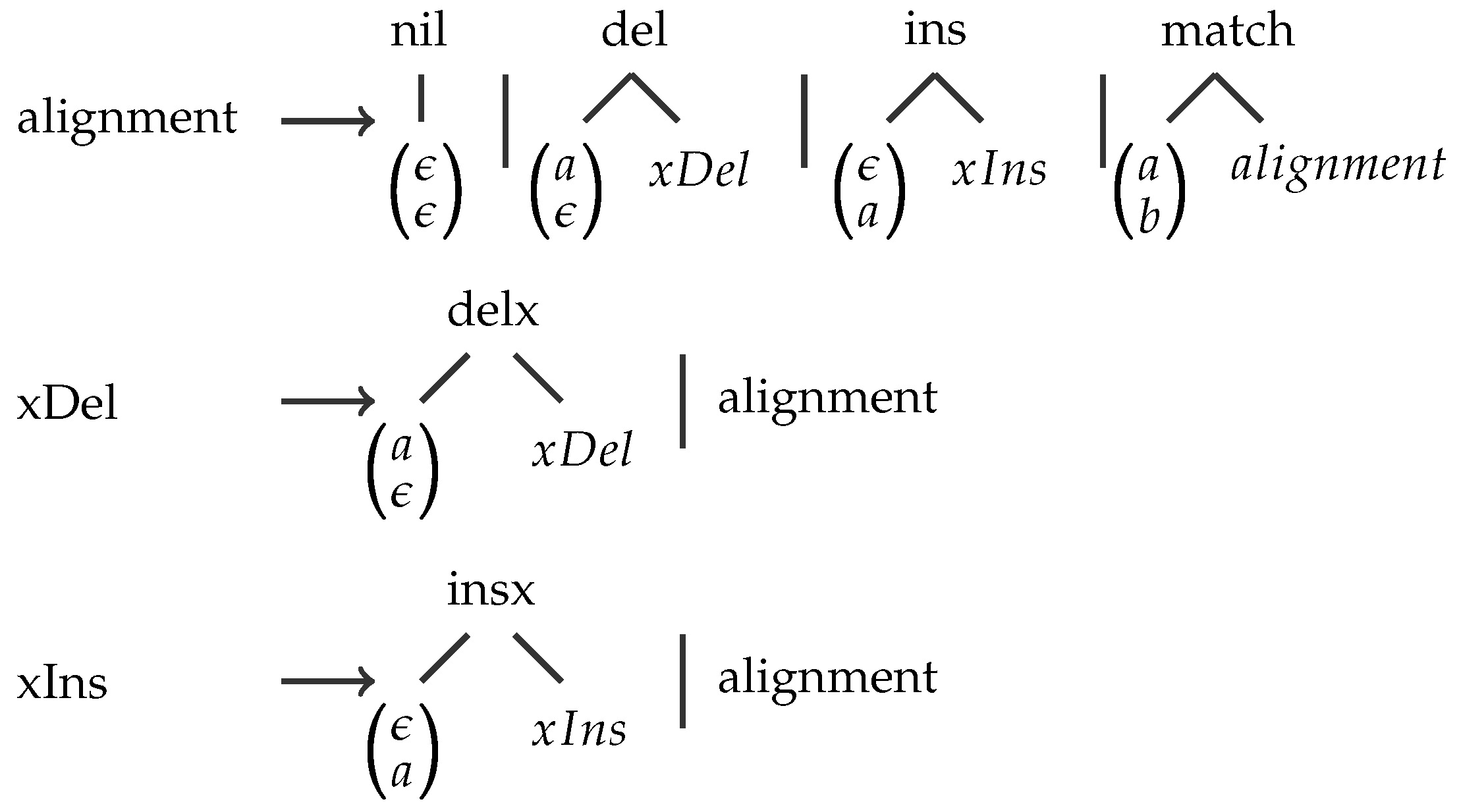
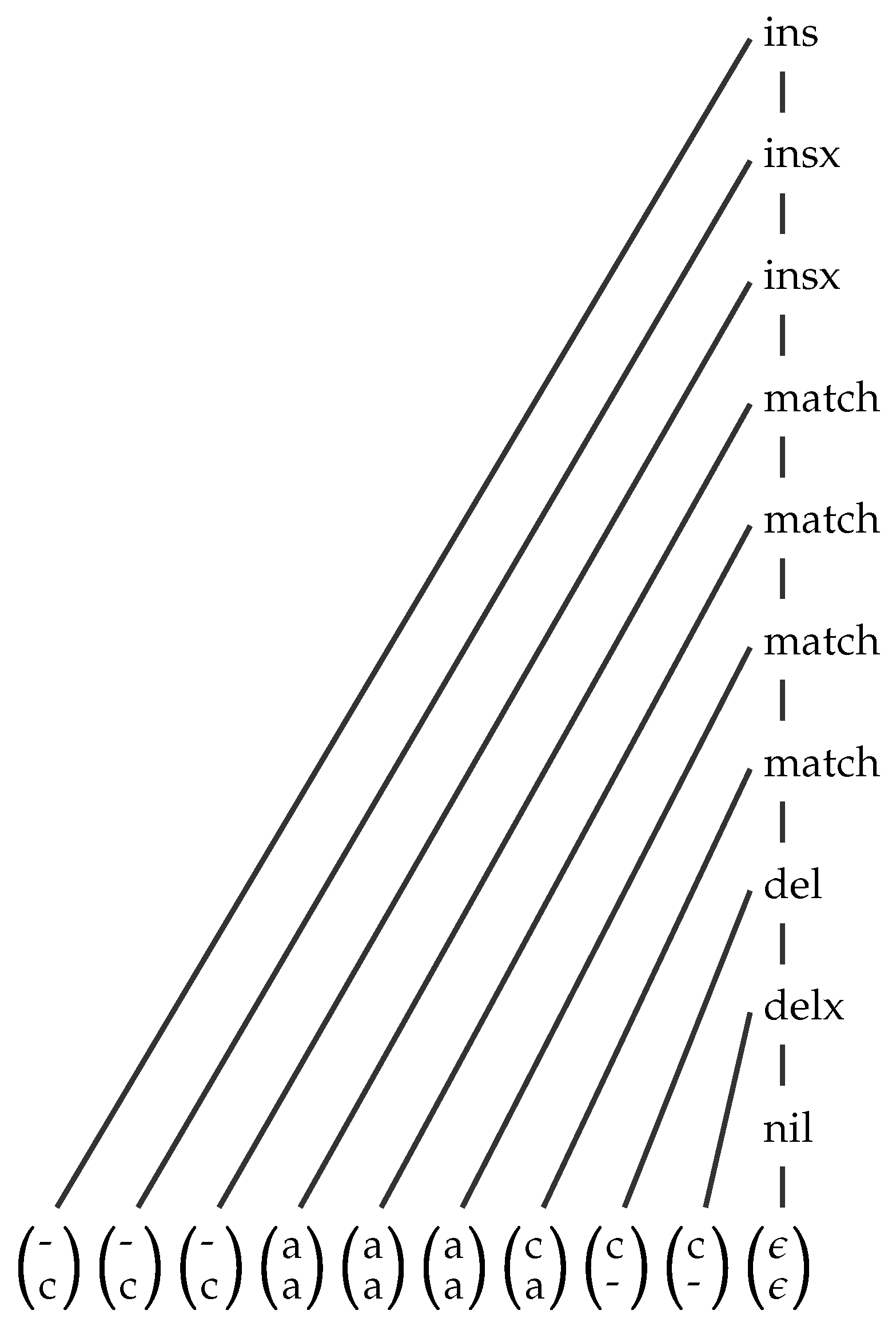
A subproblem of type W can either be decomposed into subproblems of type X and Y, with their scores combined by function f, or its score can be computed by function g from the score of a subproblem of type Z, or it constitutes a base case, where h supplies a default value.
A Simple Example


| Algebra Functions | MATCH | GAP | GOTOH |
|---|---|---|---|
| 0 | 0 | 0 | |
| x | |||
| x | |||
| x | |||
| x | |||
| x | |||
| Choice function | max | min | max |

3. Three Integration Strategies and Their Variants
- NOSORT: Pareto fronts are computed from unsorted lists, by .
- SORT: Lists are sorted on demand, i.e., before computing the Pareto front by .
- EAGER: All of the dynamic programming operations are modified, such that they reduce intermediate results to their Pareto fronts as early as possible. This is called the Pareto-eager strategy.
3.1. Strategy NOSORT
3.2. Strategy SORT
3.3. Sorting Variants within SORT
3.4. Strategy EAGER
3.5. Algorithmic Variants within EAGER
4. Experiments
- Experiment 1: Evaluate the sorting algorithms internal to strategy SORT on random data.
- Experiment 2: Evaluate internal variants of strategy SORT on real-world application data.
- Experiment 3: Evaluate internal variants of strategy EAGER on real-world application data.
- Experiment 4: Evaluate a SORT and an EAGER strategy in search of a separator indicating a strategy switch.
- Experiment 5: Evaluate the relative performance of strategies NOSORT, SORT and EAGER, using the winning internal variants of Experiments 2 and 3.
4.1. Technical Setup
4.2. A Short Description of Tested Bioinformatics Applications
| Application | Name | Dim. | Element Size (Byte) | Dataset |
|---|---|---|---|---|
| RNA Alignment Folding | Ali2D | 2 | 12 | Rfamseed alignments [31] |
| RNA Alignment Folding | Ali3D | 3 | 16 | Rfam seed alignments [31] |
| Gotoh’s algorithm | Gotoh2D | 2 | 8 | BAliBASE3.0 [32] |
| RNA Folding | Fold2D | 2 | 12 | Rfam seed alignments [31] |
| RNA Folding | Fold3D | 3 | 16 | Rfam seed alignments [31] |
| RNA Folding | Prob2D | 2 | 12 | RMDB [33] |
| RNA Folding | Prob4D | 4 | 28 | RMDB [33] |
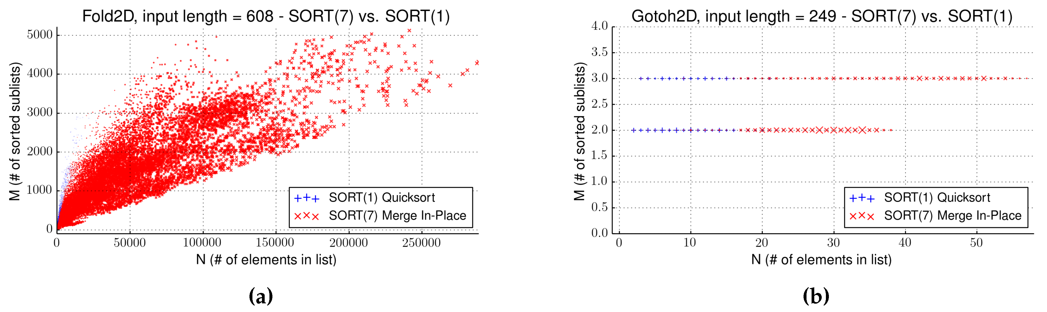
4.3. Evaluation of Strategy SORT
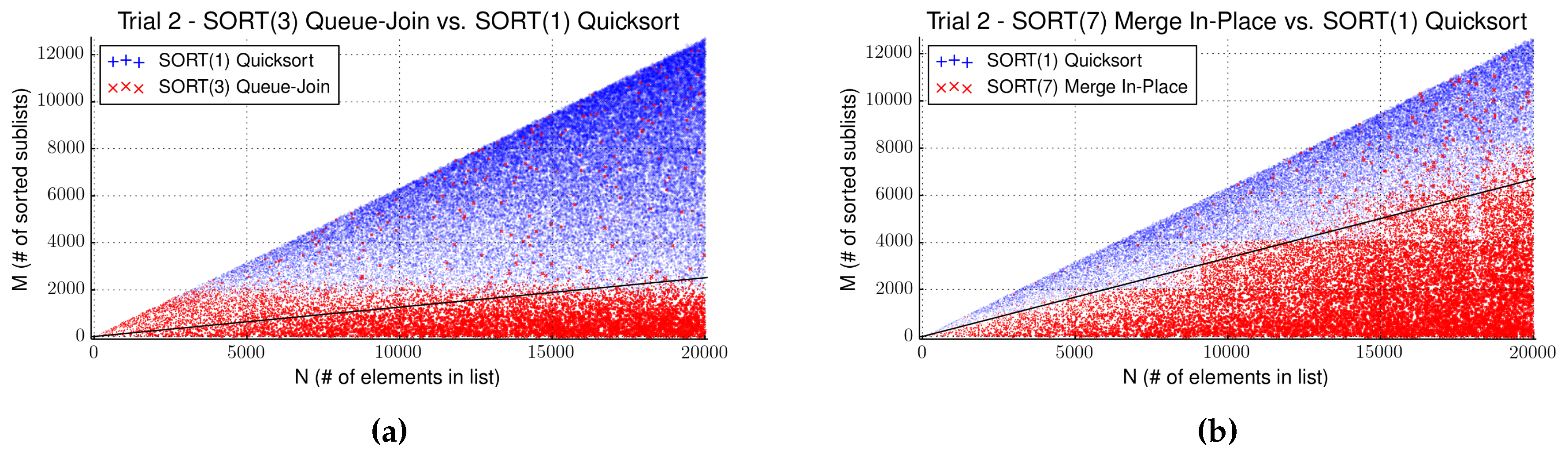
| Algorithm | Avg.Comparator Calls | Max. Saved Time (s) | Separator |
|---|---|---|---|
| Trial 1 | |||
| Algorithm 1 Quicksort | 26,692.7 | ||
| Algorithm 2 List-Join | 1,137,920.0 | - | No significant gain |
| Algorithm 3 Queue-Join | 21,780.1 | 29.0 | Always use Algorithm 3 |
| Algorithm 4 In-Join | 716,920.0 | - | Algorithm 4 never performs consistently better |
| Algorithm 5 Merge A | 18,043.2 | 11.3 | Use Algorithm 5 when |
| Algorithm 6 Merge B | 18,700.0 | 7.8 | Use Algorithm 6 when |
| Algorithm 7 Merge In-Place | 18,043.2 | 13.4 | Use Algorithm 7 when |
| Trial 2 | |||
| Algorithm 1 Quicksort | 222,480.0 | ||
| Algorithm 2 List-Join | 50,668,600.0 | - | No significant gain |
| Algorithm 3 Queue-Join | 181,884.0 | 33.2 | When |
| Algorithm 4 In-Join | 31,480,100.0 | - | Algorithm 4 never performs consistently better |
| Algorithm 5 Merge A | 157,102.0 | 44.9 | Use Algorithm 5 when |
| Algorithm 6 Merge B | 161,502.0 | 28.1 | Use Algorithm 6 when |
| Algorithm 7 Merge In-Place | 157,102.0 | 62.7 | Use Algorithm 7 when |
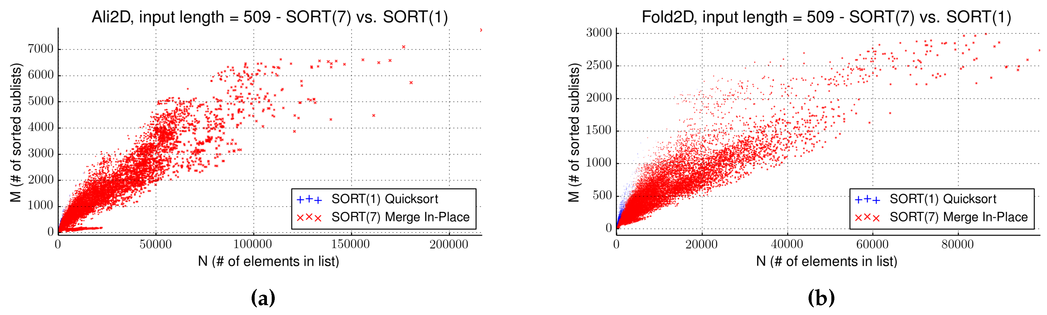
| Name | Input Size | Front Size | Gain (s) | Algorithm | Sort (s) | Pareto (s) | SORT(1) (s) | SORT(7) (s) |
|---|---|---|---|---|---|---|---|---|
| Ali2D | 509 | 487 | 59.1 | Algorithm 7 | 341.9 | 354.5 | 579.77 | 530.0 |
| Gotoh2D | 249 | 209,744 | 0 | Algorithm 7 | 0.1 | 0.1 | 29.42 | 30.3 |
| Fold2D | 509 | 15 | 26.8 | Algorithm 7 | 169.9 | 175.5 | 334.5 | 312.3 |
| Fold2D | 608 | 13 | 304.7 | Algorithm 7 | 1296.1 | 1305.8 | 2220.24 | 1833.3 |
| Prob2D | 185 | 9 | 0 | Algorithm 7 | 2.1 | 2.3 | 3.64 | 3.6 |
| Ali3D | 200 | 446 | 0.1 | Algorithm 7 | 0.3 | 1.2 | 4.97 | 4.88 |
| Fold3D | 404 | 165 | 40.7 | Algorithm 7 | 370.4 | 727.3 | 841.64 | 806.7 |
| Prob4D | 185 | 2327 | 125.1 | Algorithm 7 | 287.0 | 1947.9 | 2556.83 | 2469.8 |

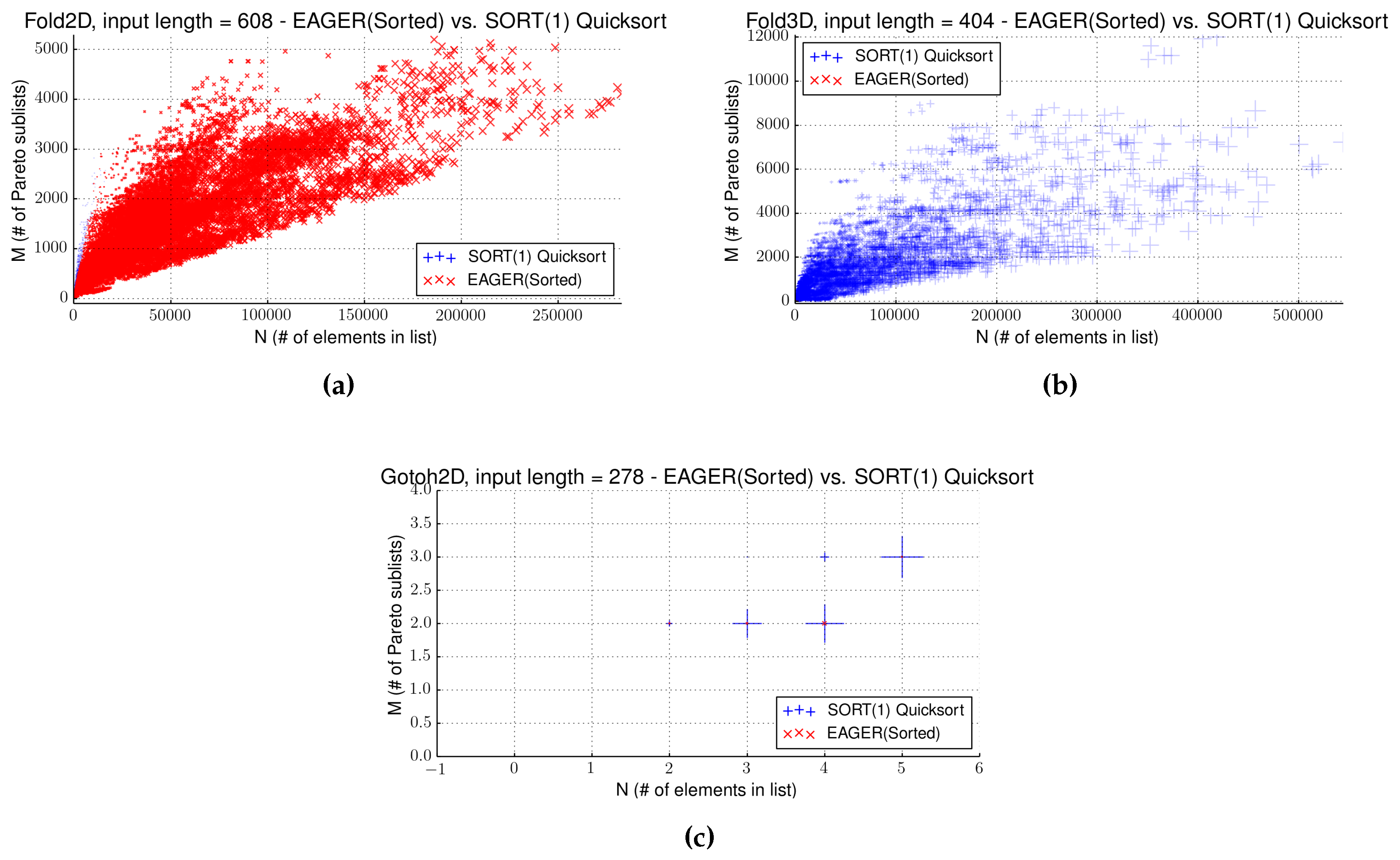
4.4. Strategy EAGER
4.5. Comparing Two Sorting Strategies
| Name | Input Size | Front Size | Gain (s) | Separator | Sort (s) | SORT(1) (s) | EAGER(sort) (s) |
|---|---|---|---|---|---|---|---|
| Ali2D | 509 | 487 | 220.46 | - | 220.1 | 579.77 | 356.11 |
| Gotoh2D | 249 | 209,744 | - | - | 0.1 | 29.42 | 29.83 |
| Fold2D | 608 | 13 | 762.16 | - | 542.3 | 2220.24 | 1054.39 |
| Prob2D | 185 | 9 | 0 | - | 1.7 | 3.64 | 2.76 |
| Ali3D | 200 | 446 | - | - | 4.3 | 4.97 | 8.04 |
| Fold3D | 404 | 165 | - | - | 5757.9 | 841.64 | 5810.36 |
| Prob4D | 185 | 2327 | - | - | 14,442.3 | 2556.83 | 14,552.12 |

4.6. Putting It All Together
| Name | Input | Front | NOSORT | NOSORT(B) | SORT(1) | SORT(7) | EAGER(Sort.) | EAGER(Uns.) |
|---|---|---|---|---|---|---|---|---|
| Ali2D | 509 | 487 | 667.84 | - | 579.77 | 529.98 | 356.11 | 775.77 |
| Gotoh2D | 249 | 209,744 | 29.19 | - | 29.42 | 30.32 | 29.83 | 29.75 |
| Fold2D | 509 | 15 | 154.12 | - | 334.53 | 312.28 | 216.54 | 228.29 |
| Fold2D | 608 | 13 | 631.43 | - | 2220.24 | 1833.31 | 1054.39 | 1279.03 |
| Prob2D | 185 | 9 | 2.05 | - | 3.64 | 3.6 | 2.76 | 2.36 |
| Ali3D | 200 | 446 | 5.43 | 4.93 | 4.97 | 4.88 | 8.04 | 4.85 |
| Fold3D | 404 | 165 | 314.52 | 704.03 | 841.64 | 806.67 | 5810.36 | 813.2 |
| Prob4D | 185 | 2327 | 1774.88 | 1227.13 | 2556.83 | 2449.83 | 14,552.12 | 2535.11 |
4.7. Influence of Search Space Properties and Dimensionality
5. Conclusions
5.1. Using Pareto Products in Bellman’s GAP
- Bellman’s GAP provides a single operator in GAP-L to express Pareto products of evaluation algebras in the form and for higher dimensions as . The compiler can switch between code generation for the two- and the multi-dimensional case.
- Different strategies, NOSORT, NOSORT(B), SORT(1), SORT(7), EAGER (sorted) and EAGER (unsorted), are available via compilation switches. Thus, GAP-L source code does not need to be changed when exploring different strategies.
- If nothing is known about the peculiarities of the application, we recommend to start out with strategy NOSORT. If this does not solve the problem to satisfaction, other strategies should be tried.
5.2. Hand Coding Pareto Optimization into a Dynamic Programming Algorithm
- First of all, consider the possibility of abandoning hand coding and evaluate the suitability of Bellman’s GAP for the purpose. Even when you have already coded the equivalent of and , reformulating your program in ADP will be faster and less error-prone than modifying your source code towards the equivalent of . Doing so, you get a correct Pareto implementation for free. Keep in mind that with hand coding, you also have to implement the backtracing of Pareto-optimal solutions (i.e., the solution candidates behind the Pareto-optimal scores), while Bellman’s GAP also generates the backtracing phase for you.
- Aim first for an implementation of the NOSORT strategy. It is the simplest to implement and was a good choice in most of our test cases.
- Use an abstract data type to interface recurrences and scoring functions.
- Provide separate implementations for evaluating under scoring systems A and B first, and test them thoroughly.
- Then, implement the equivalent of . For debugging, make use of the mathematical fact that the optima under A and B must show up as the extreme points in the Pareto front under .
- If efficiency is problematic and you are going to implement another strategy X, make use of the property that NOSORT and strategy X must produce the identical Pareto fronts on the same input.
- If you choose to implement a sorting strategy, keep in mind our observation that sorting algorithm performance on random data is not meaningful for deciding on its use in the dynamic programming context. Use off-the-shelf Quicksort, or Merge-in-place if memory is critical.
- All dynamic programming with multiple solutions is based on the law of (strict) monotonicity, which all scoring functions must obey. Floating point errors can obstruct this prerequisite with functions that mathematically obey it.
5.3. Outlook
Acknowledgments
Author Contributions
Conflicts of Interest
References
- Branke, J.; Deb, K.; Miettinen, K.; Slowinski, R. (Eds.) Multiobjective Optimization, Interactive and Evolutionary Approaches (Outcome of Dagstuhl Seminars); Lecture Notes in Computer Science; Springer: Berlin, Germany; Heidelberg, Germany, 2008; Volume 5252.
- Goodrich, M.T.; Pszona, P. Two-Phase Bicriterion Search for Finding Fast and Efficient Electric Vehicle Routes. In Proceedings of the 22nd ACM SIGSPATIAL International Conference on Advances in Geographic Information Systems, Dallas, TX, USA, 4–7 November 2014; SIGSPATIAL ’14. ACM: New York, NY, USA, 2014; pp. 193–202. [Google Scholar]
- Müller-Hannemann, M.; Weihe, K. Pareto Shortest Paths Is Often Feasible in Practice. In Algorithm Engineering; Brodal, G., Frigioni, D., Marchetti-Spaccamela, A., Eds.; Lecture Notes in Computer Science; Springer: Berlin, Germany; Heidelberg, Germany, 2001; Volume 2141, pp. 185–197. [Google Scholar]
- Delling, D.; Pajor, T.; Werneck, R.F. Round-Based Public Transit Routing. In Proceedings of the 14th Meeting on Algorithm Engineering and Experiments (ALENEX’12), Society for Industrial and Applied Mathematics, Kyoto, Japan, 16 Jan 2012.
- Rajapakse, J.; Mundra, P. Multiclass gene selection using Pareto-fronts. IEEE/ACM Trans. Comput. Biol. Bioinform. 2013, 10, 87–97. [Google Scholar] [CrossRef] [PubMed]
- Taneda, A. MODENA: A multi-objective RNA inverse folding. Adv. Appl. Bbioinform. Chem. 2011, 4, 1–12. [Google Scholar] [CrossRef]
- Zhang, C.; Wong, A. Toward efficient molecular sequence alignment: A system of genetic algorithm and dynamic programming. Trans. Syst. Man Cybern. B Cybern. 1997, 27, 918–932. [Google Scholar] [CrossRef] [PubMed]
- Bellman, R. Dynamic Programming, 1st ed.; Princeton University Press: Princeton, NJ, USA, 1957. [Google Scholar]
- Cormen, T.H.; Stein, C.; Rivest, R.L.; Leiserson, C.E. Introduction to Algorithms, 2nd ed.; McGraw-Hill Higher Education: Cambridge, MA, USA and London, UK, 2001. [Google Scholar]
- Durbin, R.; Eddy, S.R.; Krogh, A.; Mitchison, G. Biological Sequence Analysis; Cambridge University Press: Cambridge, UK, 1998. [Google Scholar]
- Giegerich, R.; Touzet, H. Modeling Dynamic Programming Problems over Sequences and Trees with Inverse Coupled Rewrite Systems. Algorithms 2014, 7, 62–144. [Google Scholar]
- Getachew, T.; Kostreva, M.; Lancaster, L. A generalization of dynamic programming for Pareto optimization in dynamic networks. Revue Fr. Autom. Inform. Rech. Opér. Rech. Opér. 2000, 34, 27–47. [Google Scholar]
- Sitarz, S. Pareto optimal allocation and dynamic programming. Ann. Oper. Res. 2009, 172, 203–219. [Google Scholar] [CrossRef]
- Schnattinger, T.; Schoening, U.; Marchfelder, A.; Kestler, H. Structural RNA alignment by multi-objective optimization. Bioinformatics 2013, 29, 1607–1613. [Google Scholar] [CrossRef] [PubMed]
- Schnattinger, T.; Schoening, U.; Marchfelder, A.; Kestler, H. RNA-Pareto: Interactive analysis of Pareto-optimal RNA sequence-structure alignments. Bioinformatics 2013, 29, 3102–3104. [Google Scholar] [CrossRef] [PubMed][Green Version]
- Libeskind-Hadas, R.; Wu, Y.C.; Bansal, M.; Kellis, M. Pareto-optimal phylogenetic tree reconciliation. Bioinformatics 2014, 30, i87–i95. [Google Scholar] [CrossRef] [PubMed]
- Giegerich, R.; Meyer, C.; Steffen, P. A discipline of dynamic programming over sequence data. Sci. Comput. Program. 2004, 51, 215–263. [Google Scholar] [CrossRef]
- Zu Siederdissen, C.H. Sneaking around Concatmap: Efficient Combinators for Dynamic Programming. In Proceedings of the 17th ACM SIGPLAN International Conference on Functional Programming, ICFP ’12, Copenhagen, Denmark, 10–12 September 2012; ACM: New York, NY, USA, 2012; pp. 215–226. [Google Scholar]
- Sauthoff, G.; Möhl, M.; Janssen, S.; Giegerich, R. Bellman’s GAP—A Language and Compiler for Dynamic Programming in Sequence Analysis. Bioinformatics 2013, 29, 551–560. [Google Scholar] [CrossRef] [PubMed]
- Sauthoff, G.; Giegerich, R. Yield grammar analysis and product optimization in a domain-specific language for dynamic programming. Sci. Comput. Program. 2014, 87, 2–22. [Google Scholar] [CrossRef]
- Saule, C.; Giegerich, R. Pareto optimization in algebraic dynamic programming. Algorithms Mol. Biol. 2015, 10, 22. [Google Scholar] [CrossRef] [PubMed]
- Graham, R.L.; Knuth, D.E.; Patashnik, O. Concrete Mathematics: A Foundation for Computer Science, 2nd ed.; Addison-Wesley Longman Publishing Co., Inc.: Boston, MA, USA, 1994. [Google Scholar]
- Yukish, M. Algorithms to Identify Pareto Points in Multi-Dimensional Data Sets. Ph.D. Thesis, College of Engineering, Pennsylvania State University, University Park, PA, USA, 2004. [Google Scholar]
- Bentley, J.L. Multidimensional Divide-and-Conquer. Commun. ACM 1980, 23, 214–229. [Google Scholar] [CrossRef]
- Gotoh, O. An Improved Algorithm for Matching Biological Sequences. J. Mol. Biol. 1982, 162, 705–708. [Google Scholar] [CrossRef]
- Sedgewick, R. Implementing Quicksort Programs. Commun. ACM 1978, 21, 847–857. [Google Scholar] [CrossRef]
- Brodal, G.S.; Fagerberg, R.; Moruz, G. On the Adaptiveness of Quicksort. J. Exp. Algorithmics 2008, 12, 3.2:1–3.2:20. [Google Scholar] [CrossRef]
- Dudzinski, K.; Dydek, A. On a Stable Storage Merging Algorithm. Inf. Process. Lett. 1981, 12, 5–8. [Google Scholar] [CrossRef]
- Gatter, T. Integrating Pareto Optimization into the Dynamic Programming Framework Bellman’s GAP. Master’s Thesis, Bielefeld University, Bielefeld, Germany, 2015. [Google Scholar]
- Boost Timer Library. Available online: http://www.boost.org/libs/timer/ (accessed on 18 September 2015).
- Nawrocki, E.P.; Burge, S.W.; Bateman, A.; Daub, J.; Eberhardt, R.Y.; Eddy, S.R.; Floden, E.W.; Gardner, P.P.; Jones, T.A.; Tate, J.; et al. Rfam 12.0: Updates to the RNA families database. Nucleic Acids Res. 2015, 43, D130–D137. [Google Scholar] [CrossRef] [PubMed]
- Thompson, J.D.; Koehl, P.; Poch, O. BAliBASE 3.0: Latest developments of the multiple sequence alignment benchmark. Proteins 2005, 61, 127–136. [Google Scholar] [CrossRef] [PubMed]
- Cordero, P.; Lucks, J.B.; Das, R. An RNA Mapping DataBase for curating RNA structure mapping experiments. Bioinform. 2012, 28, 3006–3008. [Google Scholar] [CrossRef] [PubMed]
- Janssen, S.; Schudoma, C.; Steger, G.; Giegerich, R. Lost in folding space? Comparing four variants of the thermodynamic model for RNA secondary structure prediction. BMC Bioinformatics 2011, 12, 429. [Google Scholar] [CrossRef] [PubMed]
- Xia, T.; SantaLucia, J.J.; Burkard, M.E.; Kierzek, R.; Schroeder, S.J.; Jiao, X.; Cox, C.; Turner, D.H. Thermodynamic parameters for an expanded nearest-neighbor model for formation of RNA duplexes with Watson-Crick base pairs. Biochemistry 1998, 37, 14719–14735. [Google Scholar] [CrossRef] [PubMed]
- Mortimer, S.; Trapnell, C.; Aviran, S.; Pachter, L.; Lucks, J. SHAPE-Seq: High-Throughput RNA Structure Analysis. Curr. Protoc. Chem. Biol. 2012, 4, 275–297. [Google Scholar] [PubMed]
- Loughrey, D.; Watters, K.E.; Settle, A.H.; Lucks, J.B. SHAPE-Seq 2.0: Systematic optimization and extension of high-throughput chemical probing of RNA secondary structure with next generation sequencing. Nucleic Acids Res. 2014, 42. [Google Scholar] [CrossRef] [PubMed]
- Ziehler, W.A.; Engelke, D.R. Probing RNA Structure with Chemical Reagents and Enzymes. Curr. Protoc. Nucleic Acid Chem. 2001. [Google Scholar] [CrossRef]
- Wells, S.E.; Hughes, J.M.; Igel, A.H.; Ares, M.J. Use of dimethyl sulfate to probe RNA structure in vivo. Methods Enzymol. 2000, 318, 479–493. [Google Scholar] [PubMed]
- Talkish, J.; May, G.; Lin, Y.; Woolford, J.L., Jr.; McManus, C.J. Mod-seq: High-throuput sequencing for chemical probing of RNA structure. RNA 2014, 20, 713–720. [Google Scholar] [CrossRef] [PubMed]
- Gardner, P.P.; Giegerich, R. A comprehensive comparison of comparative RNA structure prediction approaches. BMC Bioinform. 2004, 5, 140. [Google Scholar] [CrossRef] [PubMed]
- Saule, C.; Janssen, S. Alternatives in integrating probing data in RNA secondary structure prediction. Manuscript in preparation.
- Hofacker, I.L.; Bernhart, S.H.F.; Stadler, P.F. Alignment of RNA base pairing probability matrices. Bioinformatics 2004, 20, 2222–2227. [Google Scholar] [CrossRef] [PubMed]
- Bernhart, S.; Hofacker, I.L.; Will, S.; Gruber, A.; Stadler, P.F. RNAalifold: improved consensus structure prediction for RNA alignments. BMC Bioinform. 2008, 9, 474. [Google Scholar] [CrossRef] [PubMed]
- Janssen, S.; Giegerich, R. Ambivalent covariance models. BMC Bioinform. 2015, 16, 178. [Google Scholar] [CrossRef] [PubMed]
- Sauthoff, G. Bellman’s GAP: A 2nd Generation Language and System for Algebraic Dynamic Programming. Ph.D. Thesis, Bielefeld University, Bielefeld, Germany, 2011. [Google Scholar]
© 2016 by the authors; licensee MDPI, Basel, Switzerland. This article is an open access article distributed under the terms and conditions of the Creative Commons by Attribution (CC-BY) license (http://creativecommons.org/licenses/by/4.0/).
Share and Cite
Gatter, T.; Giegerich, R.; Saule, C. Integrating Pareto Optimization into Dynamic Programming. Algorithms 2016, 9, 12. https://doi.org/10.3390/a9010012
Gatter T, Giegerich R, Saule C. Integrating Pareto Optimization into Dynamic Programming. Algorithms. 2016; 9(1):12. https://doi.org/10.3390/a9010012
Chicago/Turabian StyleGatter, Thomas, Robert Giegerich, and Cédric Saule. 2016. "Integrating Pareto Optimization into Dynamic Programming" Algorithms 9, no. 1: 12. https://doi.org/10.3390/a9010012
APA StyleGatter, T., Giegerich, R., & Saule, C. (2016). Integrating Pareto Optimization into Dynamic Programming. Algorithms, 9(1), 12. https://doi.org/10.3390/a9010012