Generating Realistic Labelled, Weighted Random Graphs ^†

Abstract

Generative algorithms for random graphs have yielded insights into the structure and evolution of real-world networks. Most networks exhibit a well-known set of properties, such as heavy-tailed degree distributions, clustering and community formation. Usually, random graph models consider only structural information, but many real-world networks also have labelled vertices and weighted edges. In this paper, we present a generative model for random graphs with discrete vertex labels and numeric edge weights. The weights are represented as a set of Beta Mixture Models (BMMs) with an arbitrary number of mixtures, which are learned from real-world networks. We propose a Bayesian Variational Inference (VI) approach, which yields an accurate estimation while keeping computation times tractable. We compare our approach to state-of-the-art random labelled graph generators and an earlier approach based on Gaussian Mixture Models (GMMs). Our results allow us to draw conclusions about the contribution of vertex labels and edge weights to graph structure.

1. Introduction

Network analysis is concerned with finding patterns and anomalies in real-world graphs, such as social networks, computer and communication networks, or biological and ecological processes. Real graphs exhibit a number of interesting structural and evolutionary properties, such as the formation of a giant component, heavy-tailed degree distribution, small diameter, shrinking diameter, and the Densification Power Law (DPL) [1,2,3,4,5].

Besides discovering network properties, researchers are interested in the mechanisms of network formation. Generative graph models provide an abstraction of how graphs form: if the model is accurate, generated graphs will obey the same properties as real graphs. Generated graphs are also useful for simulation experiments, hypothesis testing and making predictions about graph evolution or missing graph elements. Most generative models are for unlabelled, unweighted graphs [1,3,4,6,7], although a few models take discrete vertex labels into account [8,9,10].

In this paper, we develop a generative model for labelled, weighted graphs. Weights are commonly used to represent the number of occurrences of each edge: e-mails sent between individuals in a social network [11]; calls to a subroutine in a software call graph [12]; or people walking between a pair of sensors in a building access control network [13]. In other applications, the edge weight may represent continuous values: donation amounts in a bipartite graph of donors and political candidates [11]; distance or speed in a transportation network [12]; or elapsed time to walk between the sensors in the building network [13]. In some cases, the weight has more than one dimension [12,13].

Our main motivation for this work is to create “realistic” random graphs for evaluating graph mining algorithms. Some interesting graph datasets are very small; our approach can generate large graphs with the same characteristics as a smaller input graph. Random graphs can also ameliorate concerns about privacy. A second motivation is to better understand the laws governing the relationship between graph structure and attributes. Our experiments show the extent to which various graph properties are related to labels and weights.

Our model, Agwan (Attribute Graph: Weighted and Numeric), represents the distribution of edge weights as Beta Mixture Models (BMMs) which are learned from weighted input graphs. Learning BMM parameters using Bayesian estimation is analytically intractable. Numerical solutions to simulate the posterior distribution are available, but these incur high computational cost. In Section 3, we introduce an approximation to the prior/posterior distribution of the parameters in the beta distribution and propose an analytically tractable (closed-form) Bayesian approach to parameter estimation, based on the Variational Inference (VI) framework. Following the principles of VI and utilizing the relative convexity bound, the extended factorised approximation method is applied to approximate the distribution of the BMM parameters. In a fully Bayesian model where all the parameters of the BMM are considered as variables and assigned proper distributions, our approach can asymptotically find the optimal estimate of the parameters of the posterior distribution. In addition, the model complexity depends on the empirical distribution of the data. A closed-form solution is proposed to avoid the need for numerical methods in each iteration. Our approach avoids the drawback of overfitting, as in the conventional Expectation Maximisation (EM) algorithm.

This paper is arranged as follows: Section 2 is an overview of generative graph models and approaches to estimating mixture model parameters; Section 3 presents Agwan, our generative model for weighted and numeric labelled graphs, including our algorithm for fitting Agwan’s parameters to real input graphs. Section 4 gives an overview of the datasets used in the experiments, and outlines the statistical measures and tests used to evaluate the generated graphs. The experiments in Section 5 demonstrate that the vertex labels and edge weights of a graph can predict the graph structure with high accuracy. Conclusions are in Section 6.

2. Related Work

Our understanding of the mathematical properties of graph structure was pioneered by Paul Erdős and Alfréd Rényi [3]. Graph formation is modelled as a Bernoulli process, parameterised by the number of vertices and a wiring probability between each vertex pair. While it has been essential to our understanding of component sizes and expected diameter, the Erdős-Rényi model does not explain other important properties of real-world graphs such as degree distribution, transitivity and clustering [2,5].

Barabási and Albert’s Preferential Attachment model [1] uses the “rich get richer” principle to grow graphs from a few vertices up to the desired size. The probability of an edge is proportional to the number of edges already connected to a vertex. This generates graphs with power-law degree distributions. A number of variants of Preferential Attachment have been proposed [2,5]. Still, Preferential Attachment models lack some desired properties, such as community structure.

The RMat algorithm [6] solves the community structure problem with its recursive matrix approach. RMat graphs consist of $2^n$ vertices and E edges, with four probabilities $a,b,c,d$ to determine in which quadrant of the adjacency matrix each edge falls. These parameters allow the specification of power-law or log-normal degree distributions; if $a=b=c=d$, the result will be an Erdős-Rényi graph.

Kronecker Graphs [7] fulfil all the properties mentioned above, as well as the DPL (Densification Power Law) and shrinking diameter effect. The model starts with an initiator matrix. Kronecker multipication is recursively applied to yield the final adjacency matrix of the desired size. This work synthesises the previous work in random graphs in a very elegant way and proves that RMat graphs are a special case of Stochastic Kronecker graphs.

The models above tend to have a small number of parameters and are analytically tractable, with simple and elegant proofs of the desired properties. However, graph labels are not taken into consideration. Stochastic models are another class of generative algorithm which may not be amenable to analytical proofs but can be fit to real-world labelled graphs and used to learn the properties of those graphs. Models in this category include the Stochastic Block Model [10] and Latent Space approaches [8].

The Multiplicative Attribute Graph (MAG) model [9] draws on both of the above strands of research. MAG is parameterised by the number of vertices, a set of prior probabilities for vertex label values and a set of affinity matrices specifying the probability of an edge conditioned on the vertex labels. The affinity matrices can be learned from real graphs using Maximum Likelihood Estimation [14]. [9] proves that Kronecker Graphs are a special case of MAG graphs, and that suitably-parameterised MAG graphs fulfil all the desired properties: log-normal or power-law degree distribution, small diameter, the existence of a unique giant component and the DPL. However, the MAG model can only generate unweighted graphs. We believe that our method, described in the next section, is the first generative model for labelled, weighted graphs.

The Agwan model requires a suitable probability distribution to model the edge weights accurately and efficiently. The Gaussian distribution is popular as it has an analytically tractable Probability Density Function (PDF); a weighted mixture of Gaussian components provides a reasonable approximation to any general probability distribution [15]. The resulting Gaussian Mixture Model (GMM) is quite flexible and is used extensively in statistical pattern recognition [16]. If the number of mixture components is known in advance, the GMM parameters can be estimated using EM (Expectation Maximisation) [17]. However, if the number of mixtures is unknown, EM can result in overfitting. The problem of knowing the “correct” number of components can be avoided by using a non-parametric model: the approach in [18] assumes an infinite number of components and uses VI (Variational Inference) to determine the optimal number for a given dataset. The variational algorithm can be accelerated for higher-dimensional data using a kd-tree [19].

In [20], the edge weight parameters are specified as a GMM. However, the Gaussian distribution may not be the best choice where the weight is a countable quantity representing the number of occurrences of an edge. In this case, the weights are bounded by $(0,+\infty )$, while the Gaussian distribution is bounded by $(-\infty ,+\infty )$. Although the weights can be modelled as a GMM, a large number of mixture components are required to describe the data close to the boundary [21]. Alternatives to the GMM include the truncated GMM [21] and the BMM [22]. We investigate these options in this paper.

The most central task in modeling the data with a BMM is parameter estimation. Since the normalisation constant (the beta function) in the beta distribution is defined as a fraction of integrals, it is difficult to obtain a closed-form expression for estimating the parameters. For maximum likelihood estimation of the BMM parameters, [23,24] proposed an EM algorithm [25], with iterative numerical calculations in the maximisation step. As with GMMs, the EM algorithm for BMM has some disadvantages: it can lead to overfitting when the mixture models are excessively complex; and the iterative numerical calculation in the maximisation step (e.g., with the Newton-Raphson method) has a high computational cost.

For Bayesian estimation, we can formally find the prior distribution and the conjugate posterior distribution of the parameters of the beta distribution. However, this posterior distribution is still defined with an integration expression in the denominator such that the closed-form of the posterior distribution is analytically intractable. [22] proposed a practical Bayesian estimation algorithm based on the Gibbs sampling method, which simulates the posterior distribution approximately rather than computing it. This method prevents the overfitting problem but still suffers from high computational cost because of the Gibbs sampling, especially when the data is in a high-dimensional space. To overcome this problem, [26,27] proposed a full Bayesian estimation method for parameter estimation in a BMM, where the VI framework was employed and an analytically tractable solution can be obtained. The proposed method facilitates the parameter estimation.

3. Agwan: A Generative Model for Labelled, Weighted Graphs

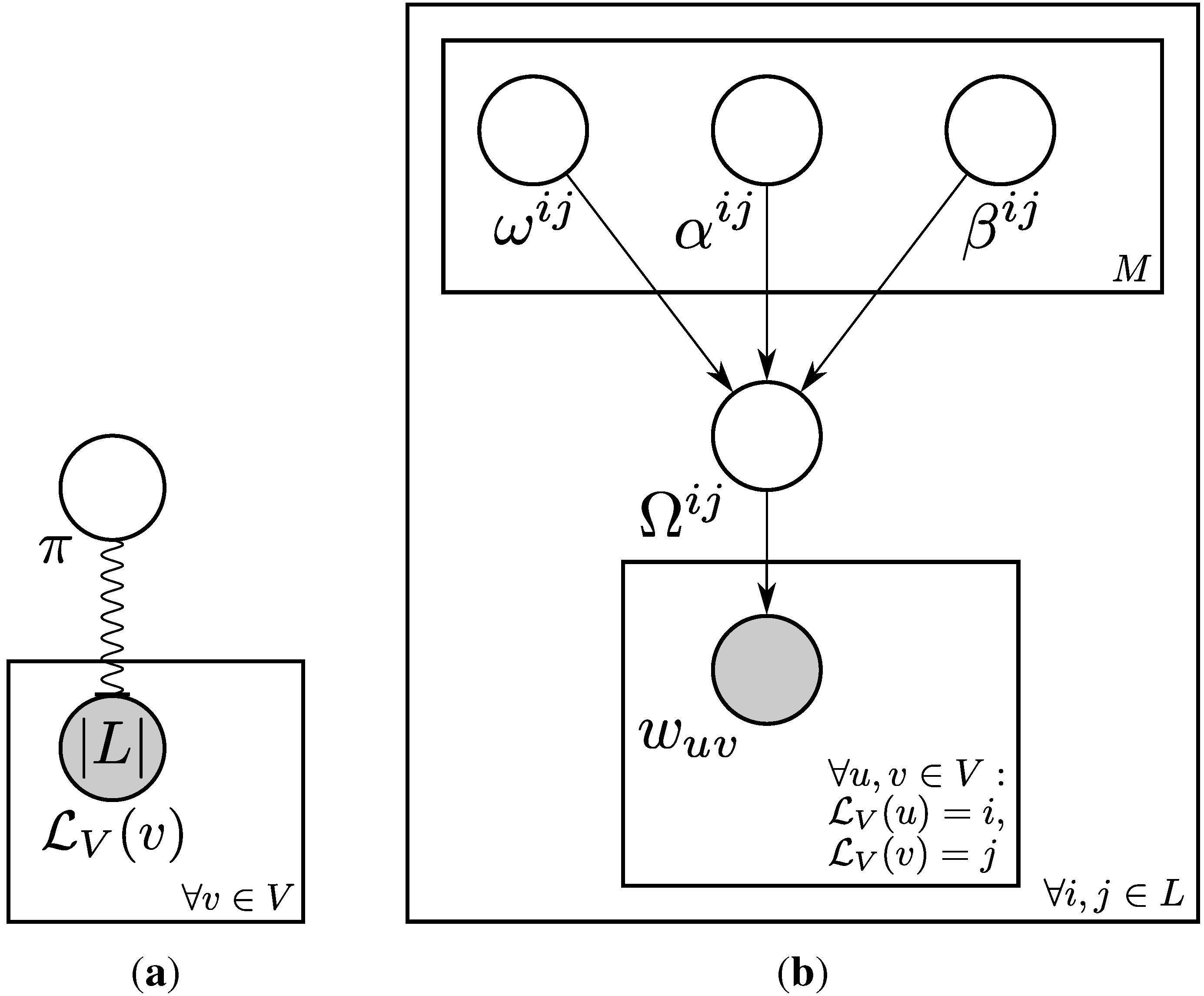
In this section, we present our generative model, Agwan (Attribute Graph: Weighted and Numeric). The model is illustrated in Figure 1.

Figure 1. Agwan parameters. (a) Vertex Labels; (b) Edge Weights.

Figure 1. Agwan parameters. (a) Vertex Labels; (b) Edge Weights.

Consider a graph $G=(V,E)$ with discrete vertex label values drawn from a set L (Figure 1a). For each combination of vertex attributes $〈i,j〉$, the corresponding mixture model ${\Omega }^{ij}$ parameterises the distribution of edge weights, with an edge weight of 0 indicating no edge (Figure 1b). $u,v\in V$ are vertices and $w_{uv},w_{vu}\in \mathbb{N}$ are edge weights. Edges $e\in E$ are specified as a 3-tuple $〈u,v,w_{uv}〉$. Thus, the Agwan model is parameterised by π, the set of prior probabilities over L; and the set of edge weight mixture parameters $\Theta =\left\{{\Omega }^{ij}\right|i,j\in L\}$. For directed graphs, $|\Theta |={\left|L\right|}^2$ and we need to generate both $w_{uv}$ and $w_{vu}$. For undirected graphs, ${\Omega }^{ij}={\Omega }^{ji}$, so $|\Theta |=O\left(\right|L{|}^2/2)$ and $w_{vu}=w_{uv}$.

${\Omega }^{ij}$ is specified as a BMM:

$$\begin{array}{c}\hfill {\Omega }^{ij}=\sum _{m=1}^M{\omega }_m^{ij}·\mathrm{Beta}(a_m^{ij},b_m^{ij})\end{array}$$

(1)

where ${\omega }_m^{ij}$ is the weight of each component; and $\mathrm{Beta}(a_m^{ij},b_m^{ij})$ is the beta distribution with shape parameters $(a_m^{ij},b_m^{ij})$. The PDF of the beta distribution is:

$$\mathrm{Beta}(x;a,b)=\frac{1}{\mathrm{beta}(a,b)}{x}^{a-1}{(1-x)}^{b-1},a,b>0$$

(2)

where $\mathrm{beta}(a,b)$ is the beta function $\mathrm{beta}(a,b)=\frac{\Gamma \left(a\right)\Gamma \left(b\right)}{\Gamma (a+b)}$ and $\Gamma (·)$ is the gamma function defined as $\Gamma \left(z\right)={\int }_0^{\infty }{t}^{z-1}{e}^{-t}dt$. As the support of the BMM is $(0,1)$, we use a constant $s^{ij}$ to scale the data into this range before fitting the BMM parameters. During graph generation, we draw values from the BMM and multiply by $s^{ij}$.

We specify ${\Omega }^{ij}$ such that the weight of the first component ($m=0$) encodes the probability of no edge: ${\omega }_0^{ij}=1-P\left(e_{ij}\right)$, where $P\left(e_{ij}\right)$ is the probability of an edge between pairs of vertices with labels $〈i,j〉$ and is learned from the input graph. The weights of the BMM components ($m\in [1,M]$) are normalised by $P\left(e_{ij}\right)$, so the weights of all the components form a probability distribution: ${\sum }_{m=0}^M{\omega }_m^{ij}=1$.

3.1. Graph Generation

Algorithm 1 describes how to generate a random graph using Agwan($N,L,\pi ,\Theta$). The number of vertices in the generated graph is specified by N. After assigning discrete label values to each vertex (lines 2–3), the algorithm checks each vertex pair $〈u,v〉$ for the occurrence of an edge (lines 4–7). If there is an edge, we assign its weight from mixture component m (lines 8,9). The generated graph is returned as $G=(V,E)$.

Algorithm 1 Agwan Graph Generation

Require:  N (no. of vertices), L (set of discrete label values), π (prior distribution over L), $\Theta =\left\{{\Omega }^{ij}\right\}$ (set of mixture models) 1: Create vertex set V of cardinality N, edge set $E=\varnothing$ 2: for all $u\in V$ do 3:     Randomly draw discrete label $l_u\in L$ according to prior π 4: for all $u,v\in V:u\ne v$ do 5:     $i=l_u,j=l_v$ 6:     Randomly draw mixture component m according to mixture weights ${\omega }^{ij}$ 7:     if $m\ne 0$ then 8:         Randomly draw edge weight $w_{uv}$ from $s^{ij}·\mathrm{Beta}(a_m^{ij},b_m^{ij})$ 9:         Create edge $e=〈u,v,w_{uv}〉,E=E\cup \left\{e\right\}$ 9: return $G=(V,E)$

3.2. Parameter Fitting

To create realistic random graphs, we need to learn the parameters $\pi ,\Theta$ from a real-world input graph G. For each $i,j\in V$, the edge weights $W^{ij}=\left\{w_{ij}\right\}$ follow an unknown, arbitrary probability distribution. For each set of edge weights $W^{ij}$, we choose the scaling parameter $s^{ij}\ge {max}_{W^{ij}}$, then estimate the BMM parameters for the empirical distribution $\raisebox{1ex}{$1$}\!\left/ \!\raisebox{-1ex}{$s^{ij}$}\right.·W^{ij}$, which has support $(0,1]$.

In this section, we describe the Bayesian estimation of BMMs within a VI framework, followed by our algorithms for Agwan parameter fitting.

The beta distribtion has a conjugate prior in the exponential family. The conjugate prior density function can be written as [15,28]:

$$f(a,b)=\frac{1}{C({\alpha }_0,{\beta }_0,{\nu }_0)}{\left[\frac{\Gamma (a+b)}{\Gamma \left(a\right)\Gamma \left(b\right)}\right]}^{{\nu }_0}{e}^{-{\alpha }_0(a-1)}{e}^{-{\beta }_0(b-1)}$$

(3)

where ${\alpha }_0$, ${\beta }_0$, ${\nu }_0$ are free positive parameters and $C({\alpha }_0,{\beta }_0,{\nu }_0)$ is a normalisation factor such that ${\int }_0^{\infty }{\int }_0^{\infty }f(a,b)dadb=1$. Then, we obtain the posterior distribution of $a,b$ as (with N independent and identically distributed (i.i.d.) scalar observations $X=\{x_1,\dots ,x_N\}$)

$$\begin{array}{cc}& f(a,b|X)=\frac{f\left(X\right|a,b\left)f\right(a,b)}{{\int }_0^{\infty }{\int }_0^{\infty }f\left(\mathrm{X}\right|a,b)f(a,b)dadb}\hfill \\ & =\frac{1}{C({\alpha }_N,{\beta }_N,{\nu }_N)}{\left[\frac{\Gamma (a+b)}{\Gamma \left(a\right)\Gamma \left(b\right)}\right]}^{{\nu }_N}{e}^{-{\alpha }_N(a-1)}{e}^{-{\beta }_N(b-1)}dadb\hfill \end{array}$$

(4)

where ${\nu }_N={\nu }_0+N$, ${\alpha }_N={\alpha }_0-{\sum }_{n=1}^{N}ln{x}_n$ and ${\beta }_N={\beta }_0-{\sum }_{n=1}^{N}ln(1-x_n)$. To avoid infinity in the practical implementation, we assign ${\epsilon }_1$ to $x_n$ when $x_n=0$ and $1-{\epsilon }_2$ to $x_n$ when $x_n=1$, where ${\epsilon }_1$ and ${\epsilon }_2$ are slightly positive real numbers.

We introduce an approximation to both the conjugate prior and the posterior distributions of the beta distribution and attempt to solve the Bayesian estimation problem via the factorised approximation method. A distribution can be used as the factorised distribution of the true posterior distribution if the optimal solution to this factorised distribution has exactly the same form as its initialisation. This requirement guarantees that the estimation works iteratively. With the non-negative property of the parameters in the beta distribution and assuming that a and b are statistically independent, we could use some well-defined distribution with support $(0,+\infty )$ to approximate the conjugate prior. One possible way is to assign the gamma distribution to a and b as:

$$\begin{array}{cc}\hfill f(a;\mu ,\alpha )=& \frac{{\alpha }^{\mu }}{\Gamma \left(\mu \right)}{a}^{\mu -1}{e}^{-\alpha a};f(b;\nu ,\beta )=\frac{{\beta }^{\nu }}{\Gamma \left(\nu \right)}{b}^{\nu -1}{e}^{-\beta b}\hfill \end{array}$$

(5)

The conjugate prior is then approximated as:

$$f(a,b)\approx f\left(a\right)f\left(b\right)$$

(6)

The same form of approximation applies to the posterior distribution as:

$$f(a,b|\mathbf{X})\approx f(a\left|\mathbf{X}\right)f\left(b\right|\mathbf{X})$$

(7)

For each observation ${\mathbf{x}}_n$, the corresponding ${\mathbf{z}}_n={[z_{n1},\dots ,z_{nM}]}^T$ is the indication vector defined with respect to the M components in the mixture model. One element of $z_n$ will be equal to 1 and the rest equal to 0, to indicate which mixture component $z_n$ belongs to. Denoting $Z=\{z_1,\dots ,z_N\}$ and assuming the indication vectors are independent given the mixing coefficients, the conditional distribution of $Z$ given $P$ is:

$$\begin{array}{c}\hfill f\left(Z\right|P)=\prod _{n=1}^N\prod _{m=1}^M{p}_m^{z_{nm}}\end{array}$$

(8)

Introducing the Dirichlet distribution as the prior distribution of the mixing coefficients, the probability function of $P$ can be written as:

$$\begin{array}{cc}\hfill f\left(P\right)& =Dir\left(p\right|c)=C\left(\mathbf{c}\right)\prod _{m=1}^M{p}_m^{c_m-1}\hfill \end{array}$$

(9)

where $C\left(\mathbf{c}\right)=\frac{\Gamma \left(\widehat{c}\right)}{\Gamma \left(c_1\right)\cdots \Gamma \left(c_M\right)}$ and $\widehat{c}={\sum }_{m=1}^M{c}_m$. We consider the observation ${\mathbf{x}}_n$ and the unobserved indication vector ${\mathbf{z}}_n$ as the complete data. The conditional distribution of $\mathit{X}=\{{\mathbf{x}}_1,\dots ,{\mathbf{x}}_N\}$ and $\mathit{Z}=\{{\mathbf{z}}_1,\dots ,{\mathbf{z}}_N\}$ given the latent variables $\{\mathit{A},\mathit{B},\mathit{P}\}$ is:

$$\begin{array}{cc}& f(\mathbf{X},\mathbf{Z}|\mathbf{A},\mathbf{B},\mathbf{P})\hfill \\ \hfill =& f\left(\mathbf{X}\right|\mathbf{A},\mathbf{B},\mathbf{P},\mathbf{Z}\left)f\right(\mathbf{Z}\left|\mathbf{P}\right)\hfill \\ \hfill =& f\left(\mathbf{X}\right|\mathbf{A},\mathbf{B},\mathbf{Z}\left)f\right(\mathbf{Z}\left|\mathbf{P}\right)\hfill \\ \hfill =& \prod _{n=1}^N\prod _{m=1}^M{\left[p_m\mathbf{Beta}\left({\mathbf{x}}_n\right|{\mathbf{a}}_m,{\mathbf{b}}_m)\right]}^{z_{nm}}\hfill \end{array}$$

(10)

The algorithm for Bayesian estimation of a BMM model is presented in Algorithm 2. An overview of the derivation of the algorithm from Equations (5)–(10) can be found in Appendix A. For full details of the derivations, refer to [26].

Algorithm 2 Bayesian estimation of a Beta Mixture Model (BMM)

Require:  Number of components M, initial parameters for the Dirichlet distribution, initial parameters (element-wise) ${\alpha }_0>0$, ${\beta }_0>0$, ${\mu }_0>0.6156$, ${\nu }_0>0.6156$. Select initial parameters such that ${\mu }_0/{\alpha }_0>1$ and ${\nu }_0/{\beta }_0>1$. 1: Initialise $r_{nm}$ with k-means 2: Calculate the initial guess of $\overline{a}$ and $\overline{v}$ from ${\alpha }_0,{\beta }_0,{\mu }_0,{\nu }_0$ 3: repeat 4:     Update the hyperparameters $c_m^{*}$, ${\mu }_{lm}^{*}$, ${\alpha }_{lm}^{*}$, ${\nu }_{lm}^{*}$ and ${\beta }_{lm}^{*}$ 5: until convergence     return the current estimated hyperparameters

After initialisation (lines 1,2), Algorithm 2 iterates until the the current estimated model and the previous estimated model are sufficiently close (lines 3–5). The order of updating (line 4) does not matter, but each hyperparameter should be updated exactly once during each iteration. Refer to Appendix A for details of how the intermediate quantities are calculated ($c_m^{*}$ is updated following Equation (A3), ${\mu }_{lm}^{*}$ from Equation (A4), ${\alpha }_{lm}^{*}$ from Equation (A5), ${\nu }_{lm}^{*}$ from Equation (A6) and ${\beta }_{lm}^{*}$ from Equation (A7). The expectations for these quantities are given in Equation (A8).) The algorithm returns the current estimated hyperparameters at the last iteration, which are used to get the approximating posterior distribution. The joint posterior distribution of $a_{lm},b_{lm}$ (Equation (4)) is approximated by the product of two gamma distributions with parameters ${\mu }_{lm}^{*},{\alpha }_{lm}^{*}$ and ${\nu }_{lm}^{*},{\beta }_{lm}^{*}$ (Equations (5) and (7)).

Agwan parameter fitting is performed by Algorithm 3. First, we estimate the vertex label priors (lines 1–3); Next, we sample the edge weights for each possible combination of vertex label values (lines 5–10); The proportion of non-edges is used to estimate the weight of mixture 0 (line 10). We estimate each scaled BMM ${\Omega }^{ij}$ from the appropriate set of samples $W^{ij}$ using Algorithm 2 as described above (lines 12–13). Finally, the mixture weights ${\omega }_m^{ij}$ are normalised so that they sum to 1 (line 14).

Algorithm 3 Agwan Parameter Fitting

Require:  Input graph $G=(V,E)$ 1: $L=\left\{\mathrm{discrete}\mathrm{vertex}\mathrm{label}\mathrm{values}\right\},d=\left|L\right|$ 2: Calculate vertex label priors, apply Laplace smoothing $\forall l\in L:P\left(l\right)=\frac{count\left(l\right)+\alpha }{N+\alpha d}$ 3: $\pi =$ the normalised probability distribution over L such that ${\sum }_{i=1}^{d}P\left(l_i\right)=1$ 4: $\forall i,j\in L:W^{ij}=\varnothing$ 5: for all $u,v\in V:u\ne v$ do 6:     $i=l_u,j=l_v$ 7:     if $〈u,v〉\in E$ then 8:         $W^{ij}=W^{ij}\cup \left\{w_{uv}\right\}$ 9:     else 10:         Increment ${\omega }_0^{ij}$ 11: for all $i,j\in L$ do 12:     ${\omega }_0^{ij}=1-P\left(e_{ij}\mathrm{exists}\right)$ 13:     $s^{ij}={max}_{W^{ij}}$ 14:     $\mathrm{estimate}{\Omega }^{ij}\mathrm{from}\raisebox{1ex}{$1$}\!\left/ \!\raisebox{-1ex}{$s^{ij}$}\right.·W^{ij}\mathrm{using}\mathrm{Algorithm}2$ 15:     Normalise all ${\omega }_m^{ij}$   return $\pi ,\Theta =\left\{{\Omega }^{ij}\right\}$

3.3. Extending Agwan to Multiple Attributes

Agwan can be extended to multiple numeric edge labels by generalising the concept of edge weight to K dimensions. In this case, the weight is parameterised as the multivariate beta distribution. For any random vector x consisting of K elements, the dependencies among the elements $x_1,\dots ,x_K$ can be represented by a mixture model, even if each specific mixture component can only generate vectors with statistically independent elements. Therefore, we define the multivariate BMM as:

$$\begin{array}{c}\hfill f(x;P,A,B)=\sum _{m=1}^M{p}_m·\mathrm{Beta}(x;a_m,b_m)=\sum _{m=1}^M{p}_m·\prod _{k=1}^K\mathrm{Beta}(x_k;a_{km},b_{km})\end{array}$$

(11)

where $x=\{x_1,\dots ,x_K\},P=\{p_1,\dots ,p_M\},A=\{a_1,\dots ,a_M\}$ and $B=\{b_1,\dots ,b_M\}$. $a_m,b_m$ denote the parameter vectors of the m^th mixture component and $a_{km},b_{km}$ are the (scalar) parameters of the beta distribution for element $x_k$. Using this representation, we can apply Algorithm 2 to K-dimensional edge weights.

4. Experimental Section

We evaluate our approach by comparing Agwan with the state-of-the-art in labelled graph generation, represented by the MAG model [9,14]. Agwan and MAG parameters are learned from real-world graphs. We generate random graphs from each model and calculate a series of statistics on each graph. As MAG does not generate weighted graphs, we fixed the weight of the edges in the generated graphs to the mean edge weight from the input graphs. This ensures that statistics such as average vertex strength are maintained.

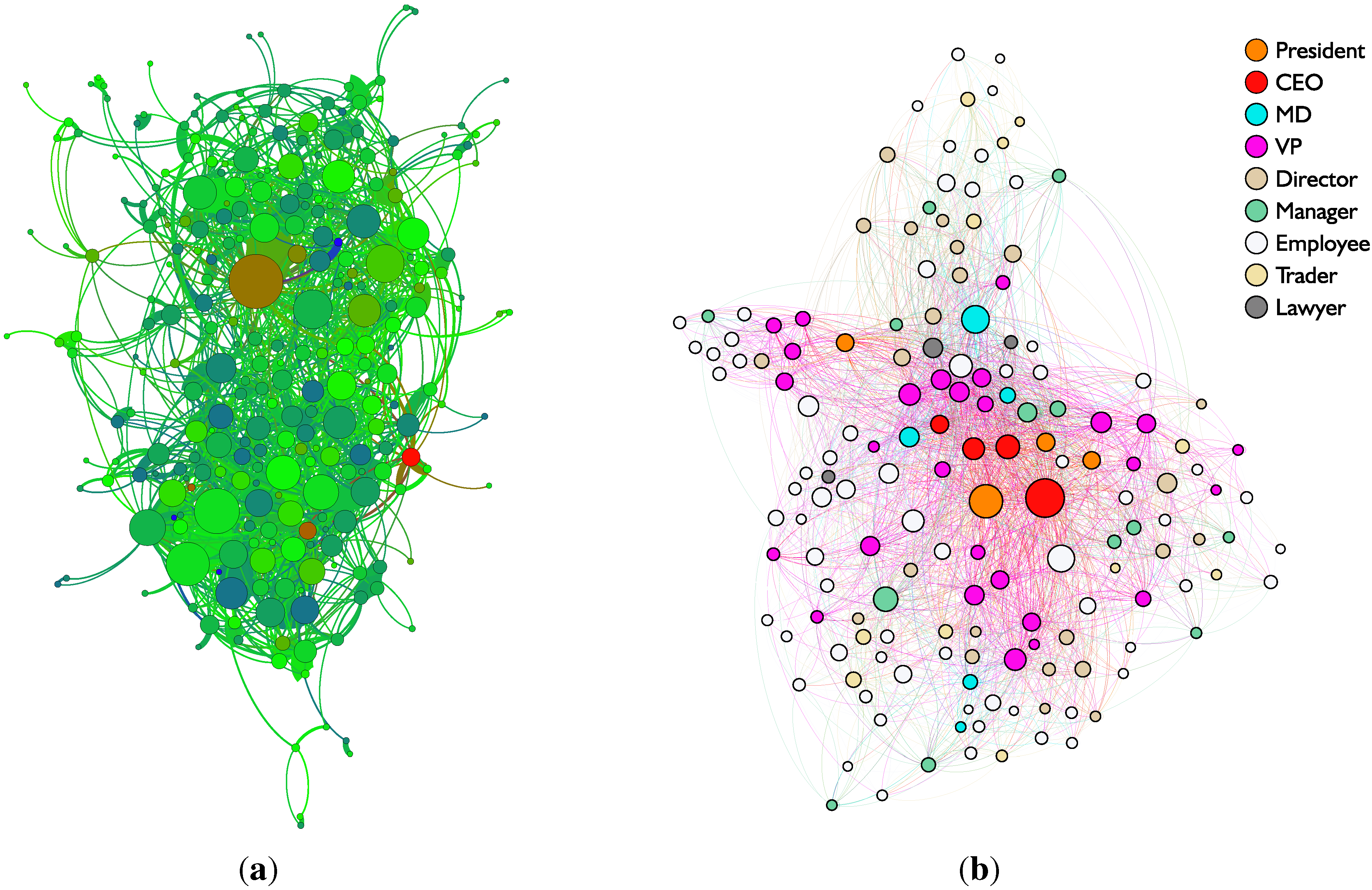
We used two datasets for the experiments. The first is a graph of “who exercises with whom” from a behavioural health study (Figure 2a, $\left|V\right|=279,\left|E\right|=1308$) [29]. Vertices represent participants and are labelled with 28 attributes denoting demographic information and health markers obtained from questionnaire data. Participants were tracked during periods of physical activity; when two people frequently register at the same sensor at the same time, an undirected edge is created, weighted with the number of mutual coincidences. Our second dataset is the “who communicates with whom” graph of the Enron e-mail corpus (Figure 2b, $\left|V\right|=159,\left|E\right|=2667$) [11]. Vertices are labelled with the job role of the employee. Edges are weighted with the number of e-mails exchanged between sender and recipient. As e-mail communications are not symmetric, edges in the Enron graph are directed. Both graphs exhibit a core-periphery structure which is typical of many real-world networks [7].

Figure 2. Input Graph Datasets, from (a) a health study and (b) the Enron e-mail corpus. (a) Undirected graph of who exercised with whom; (b) Directed graph of who e-mailed whom.

Figure 2. Input Graph Datasets, from (a) a health study and (b) the Enron e-mail corpus. (a) Undirected graph of who exercised with whom; (b) Directed graph of who e-mailed whom.

We evaluated Agwan against the following models:

Erdős-Rényi random graph (ER): The ER model $G(n,p)$ has two parameters. We set the number of vertices n and the edge probability p to match the input graphs as closely as possible. We do not expect a very close fit, but the ER model provides a useful baseline.

MAG model with real attributes (MAG-R1) The MAG model with a single real attribute has a set of binary edge probabilities, $\Theta =\left\{p^{ij}\right\}$ instead of a set of BMMs $\Theta =\left\{{\Omega }^{ij}\right\}$.

MAG model with latent attributes (MAG-L$\mathit{x}$): The MAG model also allows for modelling the graph structure using latent attributes. The discrete labels provided in the input graph are ignored; instead MagFit [14] learns the values of a set of latent attributes to describe the graph structure. We vary the number of synthetic attributes x to investigate the relative contributions of vertex labels and edge weights to graph structure.

Agwan model with truncated GMMs: We compare our BMM model to an alternative approach using GMMs [20]. One drawback of using GMMs is that it is possible to draw edge weights $w_{uv}<0$. To avoid negative edge weights, we implement a tabula rasa rule during graph generation, drawing new values from ${\Omega }^{ij}$ until $w_{uv}\ge 0$.

To evaluate the closeness of fit of each model, we use the following statistics:

Vertex Strength: For an unweighted graph, one of the most important measures is the degree distribution (the number of in-edges and out-edges of each vertex). Real-world graphs tend to have heavy-tailed power-law or log-normal degree distributions [2,5]. For a weighted graph, we generalise the concept of vertex degree to vertex strength [30]:

$$\begin{array}{c}\hfill s_u=\sum _{v\ne u}{w}_{uv}\end{array}$$

(12)

We compare using the Complementary Cumulative Distribution Function (CCDF) of the strength of each vertex (both in-strength and out-strength in the case of the directed graph). For Cumulative Distribution Function (CDF) $F\left(x\right)=P(X\le x)$, the CCDF is defined as $\overline{F}=P(X>x)=1-F\left(x\right)$. We show the unnormalised CCDFs in our plots; the normalised value can be obtained by integrating the area under the curve to 1. The CCDF of a power-law function will appear linear when plotted on a log-log scale, while the CCDF of a log-normal function will appear parabolic.

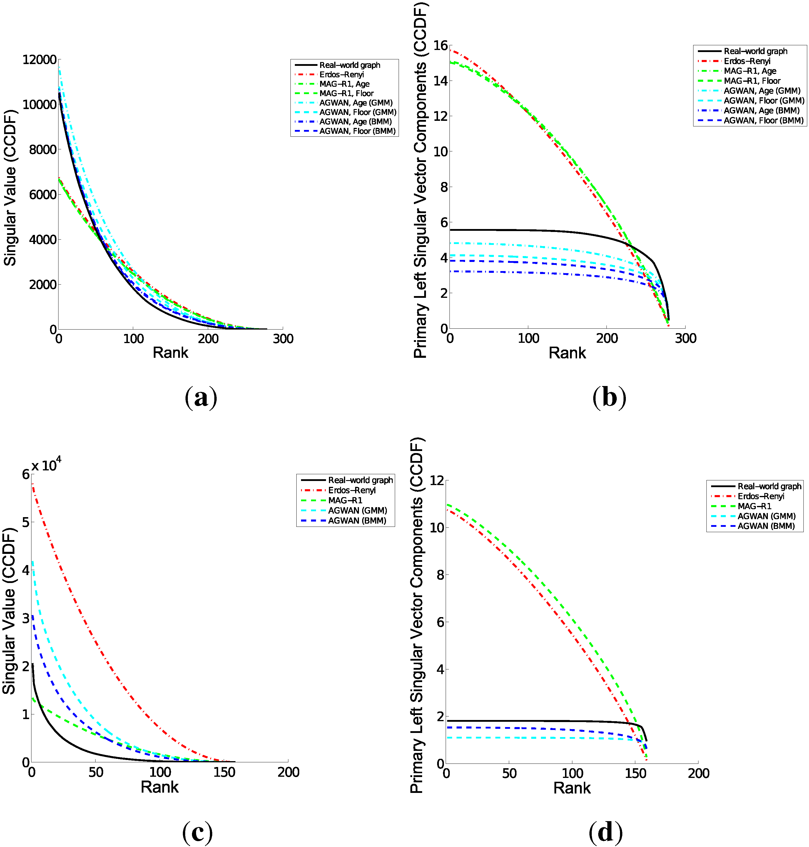
Spectral Properties: We use Singular Value Decomposition (SVD) to calculate the singular values and singular vectors of the graph’s adjacency matrix, which act as a signature of the graph structure. In an unweighted graph, the adjacency matrix contains binary values, for “edge” or “no edge”. In a weighted graph, the adjacency matrix contains the edge weights (with 0 indicating no edge). For SVD $U\Sigma V$, we plot the CCDFs of the singular values Σ and the components of the left singular vector U corresponding to the highest singular value.

Clustering Coefficients: the clustering coefficient C is an important measure of community structure. It measures the density of triangles in the graph, or the probability that two neighbours of a vertex are themselves neighbours [5]. We extend the notion of clustering coefficients to weighted, directed graphs by defining $C_u$, the weighted clustering coefficient for vertex u [30]:

$$\begin{array}{c}\hfill C_u=\frac{{[{\mathsf{W}}_u^{\left[\frac{1}{3}\right]}+{\left({\mathsf{W}}_u^T\right)}^{\left[\frac{1}{3}\right]}]}_{uu}^3}{2[d_u^{tot}(d_u^{tot}-1)-2d_u^{\leftrightarrow }]}\end{array}$$

(13)

where ${\mathsf{W}}_u$ is the weighted adjacency matrix for u and its neighbours, ${\mathsf{W}}^T$ is the transpose of $\mathsf{W}$, $d_u^{tot}$ is the total degree of a vertex (the sum of its in- and out-degrees) and $d_u^{\leftrightarrow }$ is the number of bilateral edges in u (the number of neighbours of u which have both an in-edge and an out-edge between themselves and u). The notation ${\mathsf{A}}_{uu}$ means the u^th element of the main diagonal of $\mathsf{A}$.

Figure 3. Triad Patterns in a Directed Graph. (a) Cycle; (b) Middleman; (c) In; (d) Out.

Figure 3. Triad Patterns in a Directed Graph. (a) Cycle; (b) Middleman; (c) In; (d) Out.

Triad Participation: Closely related to the clustering coefficient is the concept of triangle or triad participation. The number of triangles that a vertex is connected to is a measure of transitivity [5]. For the directed graphs, the triangles have a different interpretation depending on the edge directions. There are four types of triangle pattern [30], as shown in Figure 3. To generalise the concept of triad participation to weighted, directed graphs, we consider each of the four triangle types separately, and sum the total strength of the edges in each triad:

$$\begin{array}{c}\hfill t_u^y=\sum _{v,z\in {\mathsf{W}}_u\backslash u}{\mathbb{W}}_{uvz}^y\end{array}$$

(14)

where $y=\{cycle,middleman,in,out\}$ is the triangle type and ${\mathbb{W}}_{uvz}^y$ is calculated as shown in Figure 3 for each triangle type y.

To give a more objective measure of the closeness of fit between the generated graphs and the input graph, we use a Kolmogorov-Smirnov (KS) test and the L2 (Euclidean) distance between the CCDFs for each statistic. Details are in Appendix B.

5. Results and Discussion

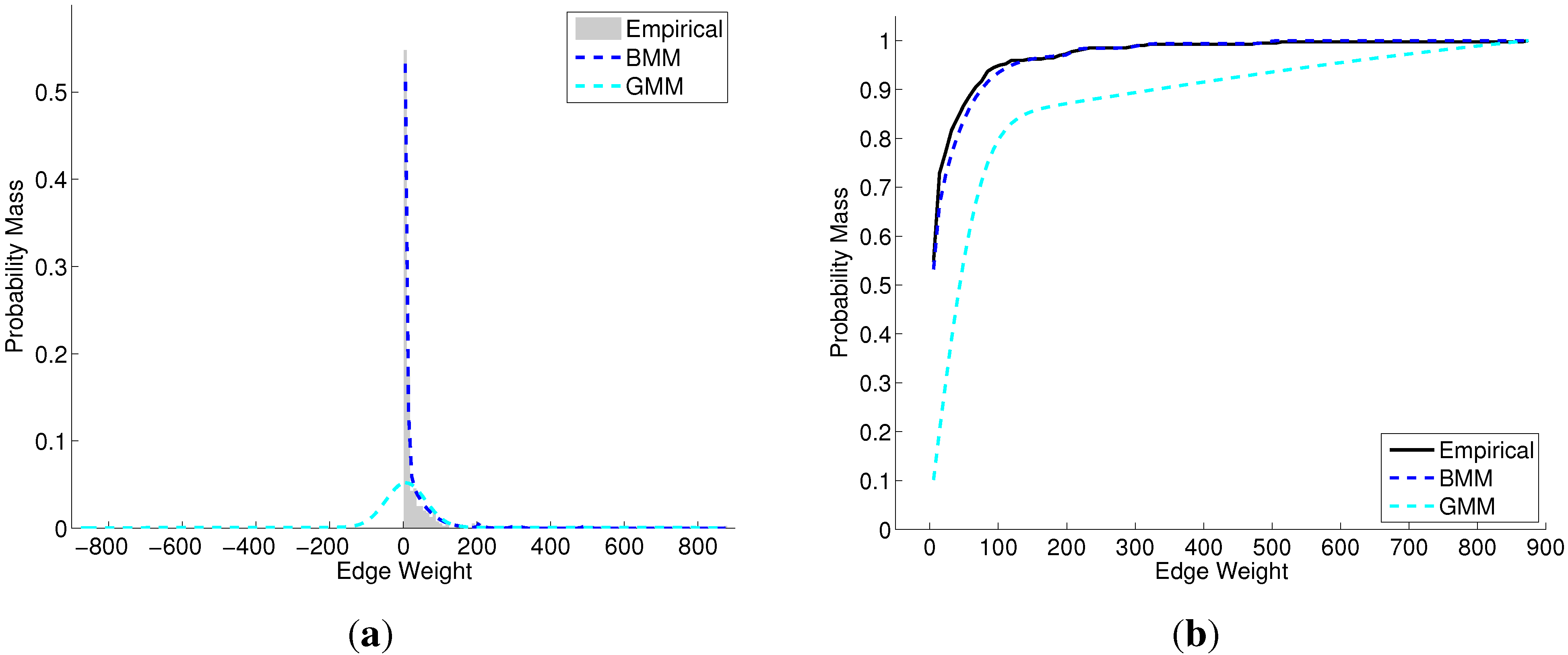
In the experimental data, most of the edge weights follow a heavy-tailed distribution. The BMM achieves a very close fit with its primary mixture component (Figure 4a). The GMM would need several Gaussian components to achieve a similar fit. In practice the VI algorithm for GMMs [18] tries to fit to power law or log-normal distributions using a single Gaussian component, resulting in probability mass being assigned to the area $x<0$, as shown in Figure 4a. This results in a fit that is not as close as the BMM (Figure 4b). To compensate for this effect, we used a truncated GMM for graph generation as discussed in Section 3.2.

Figure 4. Fitting BMM and GMM models to edge weights. (a) Probability Mass Function; (b) Cumulative Distribution Function.

Figure 4. Fitting BMM and GMM models to edge weights. (a) Probability Mass Function; (b) Cumulative Distribution Function.

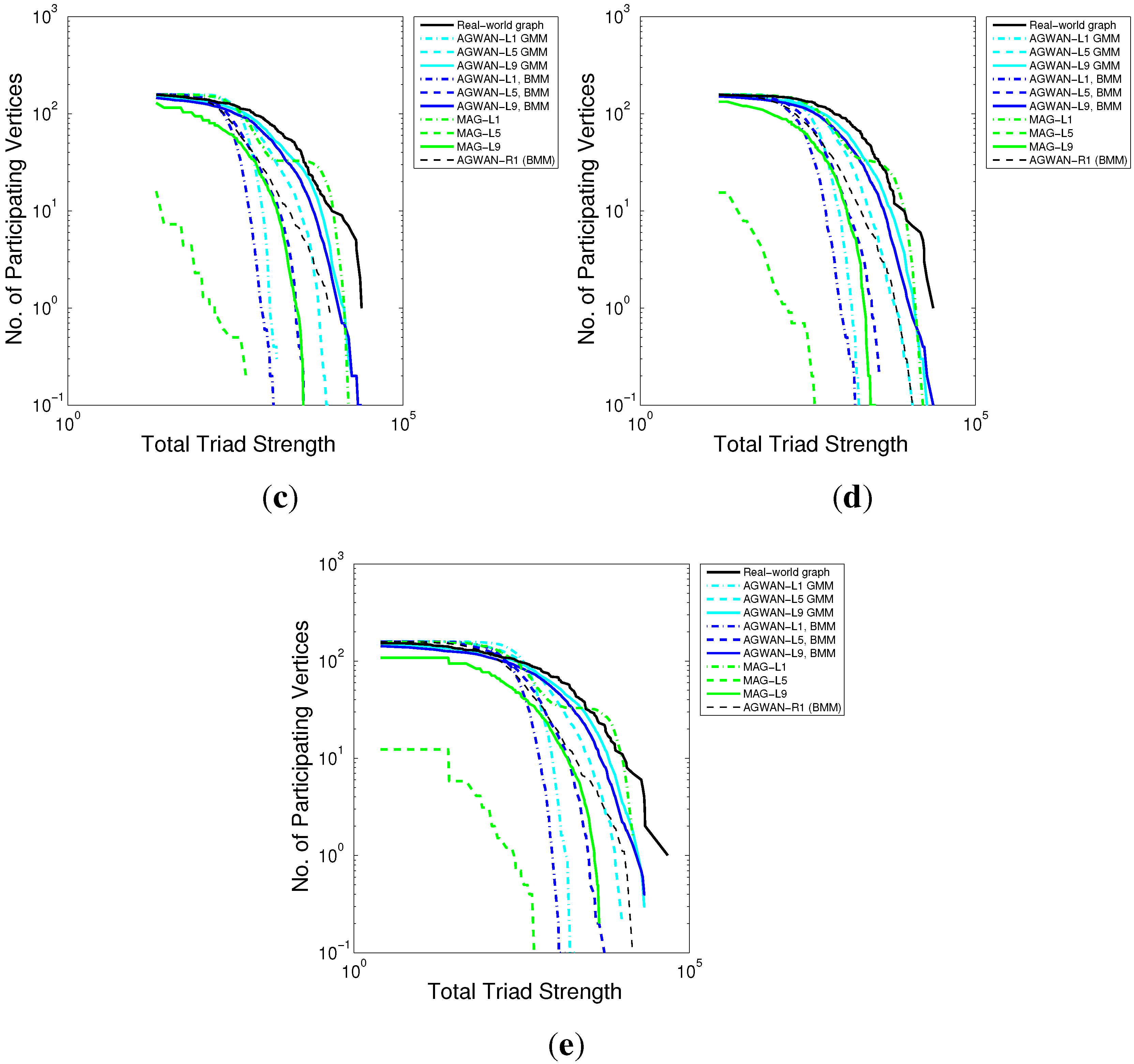
For our experiments, we generated 10 random graphs for each Agwan model. For each graph, we calculated the statistics for vertex strength, spectral properties, clustering and triad participation, as described in the previous section. We calculated the CCDFs for each set of statistics, and averaged the CCDF scores at each x-coordinate value across the 10 graphs, to smooth any random fluctuations. The plots of the averaged CCDFs for each model are shown in Figure 5, Figure 6, Figure 7, Figure 8, Figure 9, Figure 10, Figure 11, Figure 12. Tables for the closeness of fit of each CCDF (KS and L2 statistics) are in Appendix B.

Figure 5. Vertex Strength Distribution—Real Attributes. (a) Undirected; (b) Directed (In-strength); (c) Directed (Out-strength).

Figure 5. Vertex Strength Distribution—Real Attributes. (a) Undirected; (b) Directed (In-strength); (c) Directed (Out-strength).

Figure 6. Spectral Properties—Real Attributes. (a) Undirected—Singular Values; (b) Undirected—Primary Left Singular Vector; (c) Directed—Singular Values; (d) Directed—Primary Left Singular Vector.

Figure 6. Spectral Properties—Real Attributes. (a) Undirected—Singular Values; (b) Undirected—Primary Left Singular Vector; (c) Directed—Singular Values; (d) Directed—Primary Left Singular Vector.

Figure 7. Clustering Coefficients—Real Attributes. (a) Undirected; (b) Directed (In-edges); (c) Directed (Out-edges).

Figure 7. Clustering Coefficients—Real Attributes. (a) Undirected; (b) Directed (In-edges); (c) Directed (Out-edges).

Figure 8. Triad Participation—Real Attributes. (a) Undirected; (b) Directed (Cycles); (c) Directed (Middlemen); (d) Directed (Ins); (e) Directed (Outs).

Figure 8. Triad Participation—Real Attributes. (a) Undirected; (b) Directed (Cycles); (c) Directed (Middlemen); (d) Directed (Ins); (e) Directed (Outs).

Figure 9. Vertex Strength Distribution—Synthetic Attributes. (a) Undirected; (b) Directed (In-strength); (c) Directed (Out-strength).

Figure 9. Vertex Strength Distribution—Synthetic Attributes. (a) Undirected; (b) Directed (In-strength); (c) Directed (Out-strength).

Figure 10. Spectral Properties—Synthetic Attributes. (a) Undirected—Singular Values; (b) Undirected—Primary Left Singular Vector; (c) Directed—Singular Values; (d) Directed—Primary Left Singular Vector.

Figure 10. Spectral Properties—Synthetic Attributes. (a) Undirected—Singular Values; (b) Undirected—Primary Left Singular Vector; (c) Directed—Singular Values; (d) Directed—Primary Left Singular Vector.

Figure 11. Clustering Coefficients—Synthetic Attributes. (a) Undirected; (b) Directed (In-edges); (c) Directed (Out-edges).

Figure 11. Clustering Coefficients—Synthetic Attributes. (a) Undirected; (b) Directed (In-edges); (c) Directed (Out-edges).

Figure 12. Triad Participation—Synthetic Attributes. (a) Undirected; (b) Directed (Cycles); (c) Directed (Middlemen); (d) Directed (Ins); (e) Directed (Outs).

Figure 12. Triad Participation—Synthetic Attributes. (a) Undirected; (b) Directed (Cycles); (c) Directed (Middlemen); (d) Directed (Ins); (e) Directed (Outs).

5.1. Real Attributes

For the undirected graph (Health Study), we show results for two vertex attributes: Age and Floor (the building and floor number where the person works; people who work on the same floor were highly likely to exercise together). For the directed graph (Enron), there is one vertex attribute, the person’s job role.

Vertex Strength (Figure 5): The graphs generated from Agwan have vertex strength distributions which map very closely to the input graphs. The graphs generated from MAG-R1 are better than random (ER), but the vertex strength distribution is compressed into the middle part of the range, with too few high- and low-strength vertices. This indicates that vertex strength depends on both the label distribution and the edge weight distribution; Agwan models both of these effectively.

Spectral Properties (Figure 6): The spectral properties of the Agwan graphs map very closely to the input graphs. The singular values follow the same curve as the input graphs. This is significant as it indicates that graphs generated with Agwan have similar connectivity to the input graph: the primary singular value has been shown to be the most significant measure of graph connectivity [2]. In contrast, MAG-R1 does not preserve the singular value curve, showing a linear relationship instead. MAG-R1 cannot model the singular vector components at all without taking the edge weights into account. These results show that the spectral properties of the graph are dependent on both the vertex label distribution and the edge weight distribution.

Clustering Coefficients (Figure 7): The accuracy of Agwan and MAG-R1 is similar. For the undirected graph, performance is little better than random. For the directed graph, Agwan gives reasonable performance for the low-degree vertices but drops away for the high-degree vertices. In all cases, the clustering is independent of the edge weight distribution. The accuracy of the results depends on which vertex attribute was chosen, implying that some attributes can predict community formation better than others. We hypothesise that cluster formation may in fact be (conditionally) independent of the vertex label values and may be better explained by triadic closure [5]: links are likely to form between two people who share a mutual friend, independently from their vertex attributes. The apparent dependency on vertex labels may be an artefact of the connection to the mutual friend, rather than the true explanation of why clustering asises. This aspect of network formation requires further investigation.

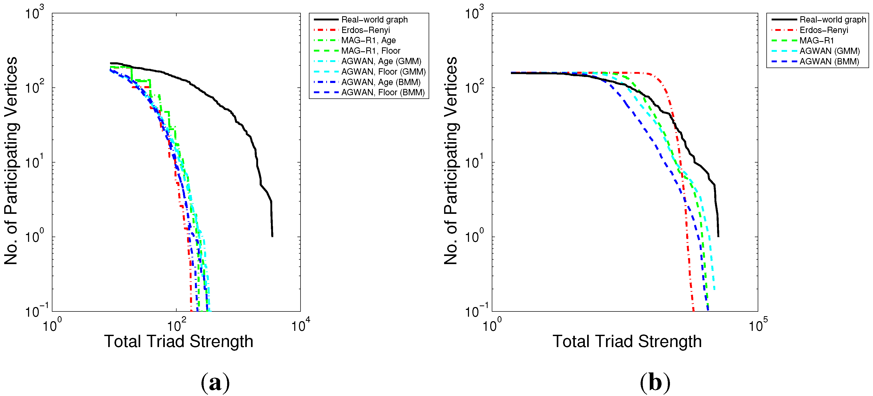
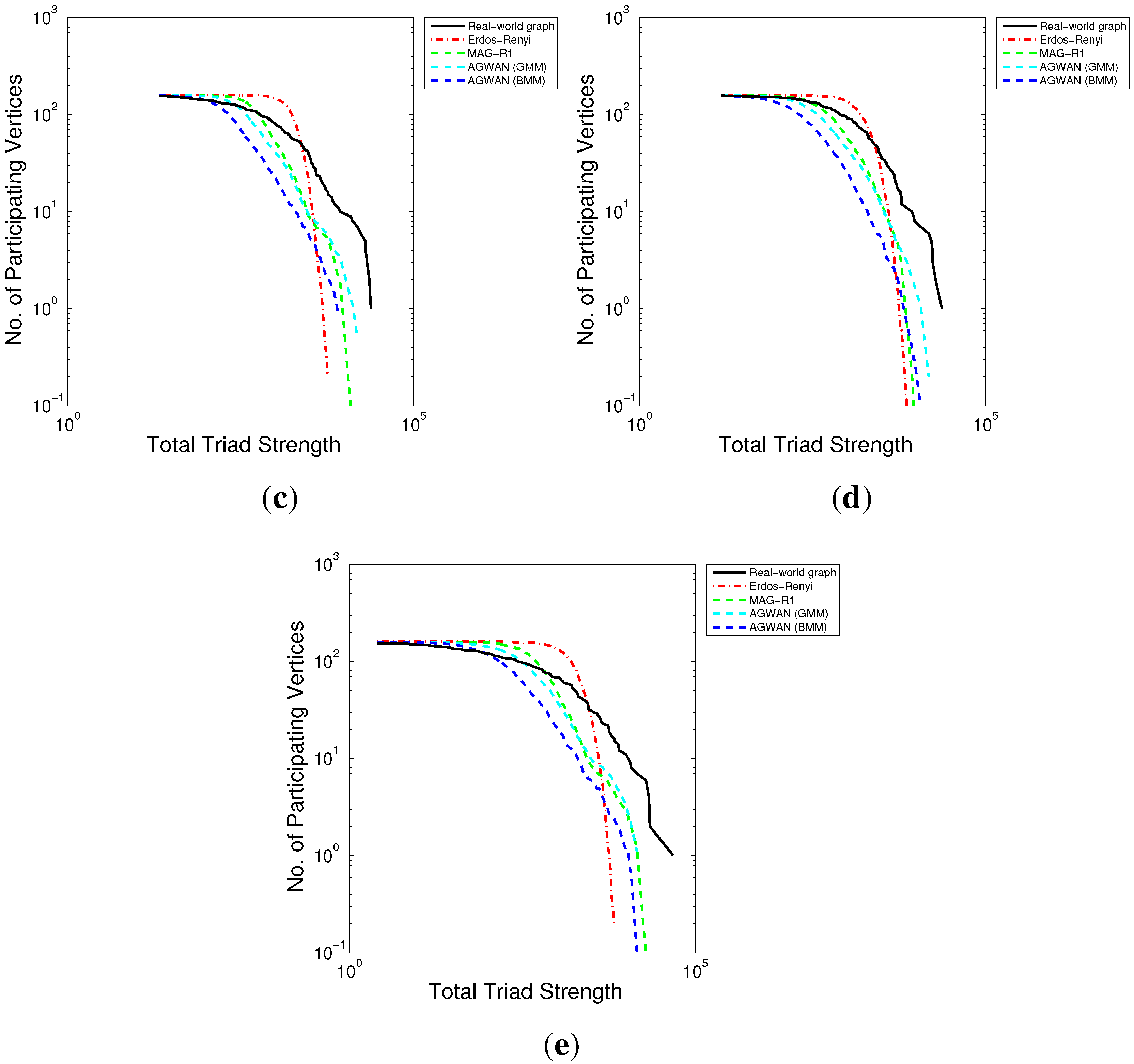
Triad Participation (Figure 8): Similar to clustering, triad participation appears to be dependent to some extent on vertex label values but independent of the edge weight distribution. We hypothesise that like clustering, the apparent dependency between vertex label and triad participation values may be due to triadic closure, which is not currently modelled by either MAG or Agwan.

5.2. Synthetic Attributes

The second set of experiments ignore the real attributes of the graph, replacing them with a set of randomly generated synthetic attributes. The purpose is to evaluate the relative contribution of the discrete vertex labels and numeric attributes to the graph structure. By reducing the number of numeric attributes to zero, we can evaluate the contribution of the numeric attributes in isolation.

We replaced the real labels in the input graph with a synthetic vertex attribute taking $2^0\dots 2^9$ values allocated uniformly at random, then learned the edge weight distributions using VI as normal. We compare our results with an alternate interpretation of the MAG model, which ignores the true attribute values from the input graph and represents attributes as latent variables, which are learned using a VI EM approach [14]. We also show Agwan with one real attribute for comparison.

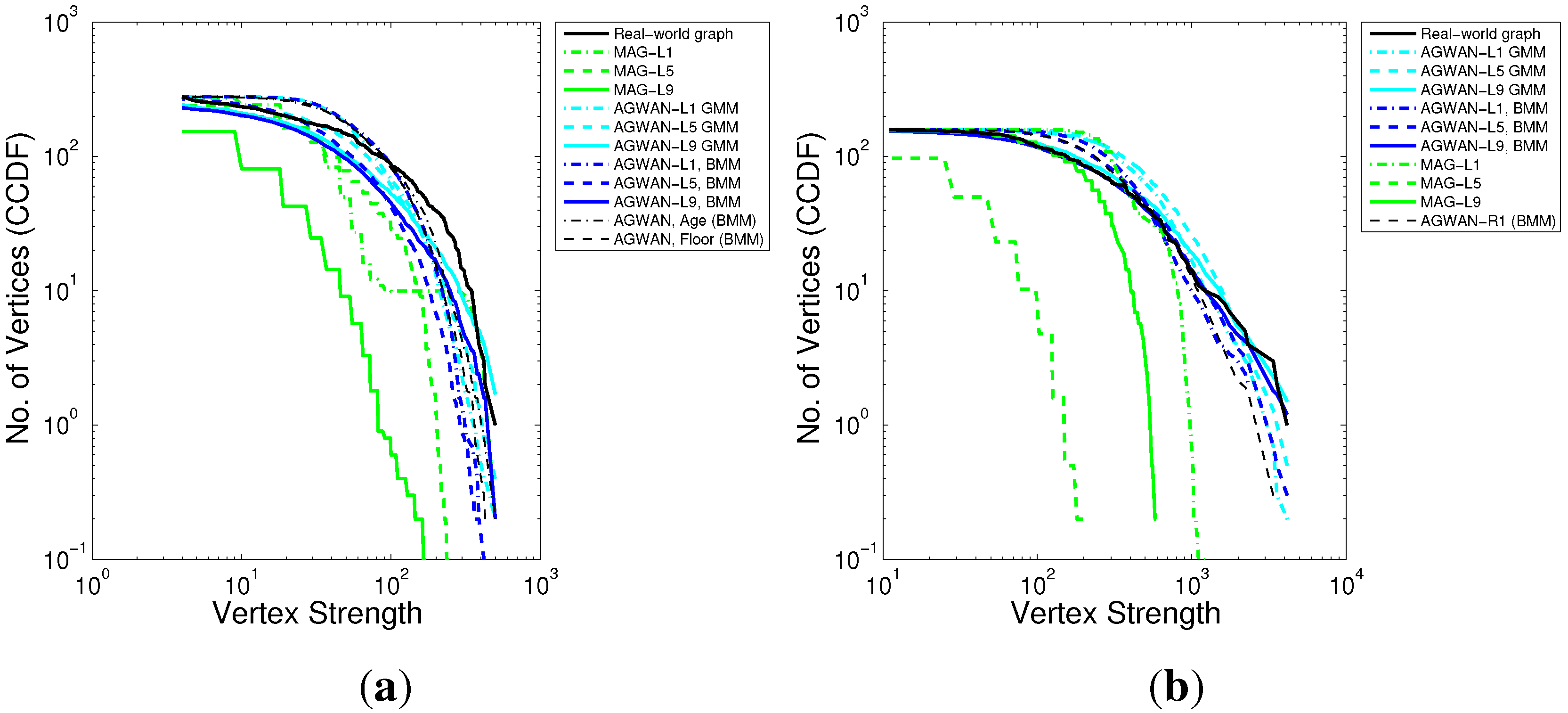
Vertex Strength (Figure 9): Agwan with synthetic attributes significantly outperforms MAG for the accuracy of the vertex strength distribution, and has similar accuracy to Agwan-R1. Varying the number of synthetic attributes has a small effect on the accuracy. We conclude that vertex strength is dependent on both edge weight and vertex label distribution, but the edge weights play a more important role.

Spectral Properties (Figure 10): Agwan has a very close fit to the spectral properties of the input graphs. Varying the number of attributes has a moderate effect on the closeness of fit. On the undirected graph, MAG-L9 matches the singular vector very closely but performs poorly with the singular values; in general, MAG is a poor fit as the edge weight distribution is not taken into account. These results confirm that the spectral properties are dependent on both the vertex label distribution and the edge weight distribution, and the degrees of freedom of the vertex labels are important.

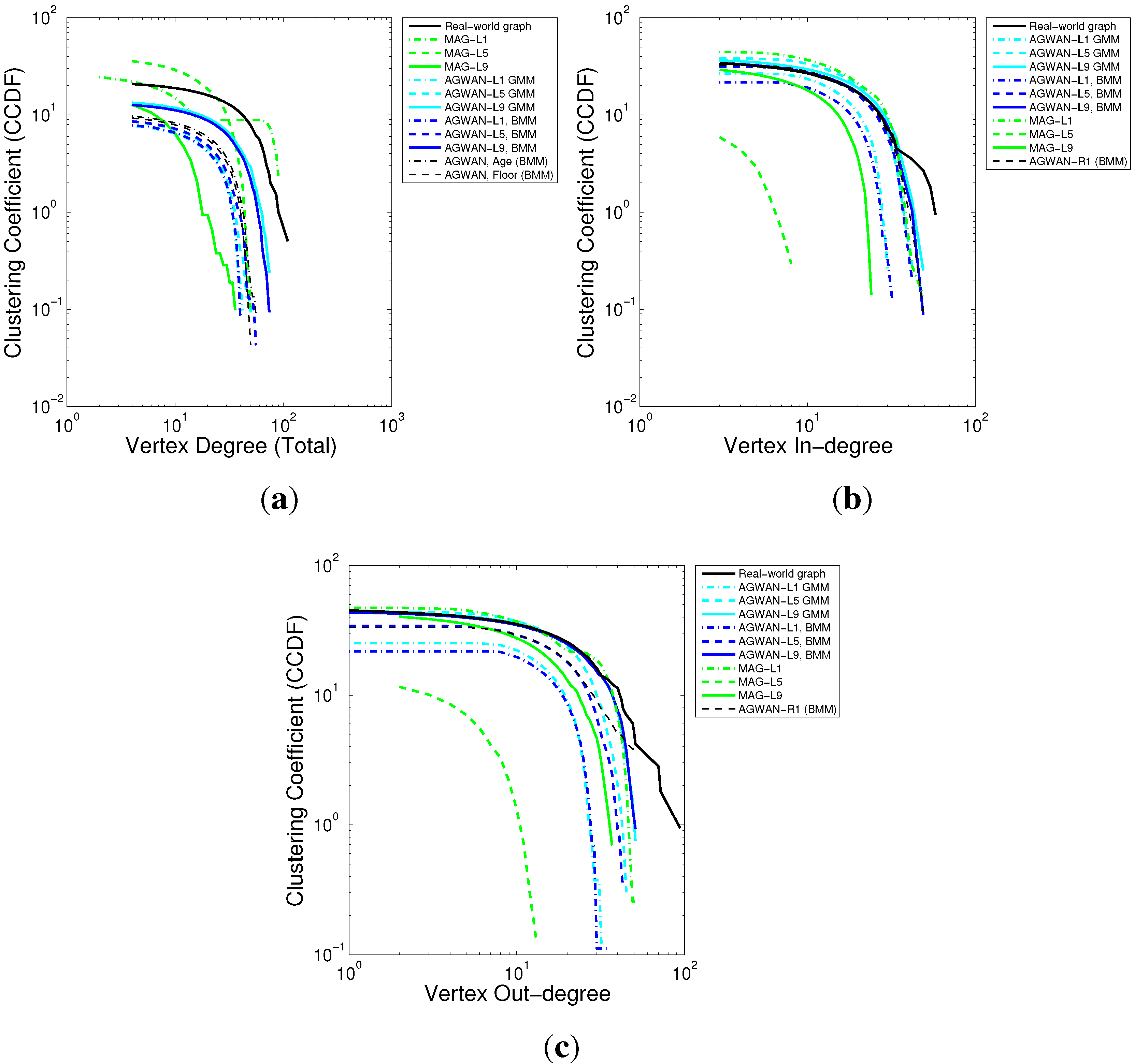
Clustering Coefficients (Figure 11): Agwan and MAG are both significantly more accurate using synthetic attributes than with real attributes. This (somewhat surprising) result implies that clustering is not closely related to the real attribute values. While real labels appear to be influenced by the (unobserved) process which gives rise to clustering, synthetic labels with more degrees of freedom can model it more accurately. We note that Agwan performs better where there are more degrees of freedom, while MAG performs better with few degrees of freedom (due to the independence assumption mentioned in Section 3.3). As before, clustering appears to be independent of the edge weight distribution.

Triad Participation (Figure 12): Similarly to clustering, Agwan and MAG are both more accurate using synthetic attributes than they were with real attributes. The effects of degrees of freedom of the synthetic attributes is even more pronounced than it was for clustering: Agwan-L9 has a good fit whereas Agwan-L1 is not so good. Edge weights appear to have little influence.

5.3. Graph Evolution

One of the goals of our model is to generate synthetic graphs which are larger than the input graph. We conducted experiments to measure how Agwan graph properties change as the number of vertices is increased. We generated sets of random graphs from the same model, with increasing numbers of vertices $N=\{10,20,\dots ,100,[1]200,\dots ,3000\}$ vertices and measured the size of the giant component, the density and the diameter.

Giant Component: We measured the proportion of vertices in the largest component of the graph as the graph grows in size. Figure 13 shows that a giant component forms quickly, as in real graphs [5].

Figure 13. Giant Component. (a) Undirected; (b) Directed.

Figure 13. Giant Component. (a) Undirected; (b) Directed.

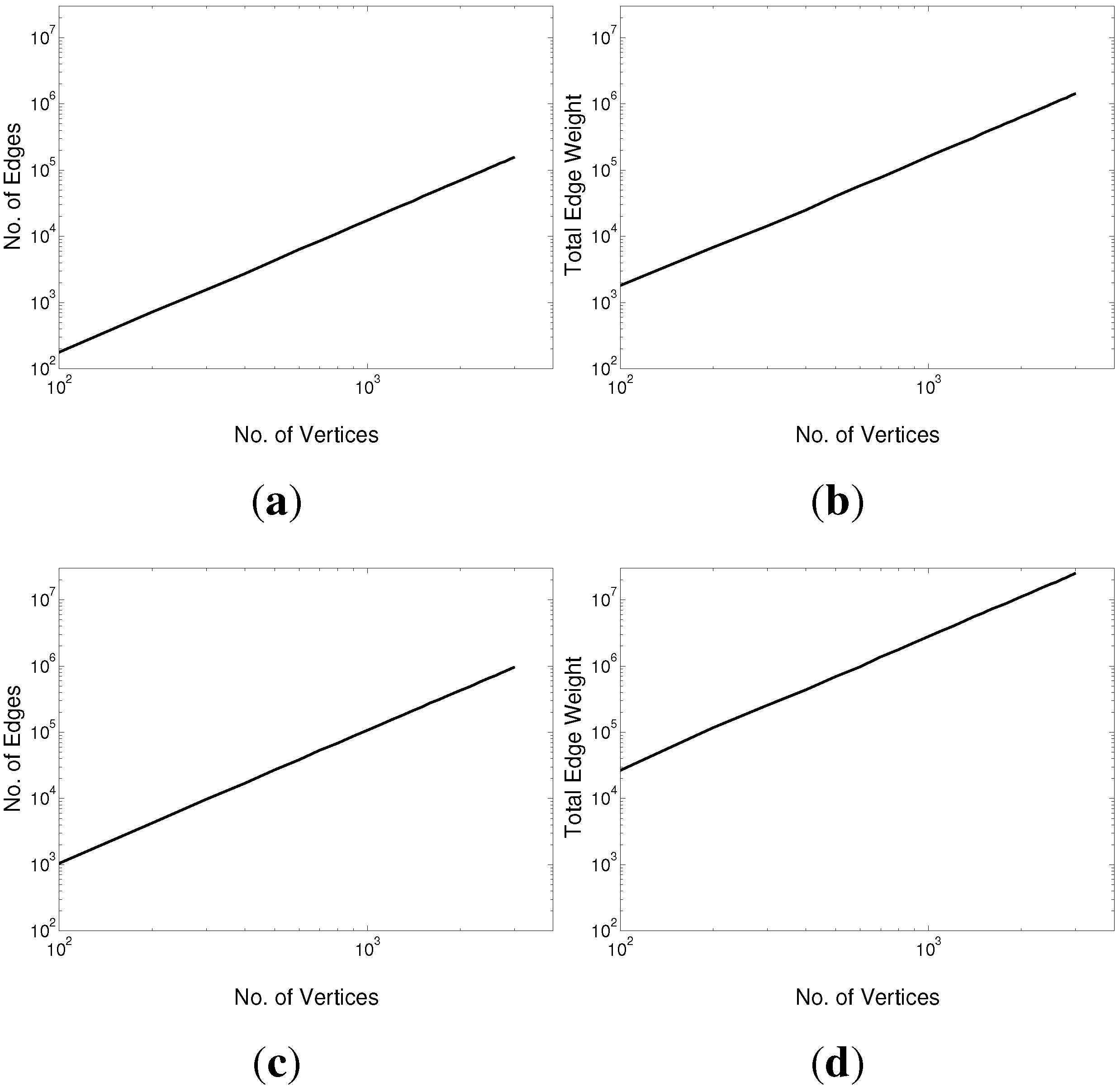
Densification Power Law: We measured graph densification as the ratio of the number of vertices to the number of edges as the graph grows in size. Figure 14 shows that Agwan graphs densify as they grow, as in real graphs. Real-world graphs have $e\left(t\right)\propto v{\left(t\right)}^{\gamma }$, with power-log exponent γ typically in the range $(1,2)$ [4]. When $\gamma =1$, the rate of edge growth is linear in the number of vertices; $\gamma =2$ means that on average, each vertex has edges to a constant fraction of all vertices. As Figure 14 shows, Agwan graphs have $\gamma \simeq 2$, because the model learns its edge probabilities independently from the size of the input graph. This means that Agwan overestimates density when generating graphs larger than the input graph.

Figure 14. Densification Power Law. (a) Undirected, unweighted; (b) Undirected, weighted; (c) Directed, unweighted; (d) Directed, weighted.

Figure 14. Densification Power Law. (a) Undirected, unweighted; (b) Undirected, weighted; (c) Directed, unweighted; (d) Directed, weighted.

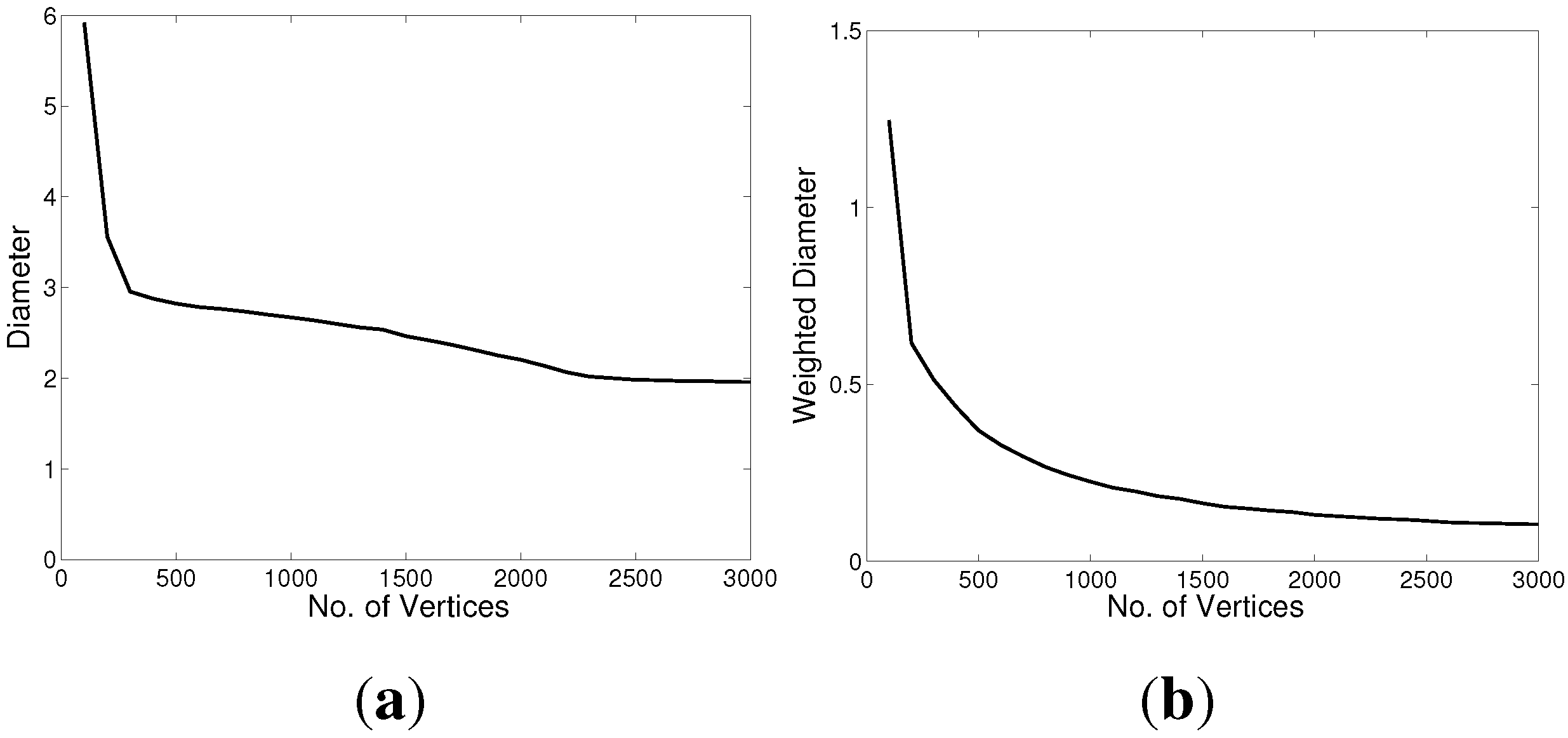
Shrinking Diameter Effect (Figure 15): Agwan graphs exhibit the Small World Effect [5] and the unweighted diameter shrinks as the graphs grow, as in real graphs [4]. As the weighted diameter was calculated using Johnson’s algorithm [31], which treats the edge weight as a cost function, we used the reciprocal of the edge weights. With this interpretation, the weighted diameter also shrinks as the graphs grow. It is interesting to note that the weighted diameters decay following a power law (with exponent $\gamma =-0.72$ for the undirected graph and $\gamma =-0.65$ for the directed graph).

Figure 15. Shrinking Diameter Effect. (a) Undirected, unweighted; (b) Undirected, weighted; (c) Directed, unweighted; (d) Directed, weighted.

Figure 15. Shrinking Diameter Effect. (a) Undirected, unweighted; (b) Undirected, weighted; (c) Directed, unweighted; (d) Directed, weighted.

6. Conclusions and Future Work

In this paper, we presented Agwan, a generative model for random graphs with discrete labels and weighted edges. We included a fitting algorithm to learn a model of edge weights from real-world graphs, and an algorithm to generate random labelled, weighted graphs with similar characteristics to the input graph.

We measured the closeness of fit of our generated graphs to the input graph over a range of graph statistics, and compared our approach to the state-of-the-art in random graph generative algorithms. Our results and findings are summarised in Table 1.

Table 1. Summary of results and findings: dependencies between graph labels and weights and structural properties (${}^{*}$hypothesised); relative accuracy of the properties of weighted graphs generated using Agwan and MAG models.

Statistic	Vertex Labels	Edge Weights	Agwan	MAG
Vertex Strength	Dependent	Dependent	Accurate	Less accurate
Singular Values	Dependent	Dependent	Accurate	Less accurate
Primary Singular Vector	Partially	Dependent	Accurate	Poor
	Dependent
Clustering Coefficients	Conditionally	Independent	Less accurate when using real attributes
	Independent${}^{*}$		More accurate with synthetic attributes
Triad Participation	Conditionally	Independent	Less accurate when using real attributes
	Independent${}^{*}$		More accurate with synthetic attributes

Table 1. Summary of results and findings: dependencies between graph labels and weights and structural properties (${}^{*}$hypothesised); relative accuracy of the properties of weighted graphs generated using Agwan and MAG models.

Statistic	Vertex Labels	Edge Weights	Agwan	MAG
Vertex Strength	Dependent	Dependent	Accurate	Less accurate
Singular Values	Dependent	Dependent	Accurate	Less accurate
Primary Singular Vector	Partially	Dependent	Accurate	Poor
	Dependent
Clustering Coefficients	Conditionally	Independent	Less accurate when using real attributes
	Independent${}^{*}$		More accurate with synthetic attributes
Triad Participation	Conditionally	Independent	Less accurate when using real attributes
	Independent${}^{*}$		More accurate with synthetic attributes

Our results demonstrate that Agwan produces an accurate model of the weighted input graphs. The Agwan graphs reproduce many of the properties of the input graphs, including formation of a giant component, heavy-tailed degree distribution, Small World property, Densification Power Law and shrinking diameter effect. Vertex strength and spectral properties were modelled very closely, indicating that these properties are indeed dependent on vertex labels and edge weights. For clustering and triad participation, it appears that these properties are independent of the edge weight distribution. While there appears to be a relationship with the vertex label distribution, we suggest that this may be an artefact of the true process giving rise to these properties, triadic closure. Further research is required into the relationship between vertex attributes and triangle formation in graphs.

We investigated the accuracy of modelling edge weights using BMMs and compared to a previous approach which used GMMs. The edge weights often follow a power-law distribution, which the BMM approach fits more closely, particularly in the lower range of edge weight values. In general, BMMs are more suitable for bounded data; probability mass can only be assigned to the valid range of weight values. For the GMM model, we compensated for this by truncating the GMM during graph generation. We expected that Agwan (BMM) would consistently outperform Agwan (GMM), but the truncated GMM performed surprisingly well. We propose to conduct experiments on a wider range of datasets to investigate this further. It would also be interesting to compare with Poisson Mixture Models to model discrete edge weights.