On the Accessibility of Newton’s Method under a Hölder Condition on the First Derivative

Abstract

We see how we can improve the accessibility of Newton’s method for approximating a solution of a nonlinear equation in Banach spaces when a center Hölder condition on the first derivative is used to prove its semi-local convergence.

1. Introduction

It is often necessary in many scientific and engineering problems to find a root of a nonlinear equation. To solve this equation, we can use iterative methods. To give sufficient generality to the problem of approximating a solution of a nonlinear equation by iterative methods, we are concerned, in this work, with the problem of approximating a locally-unique solution $x^{*}$ of the equation $F\left(x\right)=0$, where F is a nonlinear operator defined on a nonempty open convex subset Ω of a Banach space X with values in a Banach space Y, so that many scientific and engineering problems can be written as a nonlinear equation in Banach spaces.

Newton’s method is probably the best-known iterative method, and it is well known that it converges quadratically. Newton’s method for solving scalar equations was extended to nonlinear equations in Banach spaces by Kantorovich in 1948 [1] in the following way:

$$x_0\text{given}\text{in}\Omega ,x_n=x_{n-1}-{\left[F^{\prime }\left(x_{n-1}\right)\right]}^{-1}F\left(x_{n-1}\right),n\in \mathbb{N},$$

(1)

where $F^{\prime }$ is the Fréchet derivative of the operator F. For this reason, many authors refer to it as the Newton–Kantorovich method.

Kantorovich proved the semi-local convergence of Newton’s method under the hypothesis that the operator involved F is twice differentiable Fréchet with bounded second derivative:

There exists a constant $C\ge 0$, such that $\parallel F^{\prime \prime }\left(x\right)\parallel \le C$ for $x\in \Omega$.

It is well known that this condition can be replaced by a Lipschitz condition on the first derivative $F^{\prime }$ of the operator involved [2]:

There exists a constant $L\ge 0$, such that $\parallel F^{\prime }\left(x\right)-F^{\prime }\left(y\right)\parallel \le L\parallel x-y\parallel$ for $x,y\in \Omega$.

In view of the applications, numerous papers have recently appeared where the convergence of the method is proven under different conditions for the derivatives of the operator F. A known variant is the study of the convergence of the method under a Hölder condition on the first derivative [3,4,5]:

There exist two constants $K\ge 0$ and $p\in (0,1]$ such that $\parallel F^{\prime }\left(x\right)-F^{\prime }{\left(y\right)\parallel \le K\parallel x-y\parallel }^p$ for $x,y\in \Omega$.

In order to improve the accessibility of Newton’s method under the last condition, we can use different strategies that change the condition. In this work, we use a similar one as that used by Argyros in [6] for the Lipschitz condition on the first derivative $F^{\prime }$, which consists of noticing that, as a consequence of the last condition being satisfied in Ω, we have, for the starting point $x_0$, that:

• There exist two constants $K_0\ge 0$ and $p\in (0,1]$, such that $\parallel F^{\prime }\left(x\right)-F^{\prime }\left(x_0\right)\parallel \le K_0{\parallel x-x_0\parallel }^p$ for $x\in \Omega$,

with $K_0\le K$. We then say that $F^{\prime }$ is center Hölder in $x_0$.

In this paper, we focus our attention on the analysis of the semi-local convergence of Sequence (1), which is based on demanding the last condition to the initial approximation $x_0$ and provides the so-called domain of parameters corresponding to the conditions required for the initial approximation that guarantee the convergence of Sequence (1) to the solution $x^{*}$.

In this work, we carry out an analysis of the domain of parameters for Newton’s method under the last two conditions for $F^{\prime }$ and use a technique based on recurrence relations. As a consequence, we improve the domains of parameters associated with the semi-local convergence result given for Newton’s method by Hérnández in [4].

We prove in this paper that center conditions on the first derivative of the operator involved in the solution of nonlinear equations play an important role in the semi-local convergence of Newton’s method, since we can improve the accessibility of Newton’s method from them.

Throughout the paper, we denote $\overline{B(x,\varrho )}=\{y\in X;\parallel y-x\parallel \le \varrho \}$ and $B(x,\varrho )=\{y\in X;\parallel y-x\parallel <\varrho \}$.

2. Preliminaries

The best-known semi-local convergence result for Newton’s method under a Hölder condition on the first derivative of the operator involved, when the technique of recurrence relations is used to prove it, is that given by Hernández in [4], which is established under the following conditions:

(A1)

There exists ${\Gamma }_0={\left[F^{\prime }\left(x_0\right)\right]}^{-1}\in \mathcal{L}(Y,X)$, for some $x_0\in \Omega$, with $\parallel {\Gamma }_0\parallel \le \beta$ and $\parallel {\Gamma }_{0}F\left(x_0\right)\parallel \le \eta$, where $\mathcal{L}(Y,X)$ is the set of bounded linear operators from Y to X.

(A2)

There exist two constants $K\ge 0$ and $p\in (0,1]$, such that $\parallel F^{\prime }\left(x\right)-F^{\prime }{\left(y\right)\parallel \le K\parallel x-y\parallel }^p$ for $x,y\in \Omega$.

(A3)

If $\xi \left(p\right)$ is the unique zero of the auxiliary function:

$$\varphi (x;p)={(1+p)}^p{(1-x)}^{1+p}-x^p,p\in (0,1],$$

(2)

in the interval $\left(0,\frac{1}{2}\right]$, it is satisfied that $h=K\beta {\eta }^p\le \xi \left(p\right)$ and $B(x_0,R)\subset \Omega$, where $R=\frac{(1+p)(1-h)}{(1+p)-(2+p)h}\eta$.

Theorem 1. (Theorem 2.1 of [4]) Let $F:\Omega \subseteq X⟶Y$ be a continuously-differentiable operator defined on a nonempty open convex domain Ω of a Banach space X with values in a Banach space Y. Suppose that Conditions (A1)(A3) are satisfied. Then, Newton’s sequence, given by (1), converges to a solution $x^{*}$ of the equation $F\left(x\right)=0$, starting at $x_0$, and $x_n,x^{*}\in \overline{B(x_0,R)}$, for all $n=0,1,2,\dots$

Note that Condition (A1), required for the initial approximation $x_0$, defines the parameters β and η, and Condition (A2), required for the operator F, defines the parameter K fixed for all point of Ω. Observe that, every point $z\in \Omega$, such that the operator ${\left[F^{\prime }\left(z\right)\right]}^{-1}$ exists with $\parallel {\left[F^{\prime }\left(z\right)\right]}^{-1}\parallel \le \beta$ and $\parallel {\left[F^{\prime }\left(z\right)\right]}^{-1}F\left(z\right)\parallel \le \eta$, has associated the pair $(K,\beta {\eta }^p)$ of the $xy$-plane, where $x=K$ and $y=\beta {\eta }^p$. In addition, fixed $p\in (0,1]$, if we consider the set:

$${\mathcal{D}}_{\text{T}}=\left\{(x,y)\in {\mathbb{R}}^2:xy\le \xi \left(p\right)\right\},$$

we can observe that every point z, such that its associated pair $(K,\beta {\eta }^p)$ belongs to ${\mathcal{D}}_{\text{T}}$, can be chosen as the starting point for Newton’s method, so that the method converges to a solution $x^{*}$ of the equation $F\left(x\right)=0$ when it starts at z. The set ${\mathcal{D}}_{\text{T}}$ is then called the domain of parameters associated with Theorem 1 and can be drawn by choosing $x=K$, $y=\beta {\eta }^p$ and coloring the region of the $xy$-plane whose points satisfy the condition $h\le \xi \left(p\right)$ (namely, $xy\le \xi \left(p\right)$) of the Theorem 1. 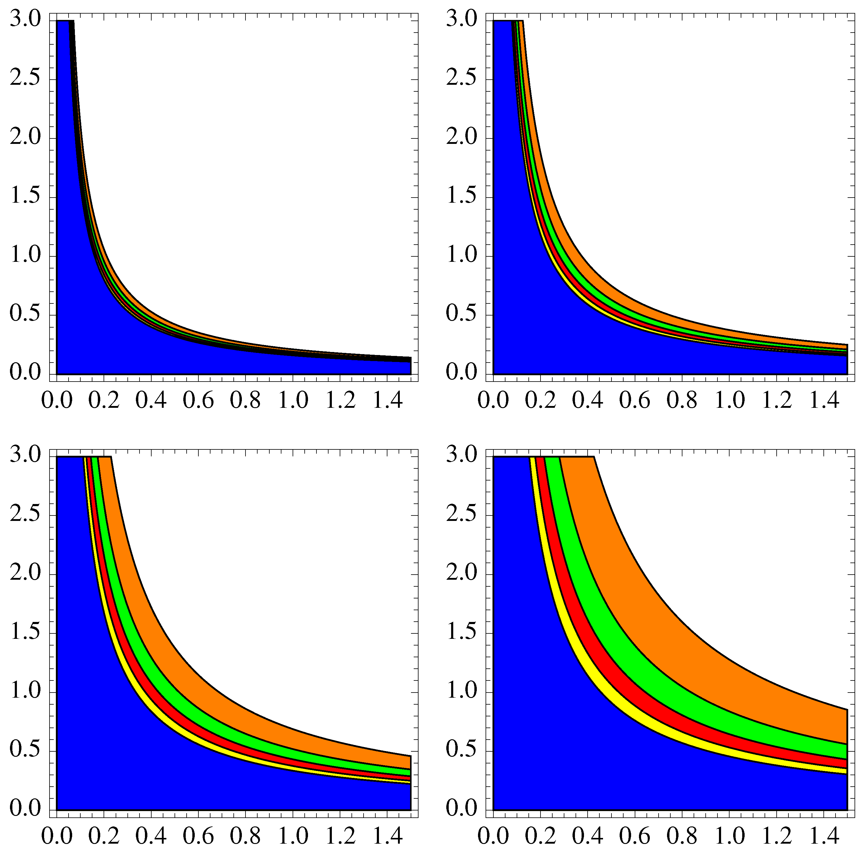In Figure 1, we see the domain of parameters ${\mathcal{D}}_{\text{T}}$ (blue region).

In relation to the above, we can think that the larger the size of the domain of parameters is, the more possibilities we have for choosing good starting points for Newton’s method. As a consequence, we are interested in ${\mathcal{D}}_{\text{T}}$ being as big as possible, since this fact allows us to find a greater number of good starting points for Newton’s method.

3. Semi-Local Convergence of Newton’s Method

To improve the semi-local convergence of Newton’s method from increasing the domain of parameters ${\mathcal{D}}_{\text{T}}$, we consider a procedure that consists of observing that, as a consequence of Condition (A2), once $x_0\in \Omega$ is fixed, the condition:

$$\parallel F^{\prime }\left(x\right)-F^{\prime }\left(x_0\right)\parallel \le K_0{\parallel x-x_0\parallel }^p,x\in \Omega ,$$

(3)

is satisfied with $K_0\le K$. Then, by considering jointly the parameters K and $K_0$, we can relax the semi-local convergence conditions of Newton’s method given in Theorem 1 and obtain a larger domain of parameters.

Now, we present a semi-local convergence result for Newton’s method under Condition (A1) for the starting point $x_0$ and Condition (A2) for the first derivative $F^{\prime }$. Note that Condition (3) follows from Condition (A2) for the starting point $x_0$. In addition, we obtain a semi-local convergence result by combining Conditions (A2) and (3), which allows increasing the domain of parameters ${\mathcal{D}}_{\text{T}}$, so that the possibility of choosing good starting points for Newton’s method is increased, as we can see later in the applications. In particular, we study the convergence of Newton’s method to a solution of the equation $F\left(x\right)=0$ under certain conditions for the pair $(F,x_0)$. From some real parameters, a system of four recurrence relations is constructed in which two sequences of positive real numbers are involved. The convergence of Newton’s method is then guaranteed from them.

3.1. Auxiliary Scalar Sequences

From Conditions (A1)–(A2), we define $\gamma =\epsilon h$, $b_0=h$ and $\delta =\frac{\gamma }{(1+p)(1-\gamma )}$, where $\epsilon =\frac{K_0}{K}\in [0,1]$. Now, we define $b_1=\frac{{\delta }^p}{1-\gamma }{b}_0$ and:

$$\begin{array}{cc}\hfill a_n& =\frac{b_n}{(1+p)(1-b_n)},n\ge 1,\hfill \end{array}$$

(4)

$$\begin{array}{cc}\hfill b_n& =\frac{b_{n-1}{a}_{n-1}^p}{1-b_{n-1}},n\ge 2.\hfill \end{array}$$

(5)

Observe that we consider the case $b_0>0$, since if $b_0=0$, a trivial problem results, as the solution of the equation $F\left(x\right)=0$ is $x_0$.

Next, we prove the following four recurrence relations for Sequences (1), (4) and (5):

$$\begin{array}{cc}\hfill \parallel {\Gamma }_1\parallel & =\parallel {\left[F^{\prime }\left(x_1\right)\right]}^{-1}\parallel \le \frac{\parallel {\Gamma }_0\parallel }{1-\gamma },\hfill \end{array}$$

(6)

$$\begin{array}{cc}\hfill \parallel x_2-x_1\parallel & \le \delta \parallel x_1-x_0\parallel ,\hfill \end{array}$$

(7)

$$\begin{array}{cc}\hfill K\parallel {\Gamma }_1\parallel \parallel x_2-x_1{\parallel }^p& \le b_1,\hfill \end{array}$$

(8)

$$\begin{array}{cc}\hfill \parallel x_2-x_0\parallel & \le (1+\delta )\parallel x_1-x_0\parallel ,\hfill \end{array}$$

(9)

provided that:

$$x_1\in \Omega and\gamma <1.$$

(10)

If $x_1\in \Omega$, then:

$$\parallel I-{\Gamma }_0{F}^{\prime }\left(x_1\right)\parallel \le \parallel {\Gamma }_0\parallel \parallel F^{\prime }\left(x_0\right)-F^{\prime }\left(x_1\right)\parallel \le K\beta {\eta }^p=h<1.$$

Then, by the Banach lemma on invertible operators, it follows that the operator ${\Gamma }_1$ exists and:

$$\parallel {\Gamma }_1\parallel \le \frac{\parallel {\Gamma }_0\parallel }{1-\parallel I-{\Gamma }_0{F}^{\prime }\left(x_1\right)\parallel }\le \frac{\parallel {\Gamma }_0\parallel }{1-\gamma }.$$

After that, from Taylor’s series and Sequence (1), we have:

$$\parallel F\left(x_1\right)\parallel =∥{\int }_0^1(F^{\prime }(x_0+\tau (x_1-x_0))-F^{\prime }\left(x_0\right))(x_1-x_0)d\tau ∥\le \frac{K_0{\eta }^p}{1+p}\parallel x_1-x_0\parallel .$$

Thus,

$$\begin{array}{cc}\hfill \parallel x_2-x_1\parallel & \le \parallel {\Gamma }_1\parallel \parallel F\left(x_1\right)\parallel \le \delta \parallel x_1-x_0\parallel \hfill \\ \hfill \parallel {\Gamma }_1\parallel \parallel x_2-x_1{\parallel }^p& \le \frac{K{\delta }^p}{1-\gamma }\parallel {\Gamma }_0\parallel \parallel x_1-x_0{\parallel }^p\le b_1,\hfill \\ \hfill \parallel x_2-x_0\parallel & \le \parallel x_2-x_1\parallel +\parallel x_1-x_0\parallel \le (1+\delta )\parallel x_1-x_0\parallel <\left(1+\frac{\delta }{1-a_1}\right)\eta =R,\hfill \end{array}$$

provided that $\delta \le 1$ and $a_1<1$.

Now, we prove in the same way as above the following four recurrence relations for Sequences (1), (4) and (5):

$$\begin{array}{cc}\hfill \parallel {\Gamma }_2\parallel & =\parallel {\left[F^{\prime }\left(x_2\right)\right]}^{-1}\parallel \le \frac{\parallel {\Gamma }_1\parallel }{1-b_1},\hfill \end{array}$$

(11)

$$\begin{array}{cc}\hfill \parallel x_3-x_2\parallel & \le a_1\parallel x_2-x_1\parallel ,\hfill \end{array}$$

(12)

$$\begin{array}{cc}\hfill K\parallel {\Gamma }_2\parallel \parallel x_3-x_2{\parallel }^p& \le b_2,\hfill \end{array}$$

(13)

$$\begin{array}{cc}\hfill \parallel x_3-x_0\parallel & \le \left(1+\delta \left(1+a_1\right)\right)\parallel x_1-x_0\parallel ,\hfill \end{array}$$

(14)

provided that:

$$x_2\in \Omega and{b}_1<1.$$

(15)

In addition, we generalize the last recurrence relations to every point of Sequence (1), so that we can guarantee that (1) is a Cauchy sequence from them. For this, we analyze the scalar sequences defined in (4) and (5) in order to prove later the semi-local convergence of Sequence (1). For this, it suffices to see that (1) is a Cauchy sequence and (10) and (15) are true for all $x_n$ and $b_{n-1}$ with $n\ge 3$. We begin by presenting a technical lemma.

Lemma 2 If $\gamma \le \frac{1+p}{2+p}$ and $b_1$ is such that

$$b_1<{\displaystyle \frac{1+p}{2+p}}\text{and}{b}_1+a_1^p<1,$$

(16)

then:

(a)

the sequences $\left\{b_n\right\}$ and $\left\{a_n\right\}$ are strictly decreasing,

(b)

$a_n<1$ and $b_n<1$, for all $n\ge 1$.

If $b_1=1-a_1^p<\frac{1+p}{2+p}$, then $a_n=a_1<1$ and $b_n=b_1<1$ for all $n\ge 2$.

Proof. We first consider the case in which $b_1$ satisfies (16). Item (a) is proven by mathematical induction on n. As $b_1+a_1^p<1$, then $b_2<b_1$ and $a_2<a_1$. If we now suppose that $b_j<b_{j-1}$ and $a_j<a_{j-1}$, for all $i=2,3,\cdots ,n$, then:

$$b_{n+1}=\frac{b_n{a}_n^p}{1-b_n}<\frac{b_n{a}_1^p}{1-b_1}<b_n\text{and}{a}_{n+1}=\frac{b_{n+1}}{(1+p)(1-b_{n+1})}<a_n.$$

As a result, the sequences $\left\{a_n\right\}$ and $\left\{b_n\right\}$ are strictly decreasing for all $n\ge 2$.

To see Item (b), we have $a_n<a_1<1$ and $b_n<b_1<1$, for all $n\ge 2$, by Item (a) and the conditions given in (16).

Second, if $b_1=1-a_1^p$, then $b_n=b_1=1-a_1^p<1$, for all $n\ge 2$. Moreover, if $b_1<\frac{1+p}{2+p}$, then we have $a_n=a_1<1$, for all $n\ge 2$.   □

3.2. Main Result

We now give a semi-local convergence result for Newton’s method from a modification of the convergence conditions required in Theorem 1. Therefore, we consider Conditions (A1), (A2) and the modification of Condition (A3) given by:

• (A3b) $\gamma \le {\displaystyle \frac{1+p}{2+p}}$, $b_1$ satisfies (16) and $B(x_0,R)\subset \Omega$, where $R=\left(1+\frac{\delta }{1-a_1}\right)\eta$.

Remember that Condition (3) follows from Condition (A2) for the starting point $x_0$.

Theorem 3. Let $F:\Omega \subseteq X⟶Y$ be a continuously-differentiable operator defined on a nonempty open convex domain Ω of a Banach space X with values in a Banach space Y. Suppose that Conditions (A1), (A2) and (A3b) are satisfied. Then, Newton’s sequence, given by (1), converges to a solution $x^{*}$ of the equation $F\left(x\right)=0$, starting at $x_0$, and $x_n,x^{*}\in \overline{B(x_0,R)}$, for all $n=0,1,2,\dots$.

proof. We begin by proving the following four items for Sequences (1), (4) and (5) and $n\ge 3$:

(I)

There exists ${\Gamma }_{n-1}={\left[F^{\prime }\left(x_{n-1}\right)\right]}^{-1}$ and $\parallel {\Gamma }_{n-1}\parallel \le {\displaystyle \frac{\parallel {\Gamma }_{n-2}\parallel }{1-b_{n-2}}}$,

(II)

$\parallel x_n-x_{n-1}\parallel \le a_{n-2}\parallel x_{n-1}-x_{n-2}\parallel$,

(III)

$K\parallel {\Gamma }_{n-1}\parallel \parallel x_n-x_{n-1}{\parallel }^p\le b_{n-1}$,

(IV)

$x_n\in \Omega$.

Observe that $x_1\in \Omega$, since $\eta <R$. Moreover, from (6), (7), (8) and (9), it follows that $x_2\in \Omega$. Furthermore, from (11), (12), (13) and (14), we have that Items (I), (II), (III) and (IV) hold for $n=3$. If we now suppose that Items (I), (II) and (III) are true for some $n-1$, it follows, by analogy to the case where $n=3$ and induction, that Items (I), (II) and (III) also hold for n. Notice that $b_n<1$ for all $n\ge 1$. Now, we prove (IV). Therefore,

$$\begin{array}{ccc}\hfill \parallel x_n-x_0\parallel & \le & \parallel x_n-x_{n-1}\parallel +\parallel x_{n-1}-x_{n-2}\parallel +\cdots +\parallel x_1-x_0\parallel \hfill \\ & \stackrel{\left(\text{II}\right)}{\le }& \left(1+\sum _{i=1}^{n-2}\left(\prod _{j=1}^i{a}_j\right)\right)\parallel x_2-x_1\parallel +\parallel x_1-x_0\parallel \hfill \\ & <& \left(1+\sum _{i=1}^{n-2}{a}_1^i\right)\parallel x_2-x_1\parallel +\parallel x_1-x_0\parallel \hfill \\ & <& \frac{1}{1-a_1}\parallel x_2-x_1\parallel +\parallel x_1-x_0\parallel \hfill \\ & \le & \left(1+{\displaystyle \frac{\delta }{1-a_1}}\right)\parallel x_1-x_0\parallel \hfill \\ & \le & R\hfill \end{array}$$

and $x_n\in B(x_0,R)$. As $B(x_0,R)\subset \Omega$, then $x_n\in \Omega$ for all $n\ge 0$. Note that the conditions given in (15) are satisfied for all $x_n$ and $b_{n-1}$ with $n\ge 3$.

Next, we prove that $\left\{x_n\right\}$ is a Cauchy sequence. For this, we follow an analogous procedure to the latter. Therefore, for $m\ge 2$ and $n\ge 2$, we have:

$$\begin{array}{ccc}\hfill \parallel x_{n+m}-x_n\parallel & \le & \parallel x_{n+m}-x_{n+m-1}\parallel +\parallel x_{n+m-1}-x_{n+m-2}\parallel +\cdots +\parallel x_{n+1}-x_n\parallel \hfill \\ & \stackrel{\left(\text{II}\right)}{\le }& \sum _{i=n-1}^{n+m-2}\left(\prod _{j=1}^i{a}_j\right)\parallel x_2-x_1\parallel \hfill \\ & \stackrel{Lemma\left(a\right)}{<}& \left(\sum _{i=n-1}^{n+m-2}{a}_1^i\right)\parallel x_2-x_1\parallel \hfill \\ & =& \left(\sum _{i=0}^{m-1}{a}_1^{n+i-1}\right)\parallel x_2-x_1\parallel \hfill \\ & =& {\displaystyle \frac{1-a_1^m}{1-a_1}}{a}_1^{n-1}\parallel x_2-x_1\parallel .\hfill \end{array}$$

Thus, $\left\{x_n\right\}$ is a Cauchy sequence.

After that, we prove that $x^{*}$ is a solution of equation $F\left(x\right)=0$. As $\parallel {\Gamma }_{n}F\left(x_n\right)\parallel \to 0$ when $n\to \infty$, if we take into account that:

$$\parallel F\left(x_n\right)\parallel \le \parallel F^{\prime }\left(x_n\right)\parallel \parallel {\Gamma }_{n}F\left(x_n\right)\parallel$$

and $\{\parallel F^{\prime }\left(x_n\right)\parallel \}$ is bounded, since:

$$\parallel F^{\prime }\left(x_n\right)\parallel \le \parallel F^{\prime }\left(x_0\right)\parallel +K_0\parallel x_n-x_0{\parallel }^p\le \parallel F^{\prime }\left(x_0\right)\parallel +K_0{R}^p,$$

it follows that $\parallel F\left(x_n\right)\parallel \to 0$ when $n\to \infty$. As a consequence, we obtain $F\left(x^{*}\right)=0$ by the continuity of F in $\overline{B(x_0,R)}$.   □

4. Accessibility of Newton’s Method

The accessibility of an iterative method is analyzed from the set of possible starting points that guarantee the convergence of the iterative method when it starts at them. As we have indicated, the set of starting points that guarantees the convergence of the iterative method is related to the domain of parameters associated with a result of semi-local convergence of the iterative method.

Next, we study the domain of parameters associated with Theorem 1 and compare it with that associated with Theorem 3. To guarantee the convergence of Newton’s method from Theorem 3, the following three conditions must be satisfied:

$$\gamma \le {\displaystyle \frac{1+p}{2+p}},b_1<{\displaystyle \frac{1+p}{2+p}}\text{and}{b}_1+{\displaystyle \frac{b_1^p}{{(1+p)}^p{(1-b_1)}^p}}<1,$$

(17)

where $p\in (0,1]$.

From the auxiliary function given in (2), the third condition of (17) can be written as:

$$\varphi (b_1;p)>0.$$

(18)

Observe that $\varphi (x;p)$ is a non-increasing and convex function and $\varphi (0;p)={(1+p)}^p>0$ and $\varphi \left(\frac{1}{2};p\right)\le 0$, for all $p\in (0,1]$. Besides, if $p=1$, the unique zero of $\varphi (x;1)$ in the interval $\left(0,\frac{1}{2}\right]$ is $\frac{1}{2}$. If we now denote, for a fixed $p\in (0,1]$, the unique zero of $\varphi (x;p)$ in $\left(0,\frac{1}{2}\right]$ by $\xi \left(p\right)$ and demand $b_1<\xi \left(p\right)$, then Condition (18) holds. Moreover, since $\xi \left(p\right)\le \frac{1}{2}$, the second condition of (17) is satisfied. Now, as:

$$b_1=\frac{{\delta }^p{b}_0}{1-\gamma }={\displaystyle \frac{{\gamma }^p{b}_0}{{(1+p)}^p{(1-\gamma )}^{1+p}}},$$

the second and third conditions of (17) are satisfied, provided that:

$$b_0<\xi \left(p\right){\displaystyle \frac{{(1+p)}^p{(1-\gamma )}^{1+p}}{{\gamma }^p}}.$$

After that, we write the first condition of (17) as:

$$h\le \frac{1+p}{\epsilon (2+p)}$$

(19)

and take into account that the second and third conditions of (17) are satisfied if:

$$h<\xi \left(p\right){\displaystyle \frac{{(1+p)}^p{(1-\epsilon h)}^{1+p}}{{\epsilon }^p{h}^p}},$$

(20)

since $b_0=h$ and $\gamma =\epsilon h$. In addition, Condition (20) is equivalent to:

$$\varpi \left(h\right)={\epsilon }^p{h}^{1+p}-\xi {(1+p)}^p{(1-\epsilon h)}^{1+p}<0.$$

Furthermore, ${\varpi }^{\prime }\left(h\right)\ge 0$, so that $\varpi \left(h\right)$ is a nondecreasing function for all $h\ge 0$, and $\varpi \left(0\right)\le 0$ and $\varpi \left(\frac{1+p}{\epsilon (2+p)}\right)>0$. Therefore, Condition (19) is satisfied if Condition (20) holds, and we can then give the following result.

Corollary 4 Let $F:\Omega \subseteq X⟶Y$ be a continuously-differentiable operator defined on a nonempty open convex domain Ω of a Banach space X with values in a Banach space Y. Suppose that (A1)–(A2) are satisfied. If Condition (20), where $\xi \left(p\right)$ is the unique zero of function (2) in the interval $\left(0,\frac{1}{2}\right]$, is satisfied and $B(x_0,R)\subset \Omega$, where $R=\left(1+\frac{\upsilon }{1-\nu }\right)\eta$, $\upsilon =\frac{\epsilon h}{(1+p)(1-\epsilon h)}$, $\nu =\frac{\vartheta }{(1+p)(1-\vartheta )}$ and $\vartheta =\frac{h{\upsilon }^p}{1-\epsilon h}$, then Newton’s sequence, given by (1), converges to a solution $x^{*}$ of the equation $F\left(x\right)=0$, starting at $x_0$, and $x_n,x^{*}\in \overline{B(x_0,R)}$, for all $n=0,1,2,\dots$

From the last result, we can define the following domains of parameters:

$${\mathcal{D}}_{\text{C}}^{\epsilon }=\left\{(x,y)\in {\mathbb{R}}^2:xy\le \xi \left(p\right)\frac{{(1+p)}^p{(1-\epsilon xy)}^{1+p}}{{\epsilon }^p{x}^p{y}^p}\right\},$$

where $\epsilon =\frac{K_0}{K}\in [0,1]$, $p\in (0,1]$ and $\xi \left(p\right)$ is the unique zero of Function (2) in the interval $\left(0,\frac{1}{2}\right]$.

Next, we compare the conditions required for the semi-local convergence of Newton’s method in Theorem 1 and Corollary 4. In Figure 1, we see that ${\mathcal{D}}_{\text{T}}\subset {\mathcal{D}}_{\text{C}}^{\epsilon }$ for $p=\frac{1}{10},\frac{1}{5},\frac{2}{5},\frac{4}{5}$, so that we can guess that the smaller the quantity $\epsilon =\frac{K_0}{K}\in [0,1]$ is, the larger the domain of parameters is: orange for $\epsilon =0.1$, green for $\epsilon =0.2$, red for $\epsilon =0.4$ and yellow for $\epsilon =0.8$. Note that, if $\epsilon \to 1$, the domain of parameters associated with Corollary 4, ${\mathcal{D}}_{\text{C}}^{\epsilon }$, tends to be that obtained by Theorem 1 (blue region). As a consequence,

$${\mathcal{D}}_{\text{T}}={\mathcal{D}}_{\text{C}}^1={\mathcal{D}}_{\text{C}}^{{\epsilon }_j}\subset {\mathcal{D}}_{\text{C}}^{{\epsilon }_{j-1}}\subset \cdots \subset {\mathcal{D}}_{\text{C}}^{{\epsilon }_0}\text{for}{\epsilon }_0<\cdots <{\epsilon }_{j-1}<{\epsilon }_j=1.$$

Figure 1. Domains of parameters of Newton’s method associated with Theorem 1 (blue region) and Corollary 4 (orange for $\epsilon =0.1$, green for $\epsilon =0.2$, red for $\epsilon =0.4$ and yellow for $\epsilon =0.8$) for $p=\frac{1}{10},\frac{1}{5},\frac{2}{5},\frac{4}{5}$.

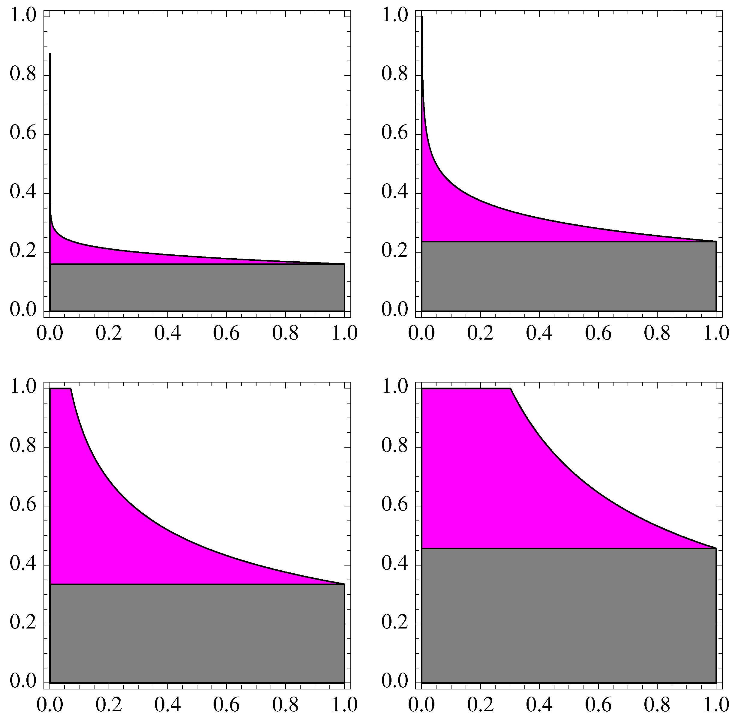
On the other hand, in Figure 2, we observe the relationship between the domains of parameters associated with Theorem 1 (gray region) and Corollary 4 (magenta region) from the variability of ε and for four different values of p: $p=\frac{1}{10},\frac{1}{5},\frac{2}{5},\frac{4}{5}$. As we can see, the domain associated with Corollary 4 is always larger, for all $\epsilon \in [0,1]$, than that associated with Theorem 1.

Figure 2. Domains of parameters of Newton’s method associated with Corollary 4 (magenta region) and Theorem 1 (gray region) for $p=\frac{1}{10},\frac{1}{5},\frac{2}{5},\frac{4}{5}$.

In addition, we prove analytically in the following what we have just seen graphically. First, we prove that ${\mathcal{D}}_{\text{T}}\subset {\mathcal{D}}_{\text{C}}^{\epsilon }$, for each $p\in (0,1]$ and $\epsilon \in [0,1]$. For this, if $(K,\beta {\eta }^p)\in {\mathcal{D}}_{\text{T}}$, then $h\le \xi \left(p\right)\le \frac{1}{2}\le \frac{1}{2\epsilon }\le \frac{1+p}{\epsilon (2+p)}$, since $p\in (0,1]$ and $\epsilon \in [0,1]$. Moreover, $h\le \xi \left(p\right)\le \xi \left(p\right)\frac{{(1+p)}^p{(1-\epsilon h)}^{1+p}}{{\epsilon }^p{h}^p}$, since $\varphi (\epsilon h;p)\ge 0$ when $h\le \xi \left(p\right)$ and $\epsilon h\le \xi \left(p\right)$. Therefore, $(K,\beta {\eta }^p)\in {\mathcal{D}}_{\text{C}}^{\epsilon }$ for each $p\in (0,1]$ and $\epsilon \in [0,1]$.

Finally, we see that ${\mathcal{D}}_{\text{C}}^{{\epsilon }_2}\subset {\mathcal{D}}_{\text{C}}^{{\epsilon }_1}$ if ${\epsilon }_1<{\epsilon }_2$ with ${\epsilon }_1,{\epsilon }_2\in [0,1]$. Indeed, from $\psi \left(\epsilon \right)=\frac{1+p}{(2+p)\epsilon }$ and $\phi \left(\epsilon \right)=\xi \left(p\right)\frac{{(1+p)}^p{(1-\epsilon h)}^{1+p}}{{\epsilon }^p{h}^p}$, we have ${\psi }^{\prime }\left(\epsilon \right)=\frac{-(1+p)}{(2+p){\epsilon }^2}\le 0$ and ${\phi }^{\prime }\left(\epsilon \right)=-\frac{{(1+p)}^p\xi \left(p\right){(1-\epsilon h)}^p(p+\epsilon h)}{{\epsilon }^{1+p}{h}^p}\le 0$, since $1-\epsilon h\ge \frac{1}{2+p}\ge 0$, so that $\psi \left({\epsilon }_2\right)\le \psi \left({\epsilon }_1\right)$ and $\phi \left({\epsilon }_2\right)\le \phi \left({\epsilon }_1\right)$, and therefore ${\mathcal{D}}_{\text{C}}^{{\epsilon }_2}\subset {\mathcal{D}}_{\text{C}}^{{\epsilon }_1}$.

To that end, we have proven the improvement obtained for the domain of parameters of Newton’s method with the help of the conditions of type (3) that we have just shown in Figure 2.

5. Application

Now, we illustrate all of that mentioned above with the following mildly nonlinear elliptic equation:

$$u_{xx}+u_{yy}=u^{5/3}.$$

(21)

This type of equation is of interest in the theory of gas dynamics [7]. An associated Dirichlet problem can be formulated as follows. Suppose that the equation is satisfied in the interior of the square $0\le x,y\le 1$ in ${\mathbb{R}}^2$ and that $u(x,y)>0$ is given and continuous on the boundary of the square ([8]):

$$\begin{array}{ccc}u(x,0)=2x^2-x+1,\hfill & u(x,1)=2,\hfill & 0\le x\le 1,\hfill \\ u(0,y)=2y^2-y+1,\hfill & u(1,y)=2,\hfill & 0\le y\le 1.\hfill \end{array}$$

(22)

Our discussion focuses on the formulation of the finite difference equation for the elliptic boundary value Problems (21)–(22). The method of finite differences applied to this problem yields a finite system of equations. For general use, iterative techniques often represent the best approach to the solution of such finite systems of equations.

Specifically, central difference approximations for (21) are used, so that Problems (21)–(22) are reduced to the problem of finding a real zero of a function $F:\Omega \subseteq {\mathbb{R}}^m⟶{\mathbb{R}}^m$, namely a real solution ${\mathbf{x}}^{*}$ of a nonlinear system $F\left(\mathbf{x}\right)=0$ with m equations and m unknowns. The common technique used to approximate ${\mathbf{x}}^{*}$ is the application of iterative methods. In this case, Newton’s method goes on being the most used iterative method for approximating ${\mathbf{x}}^{*}$, since this method is one of the most efficient.

For Problems (21)–(22) in ${\mathbb{R}}^2$, Equation (21) can be approximated using central difference approximations for the spacial derivatives. Consider a grid with step size $h=\frac{1}{N+1}$ in x and $k=\frac{1}{M+1}$ in y defined over the region D, so that D is partitioned into a grid consisting of $(N+1)\times (M+1)$ rectangles with sides $h=\frac{1}{N+1}$ and $k=\frac{1}{M+1}$. The mesh points $(x_i,y_j)$ are given by:

$$x_i=ih,y_i=jk,i=0,1,\dots ,N+1,j=0,1,\dots ,M+1.$$

Considering the following finite difference expressions to approximate the partial differentials:

$$u_{xx}(x_i,y_j)=\frac{u(x_{i-1},y_j)-2u(x_i,y_j)+u(x_{i+1},y_j)}{h^2}+\mathcal{O}\left(h^2\right),$$

$$u_{yy}(x_i,y_j)=\frac{u(x_i,y_{j-1})-2u(x_i,y_j)+u(x_i,y_{j+1})}{k^2}+\mathcal{O}\left(k^2\right),$$

Equation (21) is approximated at each interior grid point $(x_i,y_j)$ by the difference equation:

$$\frac{u(x_{i+1},y_j)-2u(x_i,y_j)+u(x_{i-1},y_j)}{h^2}+\frac{u(x_i,y_{j+1})-2u(x_i,y_j)+u(x_i,y_{j-1})}{k^2}=u{(x_i,y_j)}^{5/3},$$

for $i=1,2,\dots ,N$ and $j=1,2,\dots ,M$. The boundary conditions are:

$$\begin{array}{ccc}u(x_i,y_0)=2x_i^2-x_i+1,\hfill & u(x_i,y_M)=2,\hfill & i=1,2,\dots ,N,\hfill \\ u(x_0,y_j)=2y_j^2-y_j+1,\hfill & u(x_N,y_j)=2,\hfill & j=0,1,\dots ,M+1.\hfill \end{array}$$

If we now denote the approximate value of $u(x_i,y_j)$ as $u_{i,j}$, we obtain the difference equation:

$$2\left[{\left(\frac{h}{k}\right)}^2+1\right]u_{i,j}-(u_{i-1,j}+u_{i+1,j})-{\left(\frac{h}{k}\right)}^2(u_{i,j-1}+u_{i,j+1})=-h^2{u}_{i,j}^{5/3},$$

for $i=1,2,\dots ,N$ and $j=1,2,\dots ,M$, with:

$$\begin{array}{ccc}{u}_{i,0}=2x_i^2-x_i+1,\hfill & u_{i,M+1}=2,\hfill & i=1,2,\dots ,N,\hfill \\ u_{0,j}=2y_j^2-y_j+1,\hfill & u_{N+1,j}=2,\hfill & j=0,1,\dots ,M+1.\hfill \end{array}$$

Equation (21) with the boundary conditions given in (22) forms an $NM\times NM$ nonlinear system of equations. To set up the nonlinear system, the $NM=m$ interior grid points are labeled row-by-row from $x_1$ to $x_m$ starting from the left-bottom corner point. The resulting system is:

$$A\mathbf{x}+h^{2}q\left(\mathbf{x}\right)=\mathbf{v},$$

where:

$$A={\left(\begin{array}{cccccc}B& C& 0& \cdots & \cdots & 0\\ C& B& C& \ddots & & ⋮\\ 0& C& B& C& \ddots & ⋮\\ ⋮& \ddots & \ddots & \ddots & \ddots & 0\\ ⋮& & \ddots & \ddots & \ddots & C\\ 0& \cdots & \cdots & 0& C& B\end{array}\right)}_{M\times M},$$

$$B={\left(\begin{array}{cccccc}2(\lambda +1)& -1& 0& \cdots & \cdots & 0\\ -1& 2(\lambda +1)& -1& \ddots & & ⋮\\ 0& -1& 2(\lambda +1)& -1& \ddots & ⋮\\ ⋮& \ddots & \ddots & \ddots & \ddots & 0\\ ⋮& & \ddots & \ddots & \ddots & -1\\ 0& \cdots & \cdots & 0& -1& 2(\lambda +1)\end{array}\right)}_{N\times N},$$

$C=-\lambda I$, $\lambda ={\left(\frac{h}{k}\right)}^2$, I is the identity matrix in ${\mathbb{R}}^N$, $\mathbf{x}={(x_1,x_2,\dots ,x_m)}^t$, $q\left(\mathbf{x}\right)={\left(x_1^{5/3},x_2^{5/3},\dots ,x_m^{5/3}\right)}^t$ and $\mathbf{v}$ is a vector formed from the boundary conditions (systems of this type are so-called mildly nonlinear systems).

If we denote the previous system by $F\left(\mathbf{x}\right)=0$, where:

$$F\left(\mathbf{x}\right)=A\mathbf{x}+h^{2}q\left(\mathbf{x}\right)-\mathbf{v}\text{and}F:{\mathbb{R}}^m⟶{\mathbb{R}}^m,m=NM,$$

(23)

then $F^{\prime }\left(\mathbf{x}\right)$ is a linear operator, which is given by the matrix:

$$F^{\prime }\left(\mathbf{x}\right)=A+h^{2}Q\left(\mathbf{x}\right),Q\left(\mathbf{x}\right)=\frac{5}{3}\text{diag}\left\{x_1^{2/3},x_2^{2/3},\dots ,x_m^{2/3}\right\}.$$

(24)

We now choose $N=M=4$ and the infinity norm. In addition, the number of equations is $m=16$, $h=k=\frac{1}{5}$ and $\lambda =1$. Besides, $q\left(\mathbf{x}\right)={\left(x_1^{5/3},x_2^{5/3},\dots ,x_{16}^{5/3}\right)}^t$ and:

$$\mathbf{v}={\left(\frac{44}{25},\frac{23}{25},\frac{28}{25},\frac{87}{25},\frac{23}{25},0,0,2,\frac{28}{25},0,0,2,\frac{87}{25},2,2,4\right)}^t.$$

In this case, we observe that a solution ${\mathbf{x}}^{*}$ of the system $F\left(x\right)=0$ with F defined in (23) satisfies:

$$\parallel {\mathbf{x}}^{*}\parallel \le \parallel A^{-1}\parallel \left(\parallel \mathbf{v}\parallel +h^2\parallel q\left(\mathbf{x}\right)\parallel \right)\Rightarrow \parallel {\mathbf{x}}^{*}\parallel -\frac{5}{3}\left(4+\frac{1}{25}{\parallel {\mathbf{x}}^{*}\parallel }^{5/3}\right)\le 0,$$

where $\parallel A^{-1}\parallel =\frac{5}{3}$ and $\parallel \mathbf{v}\parallel =4$, so that $\parallel {\mathbf{x}}^{*}\parallel \in [0,{\varrho }_1]\cup [{\varrho }_2,+\infty ]$, where ${\varrho }_1=9.5149\dots$ and ${\varrho }_2=45.9125\dots$ are the two positive real roots of the scalar equation $t-\frac{5}{3}\left(4+\frac{t^{5/3}}{25}\right)=0$. Then, we can consider:

$$F:\Omega \subset {\mathbb{R}}^{16}⟶{\mathbb{R}}^{16}\text{with}\Omega =\left\{\mathbf{x}\in {\mathbb{R}}^{16}:\parallel \mathbf{x}\parallel <10\right\},$$

since ${\varrho }_1<10<{\varrho }_2$.

Moreover, $F^{\prime }\left(\mathbf{x}\right)$ is the linear operator given by the matrix:

$$A+\frac{1}{15}\text{diag}\left\{x_1^{2/3},x_2^{2/3},\dots ,x_{16}^{2/3}\right\}$$

and:

$$F^{\prime }\left(\mathbf{x}\right)-F^{\prime }\left(\mathbf{y}\right)=\frac{1}{15}\text{diag}\left\{x_1^{2/3}-y_1^{2/3},x_2^{2/3}-y_2^{2/3},\dots ,x_{16}^{2/3}-y_{16}^{2/3}\right\},$$

where $\mathbf{y}={(y_1,y_2,\dots ,y_{16})}^t$. In addition,

$$\begin{array}{cc}\hfill \parallel F^{\prime }\left(\mathbf{x}\right)-F^{\prime }\left(\mathbf{y}\right)\parallel & \le \frac{1}{15}∥{\mathbf{x}}^{1/3}+{\mathbf{y}}^{1/3}∥∥{\mathbf{x}}^{1/3}-{\mathbf{y}}^{1/3}∥\le \frac{2}{15}\sqrt[3]{10}{\parallel \mathbf{x}-\mathbf{y}\parallel }^{1/3},\hfill \\ \hfill \parallel F^{\prime }\left(\mathbf{x}\right)-F^{\prime }\left({\mathbf{x}}_{\mathbf{0}}\right)\parallel & \le \frac{1}{15}\left({\parallel \mathbf{x}\parallel }^{1/3}+{\parallel {\mathbf{x}}_{\mathbf{0}}\parallel }^{1/3}\right)\parallel \mathbf{x}-{\mathbf{x}}_{\mathbf{0}}{\parallel }^{1/3}\le \frac{1}{15}\left(\sqrt[3]{10}+{\parallel {\mathbf{x}}_{\mathbf{0}}\parallel }^{1/3}\right){\parallel \mathbf{x}-{\mathbf{x}}_{\mathbf{0}}\parallel }^{1/3}.\hfill \end{array}$$

Thus, $K=0.2872\dots$, $K_0=0.2199\dots$ and $p=\frac{1}{3}$.

If we choose the starting point ${\mathbf{x}}_{\mathbf{0}}={\left(\frac{3}{2},\frac{3}{2},\dots ,\frac{3}{2}\right)}^t$, we obtain $\beta =1.4862\dots$ and $\eta =0.5185\dots$, so that the condition $h=K\beta {\eta }^p\le \xi \left(p\right)$ of Theorem 1 is not satisfied, since $h=0.3429\dots >\xi \left(p\right)=\xi \left(\frac{1}{3}\right)=0.3071\dots$, where $\xi \left(\frac{1}{3}\right)$ is the unique zero of the corresponding auxiliary function given by (2), $\varphi \left(x;\frac{1}{3}\right)=\frac{1}{3}\left(6^{2/3}{(1-t)}^{4/3}-3\sqrt[3]{t}\right)$, in the interval $\left(0,\frac{1}{2}\right]$. As a consequence, we cannot use Theorem 1 to guarantee the convergence of Newton’s method for approximating a solution of the system $F\left(\mathbf{x}\right)=0$, where F is defined in (23).

However, we can guarantee the convergence of Newton’s method from Corollary 4, since Condition (20) is satisfied: $h=0.3429\dots <\xi \left(p\right)\frac{{(1+p)}^p{(1-\epsilon h)}^{1+p}}{{\epsilon }^p{h}^p}=0.3517\dots$ with $\epsilon =0.7656\dots$. Therefore, we can then apply Newton’s method for approximating a solution of the system $F\left(\mathbf{x}\right)=0$ with F defined in (23) and obtain the approximation given by the vector ${\mathbf{x}}^{*}={(x_1^{*},x_2^{*},\dots ,x_{16}^{*})}^t$ that is shown in Table 1, reached after four iterations with a tolerance ${10}^{-16}$. In Table 2, we show the errors $\parallel {\mathbf{x}}_{\mathbf{n}}-{\mathbf{x}}^{*}\parallel$ using the stopping criterion $\parallel {\mathbf{x}}_{\mathbf{n}}-{\mathbf{x}}_{\mathbf{n}-\mathbf{1}}\parallel <{10}^{-16}$. Notice that the vector shown in Table 1 is a good approximation of the solution of the system, since $\parallel F\left({\mathbf{x}}^{*}\right)\parallel \le C\times {10}^{-16}$. See the sequence $\{\parallel F\left({\mathbf{x}}_{\mathbf{n}}\right)\parallel \}$ in Table 2.

Table 1. Approximation of the solution ${\mathbf{x}}^{*}$ of $F\left(\mathbf{x}\right)=0$ with F given in (23).

i	$x_i^{*}$	i	$x_i^{*}$	i	$x_i^{*}$	i	$x_i^{*}$
1	$0.979069\dots$	5	$1.097445\dots$	9	$1.291651\dots$	13	$1.587503\dots$
2	$1.097445\dots$	6	$1.245767\dots$	10	$1.422935\dots$	14	$1.664776\dots$
3	$1.291651\dots$	7	$1.422935\dots$	11	$1.561551\dots$	15	$1.742203\dots$
4	$1.587503\dots$	8	$1.664776\dots$	12	$1.742203\dots$	16	$1.843388\dots$

Table 1. Approximation of the solution ${\mathbf{x}}^{*}$ of $F\left(\mathbf{x}\right)=0$ with F given in (23).

i	$x_i^{*}$	i	$x_i^{*}$	i	$x_i^{*}$	i	$x_i^{*}$
1	$0.979069\dots$	5	$1.097445\dots$	9	$1.291651\dots$	13	$1.587503\dots$
2	$1.097445\dots$	6	$1.245767\dots$	10	$1.422935\dots$	14	$1.664776\dots$
3	$1.291651\dots$	7	$1.422935\dots$	11	$1.561551\dots$	15	$1.742203\dots$
4	$1.587503\dots$	8	$1.664776\dots$	12	$1.742203\dots$	16	$1.843388\dots$

Table 2. Absolute errors obtained by Newton’s method and $\{\parallel F\left({\mathbf{x}}_{\mathbf{n}}\right)\parallel \}$.

n	$\parallel x_n-x^{*}\parallel$	$\parallel F\left(x_n\right)\parallel$
0	$5.2093\dots \times {10}^{-1}$	$1.318622\dots$
1	$2.4028\dots \times {10}^{-3}$	$5.4477\dots \times {10}^{-3}$
2	$8.4485\dots \times {10}^{-8}$	$1.2913\dots \times {10}^{-7}$
3	$1.2409\dots \times {10}^{-16}$	$1.4741\dots \times {10}^{-16}$

Table 2. Absolute errors obtained by Newton’s method and $\{\parallel F\left({\mathbf{x}}_{\mathbf{n}}\right)\parallel \}$.

n	$\parallel x_n-x^{*}\parallel$	$\parallel F\left(x_n\right)\parallel$
0	$5.2093\dots \times {10}^{-1}$	$1.318622\dots$
1	$2.4028\dots \times {10}^{-3}$	$5.4477\dots \times {10}^{-3}$
2	$8.4485\dots \times {10}^{-8}$	$1.2913\dots \times {10}^{-7}$
3	$1.2409\dots \times {10}^{-16}$	$1.4741\dots \times {10}^{-16}$

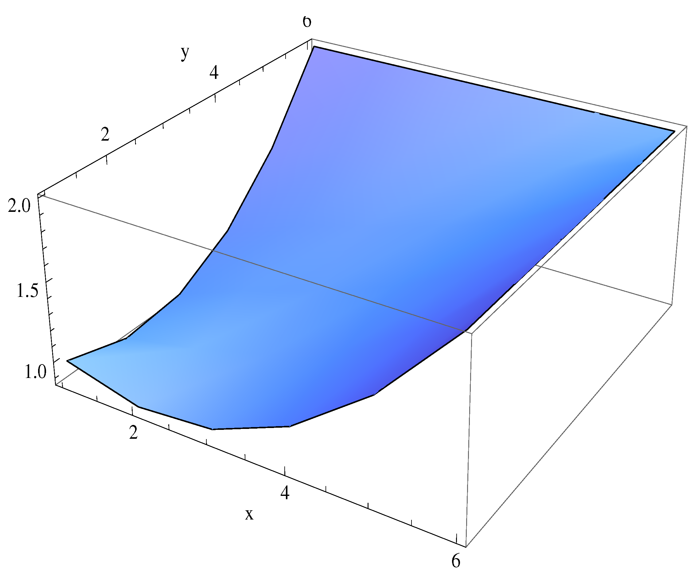
Finally, we note that if we interpolate the points of Table 1 and take into account that the solution satisfies the boundary conditions given in (22), we obtain the approximation of the numerical solution shown in Figure 3.

Figure 3. Approximated solution of Problems (21)–(22).