Article

Model Equivalence-Based Identification Algorithm for Equation-Error Systems with Colored Noise

Key Laboratory of Advanced Process Control for Light Industry (Ministry of Education), Jiangnan University, Wuxi 214122, China
*
Author to whom correspondence should be addressed.
Algorithms 2015, 8(2), 280-291; https://doi.org/10.3390/a8020280
Submission received: 1 May 2015 / Accepted: 19 May 2015 / Published: 2 June 2015

Abstract

:
For equation-error autoregressive (EEAR) systems, this paper proposes an identification algorithm by means of the model equivalence transformation. The basic idea is to eliminate the autoregressive term in the model using the model transformation, to estimate the parameters of the converted system and further to compute the parameter estimates of the original system using the comparative coefficient way and the model equivalence principle. For comparison, the recursive generalized least squares algorithm is given simply. The simulation results verify that the proposed algorithm is effective and can produce more accurate parameter estimates.

1. Introduction

System modeling and system identification are the prerequisite and foundation of all control issues. System identification has a significant effect on the filtering [13], state estimation [46], system control [79] and optimization [10]. For example, Scarpiniti et al. proposed a nonlinear filtering approach based on spline nonlinear functions [11]; Zhuang et al. presented an algorithm to estimate the parameters and states for linear systems with canonical state-space descriptions [12]; Khan et al. discussed the theoretical implementation of robust attitude estimation for a rigid spacecraft system under measurement loss [13]. As system identification becomes widely available, many identification methods have been raised, e.g., the gradient identification methods [14,15], the hierarchical identification methods [1618], the auxiliary model identification methods [19,20] and the multi-innovation identification methods [21].
In all of these identification methods, the recursive identification [2224] and the iterative identification methods [2527] constitute two categories of important parameter estimation methods [28]. The variable of the recursive identification is about time, so it can be used to estimate the system parameters online. Yu et al. derived the recursive identification algorithm to identify the parameters in the parameterized Hammerstein–Wiener system model [29]; Filipovic presented a robust recursive algorithm for identification of a Hammerstein model with a static nonlinear block in polynomial form and a linear block described by the ARMAX model [30]; Cao et al. studied constrained two-dimensional recursive least squares identification problems for batch processes, which can improve the identification performance by incorporating a soft constraint term in the cost function to reduce the variation of the estimated parameters [31]. Liu and Lu derived the mathematical models and presented a least squares-based iterative algorithm for multi-input multirate systems with colored noises by replacing the unknown noise terms in the information vector with their estimates [32].
Some estimation methods focus on the estimation problems of equation error type systems [3335], including the equation-error autoregressive (EEAR) systems, the equation-error moving average systems and the equation-error autoregressive moving average systems. For example, Xiao and Yue derived a filtering-based recursive least squares identification algorithm for nonlinear dynamical adjustment models [36]; Li developed a maximum likelihood estimation algorithm to estimate the parameters of Hammerstein nonlinear CARARMA systems by using the Newton iteration [37]; Ding presented a recursive generalized extended least squares algorithm for identifying controlled ARMA systems [28]; the basic idea is to replace the unknown terms in the information vector with their estimates. On the basis of the work in [28,32], the objective of this paper is to develop new identification algorithms using the model equivalent transformation and to provide more accurate parameter estimates.
The rest of this paper is organized as follows. Section 2 gives the identification model for EEAR systems. Section 3 gives a recursive generalized least squares algorithm, and Section 4 gives a model equivalence-based recursive least squares algorithm. Section 5 computes the parameter estimates of the original system. Section 6 provides numerical examples to prove the validity of the proposed algorithms. Finally, some concluding remarks are made in Section 7.

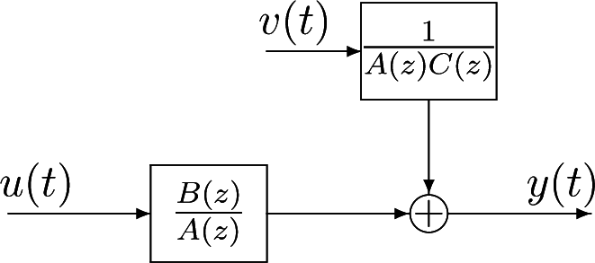
2. The Identification Model for an EEAR System

Let us define some notation. “A =: X” or “X := A” represents “A is defined as X”; the superscript T denotes the matrix/vector transpose; the norm of a matrix X is defined by ||X||2 := tr[XXT]; I stands for an identity matrix of appropriate size; X ^ ( t ) represents the estimate of X at time t.
Consider the following equation-error autoregressive system, i.e., the controlled autoregressive autoregressive (CARAR) system, in Figure 1,
A ( z ) y ( t ) = B ( z ) u ( t ) + 1 C ( z ) v ( t )
where u(t) and y(t) are the measured input and output of the system, respectively, v(t) represents stochastic white noise with zero mean and variance σ2 and A(z), B(z) and C(z) denote the polynomials in the unit backward shift operator z1 [i.e., z1y(t) = y(t − 1)]:
A ( z ) : = 1 + a 1 z 1 + a 2 z 2 + + a n a z n a , B ( z ) : = b 1 z 1 + b 2 z 2 + + b n b z n b , C ( z ) : = 1 + c 1 z 1 + c 2 z 2 + + c n c z n c
Suppose that u(t) = 0, y(t) = 0, v(t) = 0 for t ⩽ 0, the orders na, nb and nc are known, and n := na + nb + nc.
Define the intermediate variable (the correlated stochastic noise):
w ( t ) : = 1 C ( z ) v ( t )
Inserting Equation (2) into Equation (1) yields
A ( z ) y ( t ) = B ( z ) u ( t ) + w ( t )
Define the parameter vector θs and the information vector φ s(t) of the system model and the parameter vector θn and the information vector φ n(t) of the noise model as
θ : = [ θ s θ n ] n , θ s : = [ a 1 , a 2 , , a n a , b 1 , b 2 , , b n b ] T n a + n b , θ n : = [ c 1 , c 2 , , c n c ] T n c , φ ( t ) : = [ φ s ( t ) φ n ( t ) ] n , φ s ( t ) : = [ y ( t 1 ) , y ( t 2 ) , , y ( t n a ) , u ( t 1 ) , u ( t 2 ) , , u ( t n b ) ] T n a + n b , φ n ( t ) : = [ w ( t 1 ) , w ( t 2 ) , , w ( t n c ) ] T n c
where subscripts s and n denote the first letters of the words “system” and “noise”, respectively. φs(t) is the known information vector, which consists of measured input-output data u(t − i) and y(t − i); φn(t) is the unknown information vector, which consists of noise terms w(t − i). By means of the above definitions, Equations (2) and (3) can be expressed as:
w ( t ) = [ 1 C ( z ) ] w ( t ) + v ( t ) = φ n T ( t ) θ n + v ( t ) y ( t ) = [ 1 A ( z ) ] y ( t ) + B ( z ) u ( t ) + w ( t ) = φ s T ( t ) θ s + w ( t ) = φ T ( t ) θ + v ( t )
This is the identification model for the EEAR system in Equation (1). The objective of this paper is to propose new identification algorithms for estimating the parameters of EEAR systems.

3. The Recursive Generalized Least Squares Algorithm

As we all know, the recursive generalized least squares algorithm can identify CARAR systems [36].
The core idea is to substitute their estimates for the unmeasurable noise terms in the information vector. The following is the recursive generalized least squares (RGLS) algorithm for estimating the parameter vector θ of the EEAR systems:
θ ^ ( t ) = θ ^ ( t 1 ) + L 1 ( t ) [ y ( t ) φ ^ T ( t ) θ ^ ( t 1 ) ]
L 1 ( t ) = P 1 ( t 1 ) φ ^ ( t ) [ 1 + φ ^ T ( t ) P 1 ( t 1 ) φ ^ ( t ) ] 1
P 1 ( t ) = [ I L 1 ( t ) φ ^ T ( t ) ] P 1 ( t 1 ) , P 1 ( 0 ) p 0 I
φ ^ ( t ) = [ φ s ( t ) φ ^ n ( t ) ] , θ ^ ( t ) = [ θ ^ s ( t ) θ ^ n ( t ) ]
φ s ( t ) : = [ y ( t 1 ) , y ( t 2 ) , , y ( t n a ) , u ( t 1 ) , u ( t 2 ) , , u ( t n b ) ] T
φ ^ n ( t ) : = [ w ^ ( t 1 ) , w ^ ( t 2 ) , , w ^ ( t n c ) ] T
w ^ ( t ) = y ( t ) φ s T ( t ) θ ^ s ( t )
θ ^ s ( t ) : = [ a ^ 1 ( t ) , a ^ 2 ( t ) , , a ^ n a ( t ) , b ^ 1 ( t ) , b ^ 2 ( t ) , , b ^ n b ( t ) ] T
θ ^ n ( t ) : = [ c ^ 1 ( t ) , c ^ 2 ( t ) , , c ^ n c ( t ) ] T
The RGLS algorithm can estimate the parameters of EEAR systems on-line.

4. The Model Equivalence-Based Recursive Least Squares Algorithm

For the EEAR system in Equation (1), the information vector φ(t) of the recursive generalized least squares algorithm contains the unknown noise terms w(t − i). The solution is replacing the unknown noise terms w(t − i) with their estimates. However, the existence of the unknown noise terms in the information vector φ(t) affects the accuracy of the parameter estimates to some extent.
The method proposed in this paper is transforming the original system with colored noise into an equation-error system using the model equivalent transformation, so that the information vector in the identification model is composed of the available input u(t − i) and output y(t − i). Since there are no noise terms to be estimated in the information vector, the identification accuracy can be improved.
Consider the CARAR system in Figure 1, which is rewritten as follows,
A ( z ) y ( t ) = B ( z ) u ( t ) + 1 C ( z ) v ( t )
Multiplying both sides of it by C(z) makes
A ( z ) C ( z ) y ( t ) = B ( z ) C ( z ) u ( t ) + v ( t )
For simplicity, let np := na + nc and nq := nb + nc; define the polynomials:
P ( z ) : = C ( z ) A ( z ) = 1 + p 1 z 1 + p 2 z 2 + + p n p z n p
Q ( z ) : = C ( z ) B ( z ) = q 1 z 1 + q 2 z 2 + + q n q z n q
Inserting Equations (16) and (17) into Equation (15) yields
P ( z ) y ( t ) = Q ( z ) u ( t ) + v ( t )
It is clear that Equation (14) reduces to an equation-error model, whose parameters can be estimated by the recursive least squares algorithm. Define the parameter vector ϑ and the information vector ϕ (t) as
ϑ : = [ p 1 , p 2 , , p n p , q 1 , q 2 , , q n q ] T n p + n q ϕ ( t ) : = [ y ( t 1 ) , y ( t 2 ) , , y ( t n p ) , u ( t 1 ) , u ( t 2 ) , , u ( t n q ) ] T n p + n q
In this case, Equation (18) can be equivalently written as
y ( t ) = ϕ T ( t ) ϑ + v ( t )
That is the identification model of Equation (18). Let ϑ ^ ( t ) be the estimate of ϑ at time t. We obtain the recursive least squares algorithm for identifying ϑ in Equation (19):
ϑ ^ ( t ) = ϑ ^ ( t 1 ) + L 2 ( t ) [ y ( t ) ϕ T ( t ) ϑ ^ ( t 1 ) ]
L 2 ( t ) = P 2 ( t 1 ) ϕ ( t ) [ 1 + ϕ T ( t ) P 2 ( t 1 ) ϕ ( t ) ] 1
P 2 ( t ) = [ I L 2 ( t ) ϕ T ( t ) ] P 2 ( t 1 ) , P 2 ( 0 ) p 0 I
v ^ ( t ) = y ( t ) ϕ T ( t ) ϑ ^ ( t )
ϕ ( t ) : = [ y ( t 1 ) , y ( t 2 ) , , y ( t n p ) , u ( t 1 ) , u ( t 2 ) , , u ( t n q ) ] T
ϑ ^ ( t ) : = [ p ^ 1 ( t ) , p ^ 2 ( t ) , , p ^ n p ( t ) , q ^ 1 ( t ) , q ^ 2 ( t ) , , q ^ n q ( t ) ] T
From Equations (20)–(25), we can compute the parameter estimate ϑ ^ ( t ), i.e., the estimates of the parameters pi and qi. The following derives the model equivalence-based recursive least squares algorithm.

5. The Parameter Estimation of the Original System

According to the acquired estimates p ^ i ( t ) and q ^ i ( t ) of the parameters pi and qi, we can compute the parameter estimates âi(t), b ^ i ( t ) and ĉi(t) of the original system. The key idea is using the coefficient equivalent principle, and the details are as follows.
Assume that the estimates of A(z), B(z) and C(z) are
A ^ ( t , z ) : = 1 + a ^ 1 ( t ) z 1 + a ^ 2 ( t ) z 2 + + a ^ n a ( t ) z n a , B ^ ( t , z ) : = b ^ 1 ( t ) z 1 + b ^ 2 ( t ) z 2 + + b ^ n b ( t ) z n b , C ^ ( t , z ) : = 1 + c ^ 1 ( t ) z 1 + c ^ 2 ( t ) z 2 + + c ^ n c ( t ) z n c
According to Equations (16) and (17), we can approximately suppose
P ^ ( t , z ) : = C ^ ( t , z ) A ^ ( t , z ) = 1 + p ^ 1 ( t ) z 1 + p ^ 2 ( t ) z 2 + + p ^ n p ( t ) z n p
Q ^ ( t , z ) : = C ^ ( t , z ) B ^ ( t , z ) = q ^ 1 ( t ) z 1 + q ^ 2 ( t ) z 2 + + q ^ n q ( t ) z n q
Based on the above assumptions, we let
B ^ ( t , z ) P ^ ( t , z ) = A ^ ( t , z ) Q ^ ( t , z )
Using B ^ ( t , z ), P ^ ( t , z ), Â(t, z) and Q ^ ( t , z ) gives
[ b ^ 1 ( t ) z 1 + + b ^ n b ( t ) z n b ] [ 1 + p ^ 1 ( t ) z 1 + + p ^ n p ( t ) z n p ] = [ 1 + a ^ 1 ( t ) z 1 + + a ^ n a ( t ) z n a ] [ q ^ 1 ( t ) z 1 + + q ^ n p ( t ) z n p ]
Expanding the above equation and comparing the coefficients of the same power of z1 on both sides, we can set up (nb + np) equations:
z 1 : b ^ 1 ( t ) = q ^ 1 ( t ) , z 2 : b ^ 1 ( t ) p ^ 1 ( t ) + b ^ 2 ( t ) = q ^ 1 ( t ) a ^ 1 ( t ) + q ^ 2 ( t ) , z 3 : b ^ 1 ( t ) p ^ 2 ( t ) + b ^ 2 ( t ) p ^ 1 ( t ) + b ^ 3 ( t ) = q ^ 1 ( t ) a ^ 2 ( t ) + q ^ 2 ( t ) a ^ 1 ( t ) + q ^ 3 ( t ) , z ( n b + n p ) + 1 : b ^ n b 1 ( t ) p ^ n p ( t ) + b ^ n b ( t ) p ^ n p 1 ( t ) = q ^ n q 1 ( t ) a ^ n a ( t ) + q ^ n q ( t ) a ^ n a 1 ( t ) , z ( n b + n p ) : b ^ n b ( t ) p ^ n p ( t ) = q ^ n q ( t ) a ^ n a ( t )
which can be written in a matrix form,
S ( t ) ϑ ^ 1 ( t ) = B ( t )
where
S ( t ) : = [ S p ( t ) , S q ( t ) ] ( n b + n p ) × ( n a + n b ) , ϑ ^ 1 ( t ) : = [ b ^ 1 ( t ) , b ^ 2 ( t ) , , b ^ n b ( t ) , a ^ 1 ( t ) , a ^ 2 ( t ) , , a ^ n a ( t ) ] T n a + n b , S p ( t ) : = [ 1 0 0 p ^ 1 ( t ) 1 p ^ 2 ( t ) p ^ 1 ( t ) 1 p ^ 2 ( t ) p ^ 1 ( t ) 0 p ^ n p 1 ( t ) 1 p ^ n p ( t ) p ^ n p 1 ( t ) p ^ 1 ( t ) 0 p ^ n p ( t ) p ^ 2 ( t ) p ^ n p 1 ( t ) p ^ n p ( t ) p ^ n p 1 ( t ) 0 0 p ^ n p ( t ) ] ( n b + n p ) × n b , B ( t ) : = [ q ^ 1 ( t ) q ^ 2 ( t ) q ^ n q ( t ) 0 0 0 ] n b + n p , S q ( t ) : = [ 0 0 0 q ^ 1 ( t ) 0 q ^ 2 ( t ) q ^ 1 ( t ) 0 q ^ 2 ( t ) q ^ 1 ( t ) 0 q ^ n q 1 ( t ) 0 q ^ n q ( t ) q ^ n q 1 ( t ) q ^ 1 ( t ) 0 q ^ n q ( t ) q ^ 2 ( t ) q ^ n q 1 ( t ) q ^ n q ( t ) q ^ n q 1 ( t ) 0 0 q ^ n q ( t ) ] ( n b + n p ) × n a
It is easy to know that
ϑ ^ 1 ( t ) = [ S T ( t ) S ( t ) ] 1 S T ( t ) B ( t )
From Equation (29), we can get the estimates âi(t) and b ^ i ( t ) of parameters ai and bi from ϑ ^ 1 ( t ). According to the definition of P ^ ( t , z ) in Equation (26), similarly, expanding the equation and comparing the coefficients on both sides of it gives the matrix equation,
S 1 ( t ) ϑ ^ 2 ( t ) = B 1 ( t )
where
ϑ ^ 2 ( t ) : = [ c ^ 1 ( t ) , c ^ 2 ( t ) , , c ^ n c ( t ) ] T n c , B 1 ( t ) : = [ p ^ 1 ( t ) a ^ 1 ( t ) p ^ 2 ( t ) a ^ 2 ( t ) p ^ n a ( t ) a ^ n a ( t ) p ^ n a + 1 ( t ) p ^ n a + 2 ( t ) p ^ n p ( t ) ] n p , S 1 ( t ) : = [ 1 0 0 a ^ 1 ( t ) 1 a ^ 2 ( t ) a ^ 1 ( t ) 1 a ^ 2 ( t ) a ^ 1 ( t ) 0 a ^ n a 1 ( t ) 1 a ^ n a ( t ) a ^ n a 1 ( t ) a ^ 1 ( t ) 0 a ^ n a ( t ) a ^ 2 ( t ) a ^ n a 1 ( t ) a ^ n a ( t ) a ^ n a 1 ( t ) 0 0 a ^ n a ( t ) ] n p × n c
Then, we obtain
ϑ ^ 2 ( t ) = [ S 1 T ( t ) S 1 ( t ) ] 1 S 1 T ( t ) B 1 ( t )
Based on Equation (30), we can obtain the estimates ĉi(t) of ci from ϑ ^ 2 ( t ). Hence, we obtain all of the parameter estimates âi(t), b ^ i ( t ) and ĉi(t).
According to the above derivation, it is clear that the model equivalence-based recursive least squares (ME-RLS) algorithm in Equations (20)–(25) and (29)–(30) increases the complexity of computation compared with the RGLS algorithm. However, as the information vector of the ME-RLS algorithm does not contain noise vectors to be estimated, the estimation errors become smaller.

6. Numerical Example

Consider the following CARAR system,
A ( z ) y ( t ) = B ( z ) u ( t ) + 1 C ( z ) v ( t ) , A ( z ) = 1 + a 1 z 1 + a 2 z 2 = 1 1.60 z 1 + 0.66 z 2 , B ( z ) = b 1 z 1 + b 2 z 2 = 0.64 z 1 0.34 z 2 , C ( z ) = 1 + c 1 z 1 + c 2 z 2 = 1 0.55 z 1 + 0.47 z 2 , θ = [ a 1 , a 2 , b 1 , b 2 , c 1 , c 2 ] T = [ 1.60 , 0.66 , 0.64 , 0.34 , 0.55 , 0.47 ] T
Here, the input {u(t)} is taken as an uncorrelated persistent excitation signal sequence with zero mean and unit variance, {v(t)} is a stochastic white noise sequence with zero mean and variances σ2 = 0.102 and is independent of the input {u(t)}.
Using the model equivalence-based recursive least squares (ME-RLS) algorithm and the recursive generalized least squares (RGLS) algorithm to estimate the parameters of this system, the parameter estimates and their errors are shown in Tables 13, and the estimation errors δ versus the data length t are shown in Figure 2, where δ 1 : = | | ϑ ^ ( t ) ϑ | | / | | ϑ | | and δ 2 : = | | θ ^ ( t ) θ | | / | | θ | | are the estimation errors of the ME-RLS algorithm and the RGLS algorithm, when σ2 = 0.102; the system noise-to-signal ratio is δns = 35.01%.
From Tables 13 and Figure 2, we can obtain the following conclusions.
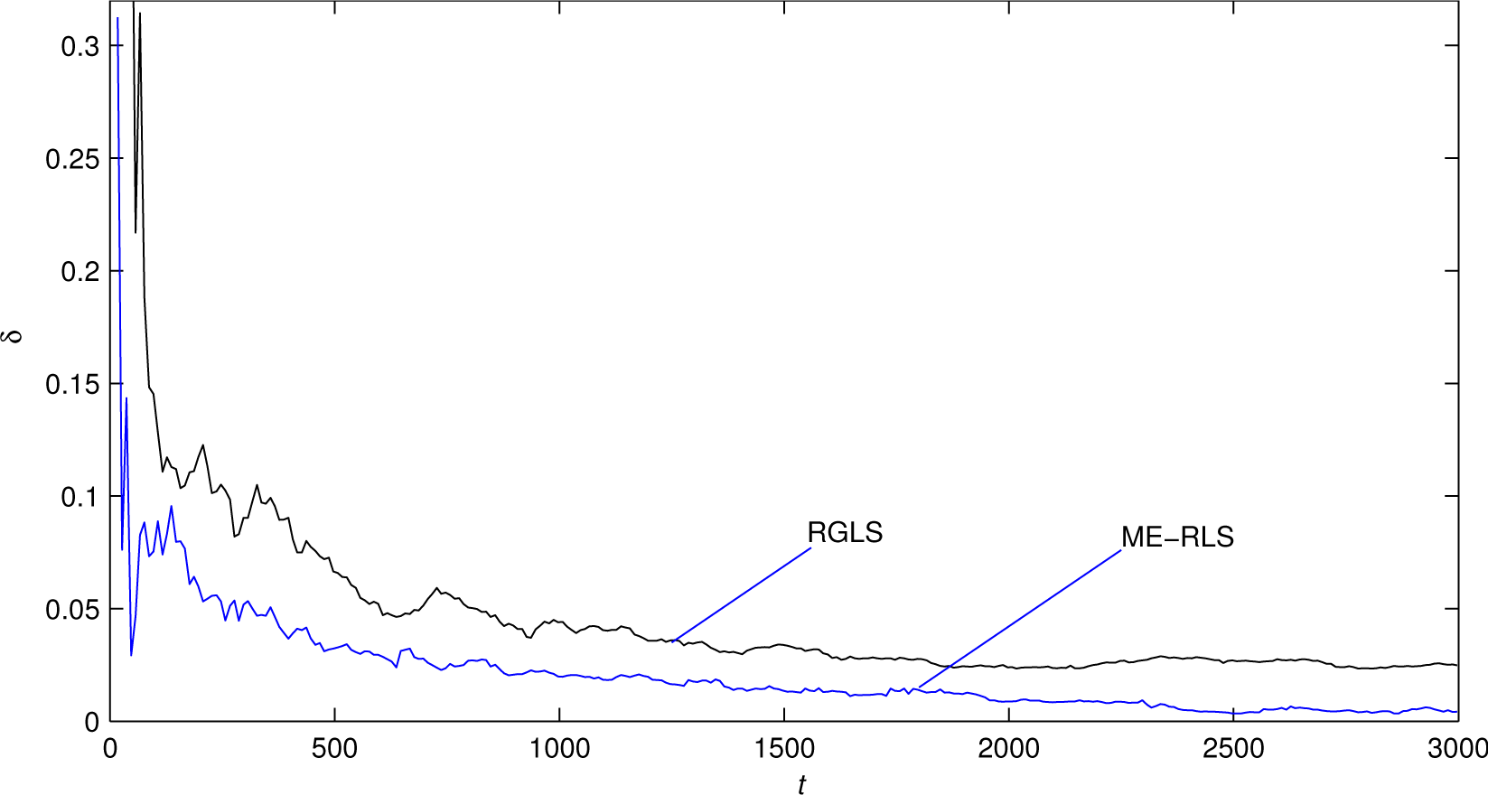
  • The estimation errors of the ME-RLS algorithm become smaller, and the estimates converge to their true values with the data length increasing (i.e., the proposed algorithm works well).
  • The estimation errors of the ME-RLS algorithm are smaller than those of the RGLS algorithm, which means that the parameter estimates given by the ME-RLS algorithm have higher accuracy than the RGLS algorithm for CARAR systems.

7. Conclusions

This paper derives the recursive least squares algorithm based on the model transformation principle for CARAR. Compared with the LS identification algorithms, the algorithms presented in this paper reduce the number of the noise items to be estimated, and so, can generate more accurate parameter estimates. The proposed algorithm can be used to study the identification problems for other systems with autoregressive items.

Acknowledgments

This work was supported by the National Science Foundation of China (No. 61273194) and the PAPDof Jiangsu Higher Education Institutions.

Author Contributions

Joint work.

Conflicts of Interest

The authors declare no conflict of interest.

References

  1. Scarpiniti, M.; Comminiello, D.; Parisi, R.; Uncini, A. Nonlinear system identification using IIR Spline Adaptive Filtering. Signal Process. 2015, 108, 30–35. [Google Scholar]
  2. Li, H.; Shi, Y. Robust H-infty filtering for nonlinear stochastic systems with uncertainties and random delays modeled by Markov chains. Automatica 2012, 48, 159–166. [Google Scholar]
  3. Zhang, L.; Wang, Z.P.; Sun, F.C.; Dorrell, D.G. Online parameter identification of ultracapacitor models using the extended kalman filter. Algorithms 2014, 7, 3204–3217. [Google Scholar]
  4. Viegas, D.; Batista, P.; Oliveira, P.; Silvestre, C.; Chen, C.L.P. Distributed state estimation for linear multi-agent systems with time-varying measurement topology. Automatica 2015, 54, 72–79. [Google Scholar]
  5. Fang, H.; Wu, J.; Shi, Y. Genetic adaptive state estimation with missing input/output data. Proc. Inst. Mech. Eng. Part I: J. Syst. Control Eng. 2010, 224, 611–617. [Google Scholar]
  6. Fang, H.Z.; Shi, Y.; Yi, J.G. On stable simultaneous input and state estimation for discrete-time linear systems. Int. J. Adapt. Control Signal Process. 2011, 25, 671–686. [Google Scholar]
  7. Chen, F.W.; Garnier, H.; Gilson, M. Robust identification of continuous-time models with arbitrary time-delay from irregularly sampled data. J. Process Control 2015, 25, 19–27. [Google Scholar]
  8. Na, J.; Yang, J.; Wu, X.; Guo, Y. Robust adaptive parameter estimation of sinusoidal signals. Automatica 2015, 53, 376–384. [Google Scholar]
  9. Rincón, F.D.; Roux, G.A.C.L.; Lima, F.V. A novel ARX-based approach for the steady-state identification analysis of industrial depropanizer column datasets. Algorithms 2015, 3, 257–285. [Google Scholar]
  10. Upadhyay, P.; Kar, R.; Mandal, D.; Ghoshal, S.P.; Mukherjee, V. A novel design method for optimal IIR system identification using opposition based harmony search algorithm. J. Frankl. Inst. 2014, 351, 2454–2488. [Google Scholar]
  11. Scarpiniti, M.; Comminiello, D.; Parisi, R.; Uncini, A. Nonlinear spline adaptive filtering. Signal Process. 2013, 93, 772–783. [Google Scholar]
  12. Zhuang, L.F.; Pan, F.; Ding, F. Parameter and state estimation algorithm for single-input single-output linear systems using the canonical state space models. Appl. Math. Model. 2012, 36, 3454–3463. [Google Scholar]
  13. Khan, N.; Khattak, M.I.; Gu, D. Robust state estimation and its application to spacecraft control. Automatica 2012, 48, 3142–3150. [Google Scholar]
  14. Ding, F.; Liu, X.P.; Liu, G. Gradient based and least-squares based iterative identification methods for OE and OEMA systems. Digit. Signal Process. 2010, 20, 664–677. [Google Scholar]
  15. Ma, X.Y.; Ding, F. Gradient-based parameter identification algorithms for observer canonical state space systems using state estimates. Circuits Syst. Signal Process. 2015, 34, 1697–1709. [Google Scholar]
  16. Cao, Y.N.; Liu, Z.Q. Signal frequency and parameter estimation for power systems using the hierarchical dentification principle. Math. Comput. Model. 2010, 51, 854–861. [Google Scholar]
  17. Ding, F. Hierarchical parameter estimation algorithms for multivariable systems using measurement information. Inf. Sci. 2014, 227, 396–405. [Google Scholar]
  18. Liu, Y.J.; Ding, F.; Shi, Y. Least squares estimation for a class of non-uniformly sampled systems based on the hierarchical identification principle. Circuits Syst. Signal Process. 2012, 31, 1985–2000. [Google Scholar]
  19. Ding, J.; Fan, C.X.; Lin, J.X. Auxiliary model based parameter estimation for dual-rate output error systems with colored noise. Appl. Math. Model. 2013, 37, 4051–4058. [Google Scholar]
  20. Liu, Y.J.; Xiao, Y.S.; Zhao, X.L. Multi-innovation stochastic gradient algorithm for multiple-input single-output systems using the auxiliary model. Appl. Math. Comput. 2009, 215, 1477–1483. [Google Scholar]
  21. Hu, Y.B.; Liu, B.L.; Zhou, Q. A multi-innovation generalized extended stochastic gradient algorithm for output nonlinear autoregressive moving average systems. Appl. Math. Comput. 2014, 247, 218–224. [Google Scholar]
  22. Wang, C.; Tang, T. Recursive least squares estimation algorithm applied to a class of linear-in-parameters output error moving average systems. Appl. Math. Lett. 2014, 29, 36–41. [Google Scholar]
  23. Dehghan, M.; Hajarian, M. The generalized QMRCGSTAB algorithm for solving Sylvester-transpose matrix equations. Appl. Math. Lett. 2013, 26, 1013–1017. [Google Scholar]
  24. Hu, Y.B.; Liu, B.L.; Zhou, Q.; Yang, C. Recursive extended least squares parameter estimation for Wiener nonlinear systems with moving average noises. Circuits Syst. Signal Process. 2014, 33, 655–664. [Google Scholar]
  25. Wang, C.; Tang, T. Several gradient-based iterative estimation algorithms for a class of nonlinear systems using the filtering technique. Nonlinear Dyn. 2014, 77, 769–780. [Google Scholar]
  26. Hu, Y.B. Iterative and recursive least squares estimation algorithms for moving average systems. Simul. Model. Pract. Theory 2013, 34, 12–19. [Google Scholar]
  27. Zhang, W.G. Decomposition based least squares iterative estimation for output error moving average systems. Eng. Comput. 2014, 31, 709–725. [Google Scholar]
  28. Ding, F. System Identification—New Theory and Methods; Science Press: Beijing, China, 2013. [Google Scholar]
  29. Yu, F.; Mao, Z.Z.; Jia, M.X.; Yuan, P. Recursive parameter identification of Hammerstein-Wiener systems with measurement noise. Signal Process. 2014, 105, 137–147. [Google Scholar]
  30. Filipovic, V.Z. Consistency of the robust recursive Hammerstein model identification algorithm. J. Frankl. Inst. 2015, 352, 1932–1945. [Google Scholar]
  31. Cao, Z.X.; Yang, Y.; Lu, J.Y.; Gao, F.R. Constrained two dimensional recursive least squares model identification for batch processes. J. Process Control 2014, 24, 871–879. [Google Scholar]
  32. Liu, X.G.; Lu, J. Least squares based iterative identification for a class of multirate systems. Automatica 2010, 46, 549–554. [Google Scholar]
  33. Kon, J.; Yamashita, Y.; Tanaka, T.; Tashiro, A.; Daiguji, M. Practical application of model identification based on ARX models with transfer functions. Control Eng. Pract. 2013, 21, 195–203. [Google Scholar]
  34. Shardt, Y.A.W.; Huang, B. Closed-loop identification condition for ARMAX models using routing operating data. Automatica 2011, 47, 1534–1537. [Google Scholar]
  35. Chen, H.B.; Ding, F. Hierarchical least squares identification for Hammerstein nonlinear controlled autoregressive systems. Circuits Syst. Signal Process. 2015, 34, 61–75. [Google Scholar]
  36. Xiao, Y.S.; Yue, N. Parameter estimation for nonlinear dynamical adjustment models. Math. Comput. Model. 2011, 54, 1561–1568. [Google Scholar]
  37. Li, J.H. Parameter estimation for Hammerstein CARARMA systems based on the Newton iteration. Appl. Math. Lett. 2013, 26, 91–96. [Google Scholar]
Figure 1. A system described by the equation-error autoregressive (EEAR) model.
Algorithms 08 00280f1
Figure 2. The parameter estimation errors δ versus t.
Algorithms 08 00280f2
Table 1. The estimates and errors of the parameters pi and qi.
tp1p2p3p4q1q2q3q4δ (%)
1002.084752.003191.310580.461490.642050.643490.522440.250448.32032
2002.057871.930931.199020.394710.642340.625030.499500.214335.72365
5002.121432.010301.189860.363510.641670.669630.506190.193173.17127
10002.123811.970651.132170.340350.640410.675660.481700.183761.96727
20002.136971.994821.126260.324120.642330.686480.488870.169740.87634
30002.149032.012171.125490.317350.640770.693610.491820.164310.43027

True values2.150002.010001.115000.310200.640000.692000.487800.15980
Table 2. The model equivalence-based recursive least squares (ME-RLS) estimates and errors.
ta1a2b1b2c1c2δ1 (%)
1001.726080.780680.641690.408950.362280.595248.32032
2001.776170.827170.640940.441970.317920.522455.72365
5001.727330.785370.641850.414030.416150.496113.17127
10001.695310.751360.640830.398510.438590.471361.96727
20001.617780.677290.642520.352250.518710.478800.87634
30001.589440.648600.640750.335250.556030.481710.43027

True values1.600000.660000.640000.340000.550000.47000
Table 3. The recursive generalized least squares (RGLS) estimates and errors.
ta1a2b1b2c1c2δ2 (%)
1001.428380.502760.656820.245790.516760.4441912.68831
2001.451380.524950.647320.250740.583700.4045311.53063
5001.514200.580950.641570.282910.514800.460016.71055
10001.541630.606650.638460.304020.540780.473844.34927
20001.577410.638140.641010.326340.524900.492422.38922
30001.568650.632480.639240.320900.533190.482302.50582

True values1.600000.660000.640000.340000.550000.47000

