Group Sparse Reconstruction of Multi-Dimensional Spectroscopic Imaging in Human Brain in vivo


Abstract
:1. Introduction
2. Theory
2.1. CS, TV, and MaxEnt Based MRSI Reconstruction
2.2. Split Bregman Algorithm
2.3. Group Sparse Reconstruction
2.4. Split Bregman Based Group Sparse Reconstruction
| Algorithm 1: SBGS Reconstruction , G, R |
| Initialize: , and repeat For to M end until stopping condition met (loop over i) return |
3. Experimental Section
3.1. MRSI Scans
3.2. MRSI Scan Reconstruction

| μ | λ | γ | |
|---|---|---|---|
| CS | 1 | N/A | |
| TV | 1 | ||
| GS | 1 | N/A | |
| GS | 1 | N/A | |
| MaxEnt | N/A | N/A | N/A |
4. Results
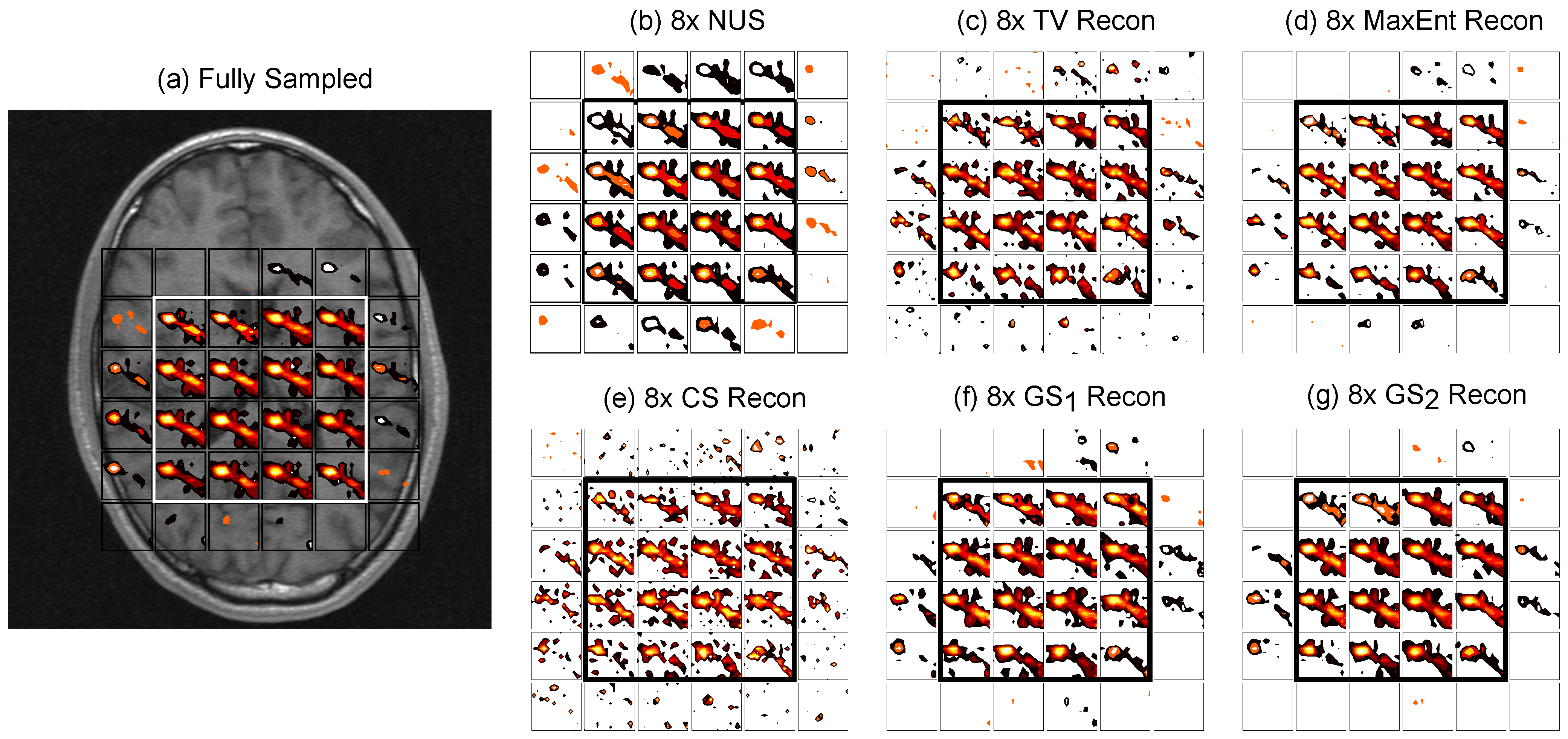
4.1. Gray Matter Brain Phantom
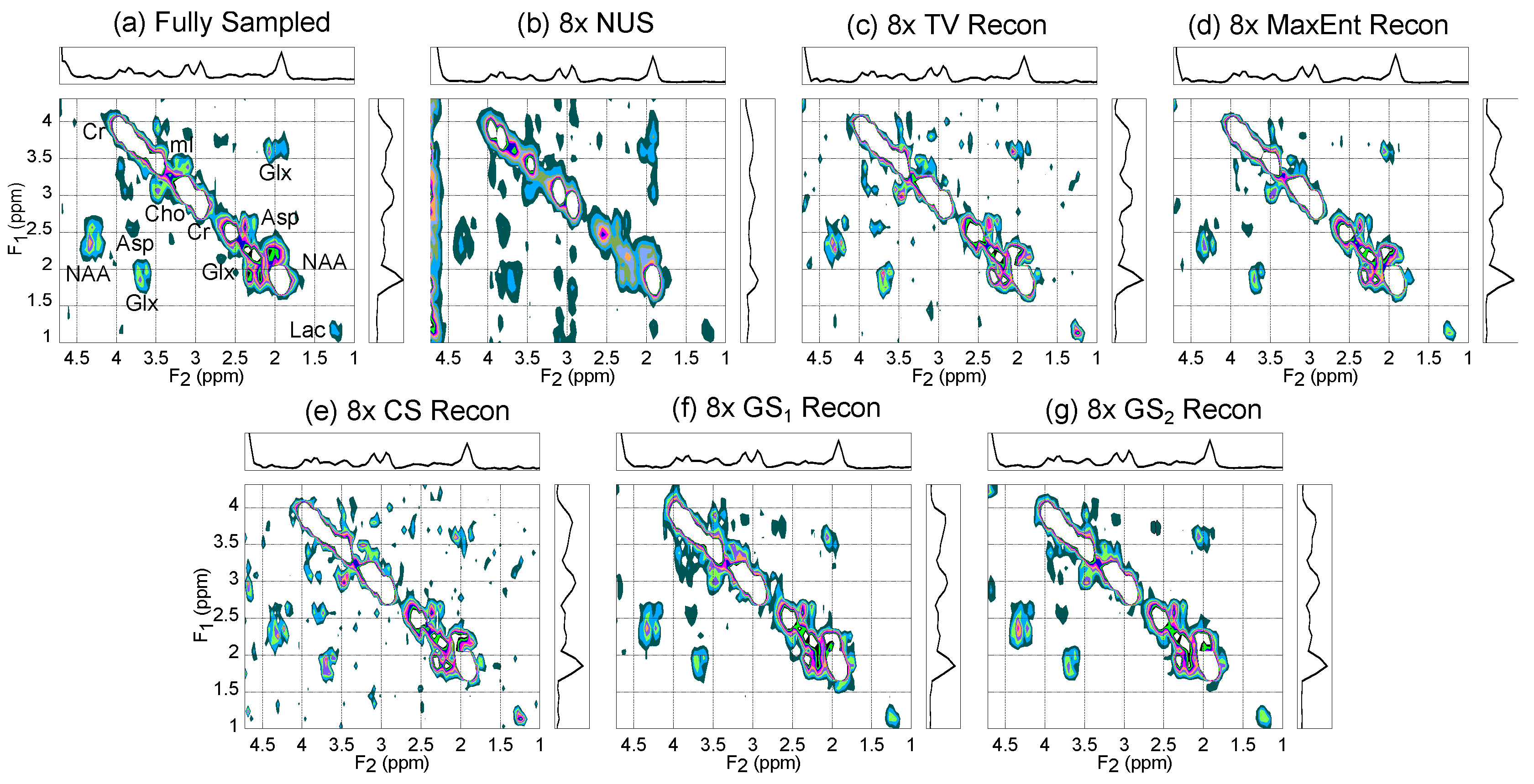
| (ppm) | (ppm) | |
|---|---|---|
| Diagonals: | ||
| Cho | 3.1–3.4 | 3.1–3.4 |
| Cr303 | 2.9–3.1 | 2.8–3.2 |
| Cr391 | 3.8–4.1 | 3.7–4.1 |
| Glx | 2.4–2.6 | 2.3–2.5 |
| Lac | 1.1–1.7 | 1.0–1.6 |
| mI | 3.5–3.8 | 3.4–3.7 |
| NAA | 1.7–2.3 | 1.7–2.1 |
| Cross Peaks: | ||
| Glx (Lower) | 1.7–2.2 | 3.4–4.1 |
| Glx (Upper) | 3.4–3.9 | 1.7–2.4 |
| NAA (Lower) | 2.0–3.0 | 4.0–4.5 |
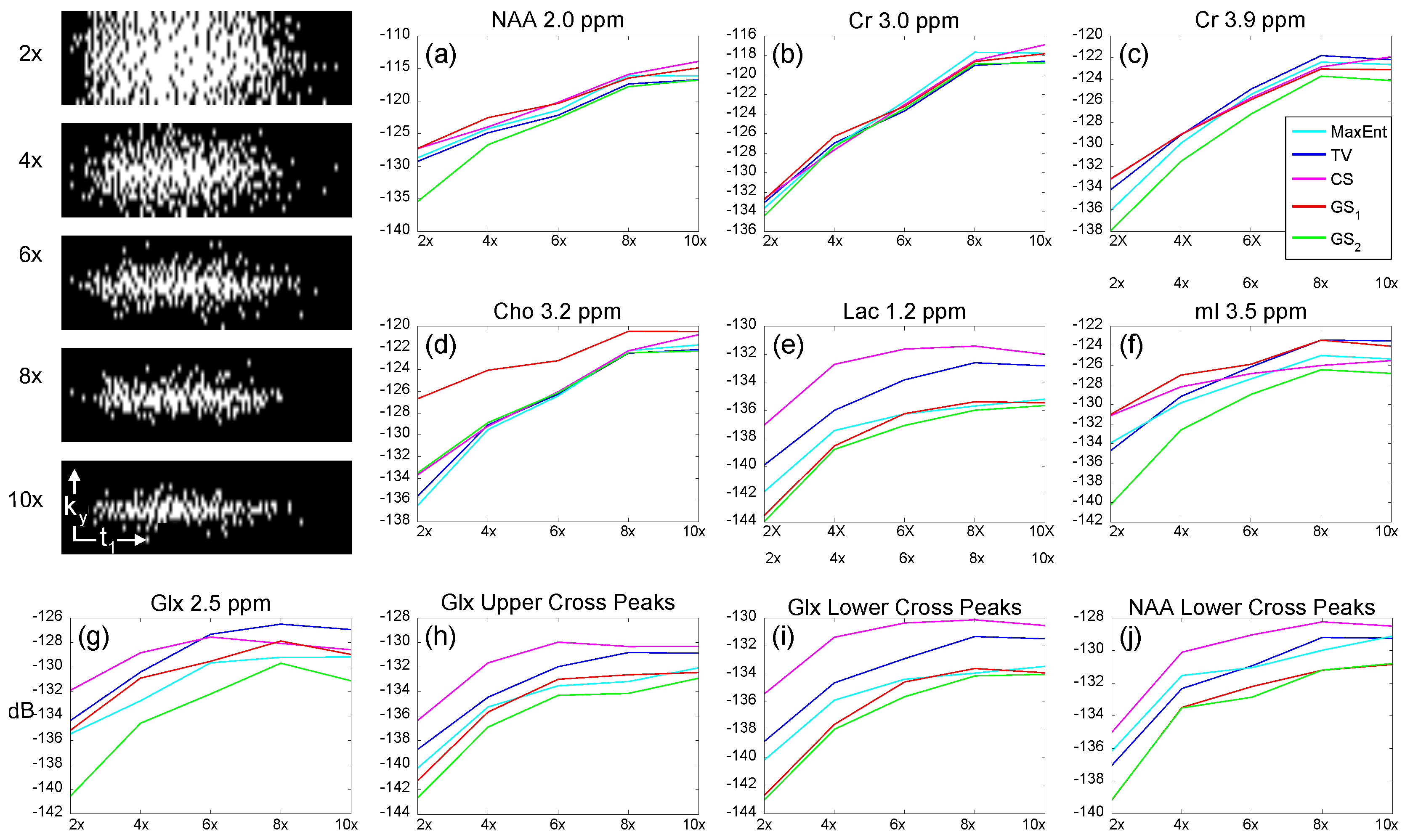
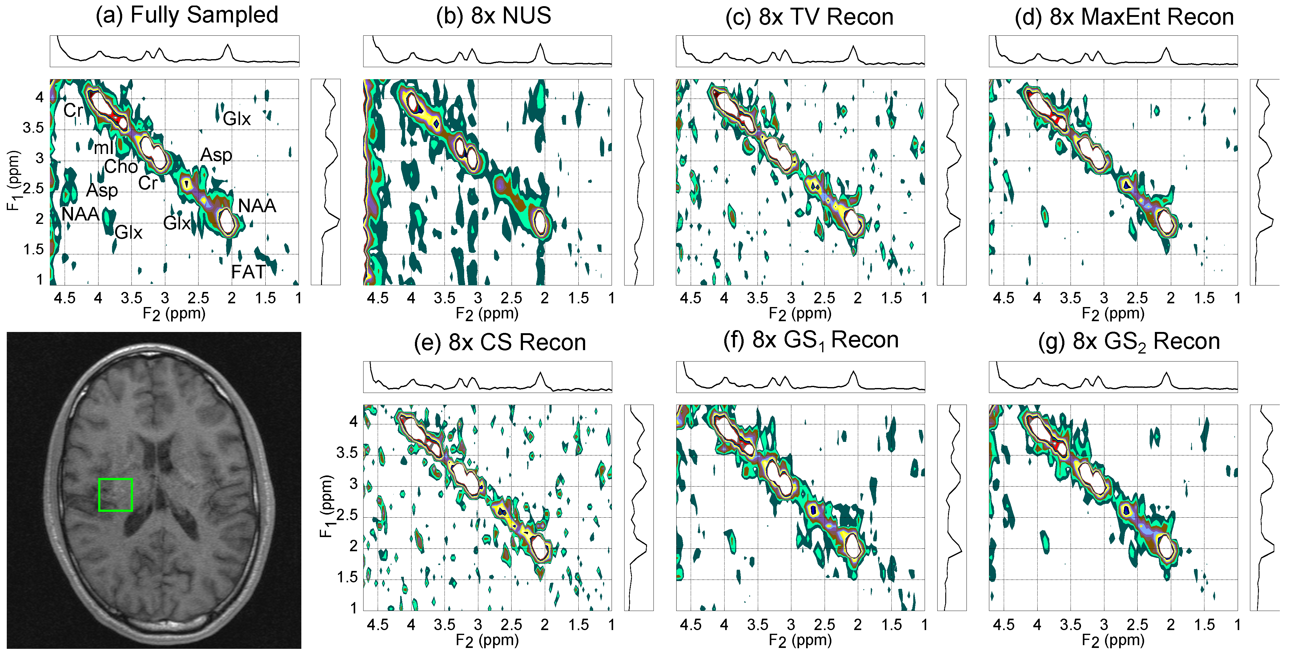
4.2. In Vivo Brain

| CS | TV | MaxEnt | GS | GS | |||||||||||||||
|---|---|---|---|---|---|---|---|---|---|---|---|---|---|---|---|---|---|---|---|
| 4× | 6× | 8× | 4× | 6× | 8× | 4× | 6× | 8× | 4× | 6× | 8× | 4× | 6× | 8× | |||||
| Lac 1.2 | −136.6 | −134.8 | −134.4 | −140.2 | −138.5 | −137.9 | −141.3 | −140.4 | −140.0 | −143.0 | −141.0 | −138.7 | −143.4 | −142.1 | −141.1 | ||||
| NAA 2.0 | −130.9 | −127.8 | −126.1 | −131.9 | −127.9 | −124.6 | −133.9 | −129.8 | −126.8 | −125.9 | −124.5 | −122.4 | −133.0 | −130.8 | −127.1 | ||||
| Glx 2.2 | −132.2 | −129.4 | −128.9 | −136.6 | −131.7 | −131.6 | −137.3 | −134.2 | −134.0 | −139.3 | −138.2 | −134.3 | −139.6 | −137.4 | −135.0 | ||||
| Cr 3.0 | −130.3 | −128.6 | −126.1 | −130.8 | −128.1 | −124.9 | −133.4 | −132.0 | −126.2 | −130.3 | −127.7 | −126.3 | −131.8 | −131.7 | −127.6 | ||||
| Cho 3.2 | −131.6 | −129.9 | −127.6 | −133.3 | −130.7 | −126.2 | −134.2 | −131.5 | −128.2 | −126.0 | −126.1 | −122.8 | −135.1 | −133.4 | −130.2 | ||||
| mI 3.5 | −129.1 | −128.5 | −128.1 | −132.0 | −130.9 | −127.3 | −131.3 | −131.5 | −129.0 | −131.3 | −131.2 | −128.8 | −138.2 | −136.3 | −133.3 | ||||
| Cr 3.9 | −131.0 | −130.0 | −128.2 | −132.6 | −129.4 | −126.6 | −134.3 | −131.8 | −129.5 | −137.5 | −133.5 | −132.5 | −136.6 | −134.4 | −130.1 | ||||
| Glx UCP | −136.3 | −134.9 | −133.6 | −140.7 | −139.2 | −136.4 | −144.6 | −142.0 | −141.4 | −146.0 | −142.6 | −137.9 | −146.1 | −143.1 | −141.6 | ||||
| Glx LCP | −135.5 | −134.8 | −133.7 | −139.7 | −138.1 | −137.2 | −142.2 | −139.7 | −138.3 | −143.1 | −139.5 | −138.3 | −144.5 | −141.7 | −139.9 | ||||
| NAA LCP | −134.3 | −132.9 | −132.5 | −137.8 | −136.0 | −135.2 | −139.2 | −137.8 | −136.1 | −140.3 | −137.2 | −134.5 | −141.4 | −139.4 | −136.9 | ||||
5. Discussion
6. Conclusions
Acknowledgments
Author Contributions
Conflicts of Interest
References
- Thomas, M.; Yue, K.; Binesh, N.; Davanzo, P.; Kumar, A.; Siegel, B.; Frye, M.; Curran, J.; Lufkin, R.; Martin, P.; et al. Localized Two-Dimensional Shift Correlated MR Spectroscopy of Human Brain. Magn. Reson. Med. 2001, 46, 58–67. [Google Scholar] [CrossRef] [PubMed]
- Ryner, L.; Sorenson, J.; Thomas, M. Localized 2D J-Resolved 1H MR spectroscopy: Strong coupling effects in vitro and in vivo. Magn. Reson. Imaging 1995, 13, 853–869. [Google Scholar] [CrossRef]
- Shulte, R.; Boesiger, P. ProFit: Two-Dimensional Prior-Knowledge Fitting of J-Resolved Spectra. NMR Biomed. 2006, 19, 255–263. [Google Scholar] [CrossRef] [PubMed]
- Negendank, W. Studies of Human Tumors by MRS: A Review. NMR Biomed. 1992, 5, 303–324. [Google Scholar] [CrossRef] [PubMed]
- Lipnick, S.; Verma, G.; Ramadan, S.; Furuyama, J.; Thomas, M.A. EP-COSI: Implementation and pilot evaluation in human calf in vivo. Magn. Reson. Med. 2010, 64, 947–956. [Google Scholar] [CrossRef] [PubMed]
- Mulkern, R.; Wong, S.; Winalski, C.; Jolesz, F. Contrast Manipulation and Artifact Assessment of 2D and 3D RARE Sequences. Magn. Reson. Imaging 1990, 8, 557–566. [Google Scholar] [CrossRef]
- Posse, S.; Tedeschi, G.; Risinger, R.; Ogg, R.; Le-Bihan, D. High Speed 1H Spectroscopic Imaging in Human Brain by Echo Planar Spatial-Spectral Encoding. Magn. Reson. Med. 1995, 33, 34–40. [Google Scholar] [CrossRef] [PubMed]
- Aue, W.; Bartholdi, E.; Ernst, R. Two-dimensional spectroscopy. Application to nuclear magnetic resonance. J. Chem. Phys. 1976, 64, 2229–2246. [Google Scholar] [CrossRef]
- Thomas, M.; Lipnick, S.; Velan, S.; Liu, X.; Banakar, S.; Binesh, N.; Ramadan, S.; Ambrosio, A.; Raylman, R.R.; Sayre, J.; et al. Investigation of breast cancer using two-dimensional MRS. NMR BioMed. 2008, 22, 77–91. [Google Scholar] [CrossRef] [PubMed]
- Donoho, D. Compressed Sensing. IEEE Trans. Inf. Theory 2006, 52, 1289–1306. [Google Scholar] [CrossRef]
- Candés, E.; Romberg, J.; Tao, T. Robust Uncertainty Principles: Exact Signal Reconstruction From Highly Incomplete Frequency Information. IEEE Trans. Inf. Theory 2006, 52, 489–509. [Google Scholar] [CrossRef]
- Lustig, M.; Donoho, D.; Pauly, J. Sparse MRI: The Application of Compressed Sensing for Rapid MR Imaging. Magn. Reson. Med. 2007, 58, 1182–1195. [Google Scholar] [CrossRef] [PubMed]
- Block, K.; Uecker, M.; Frahm, J. Undersampled Radial MRI with Multiple Coils. Iterative Image Reconstruction Using a Total Variation Constraint. Magn. Reson. Med. 2007, 57, 1086–1098. [Google Scholar] [CrossRef] [PubMed]
- Gamper, U.; Boesiger, P.; Kozerke, S. Compressed Sensing in Dynamic MRI. Magn. Reson. Med. 2008, 59, 365–373. [Google Scholar] [CrossRef] [PubMed]
- Hu, S.; Lustig, M.; Chen, A.; Crane, J.; Kerr, A.; Kelley, D.; Hurd, R.; Kurhanewicz, J.; Nelson, S.; Pauly, J.; et al. Compressed Sensing for Resolution Enhancement of Hyperpolarized 3C Flyback 3D-MRSI. J. Magn. Reson. 2008, 192, 258–264. [Google Scholar] [CrossRef] [PubMed]
- Furuyama, J.; Wilson, N.; Burns, B.; Nagarajan, R.; Margolis, D.; Thomas, M. Application of CS to Multidimensional Spectroscopic Imaging in Human Prostate. Magn. Reson. Med. 2012, 67, 1499–1505. [Google Scholar] [CrossRef] [PubMed]
- Burns, B.; Wilson, N.; Furuyama, J.; Thomas, M. Non-Uniformly Under-Sampled Multidimensional Spectroscopic Imaging in vivo: Maximum Entropy versus Compressed Sensing Reconstruction. NMR BioMed. 2013, 27, 191–201. [Google Scholar] [CrossRef]
- Yuan, M.; Lin, Y. Model selection and estimation in regression with grouped variables. Stat. Soc. B 2006, 68, 49–67. [Google Scholar] [CrossRef]
- Goldstein, T.; Osher, S. The Split Bregman Method for L1-Regularized Problems. SIAM J. Imaging Sci. 2009, 2, 323–343. [Google Scholar] [CrossRef]
- Zou, J.; Fu, Y.; Zhang, Q.; Li, H. Split Bregman algorithm for multiple measurement vector problem. Multidimens. Syst. Signal Process. 2013. [Google Scholar] [CrossRef]
- Usman, M.; Prieto, C.; Schaeffter, T.; Batchelor, P. k-t Group Sparse: A Method for Accelerating Dynamic MRI. Mag. Res. Med. 2011, 66, 1163–1176. [Google Scholar] [CrossRef] [PubMed]
- Prieto, C.; Usman, M.; Wild, J.; Kozerke, S.; Batchelor, P. Group Sparse Reconstruction Using Intensity-Based Clustering. Mag. Res. Med. 2013, 69, 1169–1179. [Google Scholar] [CrossRef] [PubMed]
- Rudin, L.; Osher, S.; Fatemi, E. Nonlienar Total Variation Based Noise Removal Algorithms. Physica D 1992, 60, 259–268. [Google Scholar] [CrossRef]
- Skilling, J.; Bryan, R. Maximum Entropy Image Reconstruction: General Algorithm. Mon. Not. R. Astr. Soc. 1984, 211, 111–124. [Google Scholar] [CrossRef]
- Donoho, D. For Most Large Underdetermined Systems of Linear Equations the Minimal ℓ1-norm Solution is Also the Sparsest Solution. Commun. Pure Appl. Math. 2006, 59, 797–829. [Google Scholar] [CrossRef]
- Daniell, G.; Hore, P. Maximum Entropy and NMR: A New Approach. J. Magn. Reson. 1989, 4, 515–536. [Google Scholar] [CrossRef]
- Friedman, B.R. Statistical Models for the Image Restoration Problem. Comput. Graph. Image Process. 1980, 12, 40–59. [Google Scholar] [CrossRef]
- Bertsekas, D. Multiplier Methods: A Survey. Automatica 1976, 12, 133–145. [Google Scholar] [CrossRef]
- Osher, S.; Burger, M.; Goldfarb, D.; Xu, J.; Yin, W. An iterative regularization method for total variation-based image restoration. Multiscale Model. Simul. 2005, 4, 460–489. [Google Scholar] [CrossRef]
- Huang, J.; Zhang, T. The Benefit of Group Sparsity. Ann. Stat. 2010, 38, 1978–2000. [Google Scholar] [CrossRef]
- Eldar, Y.; Mishali, M. Robust Recovery of Signals From a Structured Union of Subspaces. IEEE Trans. Inf. Theory 1980, 12, 5302–5316. [Google Scholar] [CrossRef]
- Eldar, Y.; Kuppinger, P.; Bölcskei, H. Block-Sparse Signals: Uncertainty Relations and Efficient Recovery. IEEE Trans. Signal Process. 2010, 58, 3042–3054. [Google Scholar] [CrossRef]
- Wei, D.; Yin, W.O.T.A.O.; Zhang, Y. Group Sparse Optimization by Alternating Direction Method; Technical Report; Dept. Comp. and App. Math., Rice University: Houston, Texas, USA, 2011. [Google Scholar]
- Chen, P.; Selesnick, I. Overlapping Group Shrinkage/Thresholding and Denoising; Technical Report; Polytechnic Institute of New York University: New York, NY, USA, 2012. [Google Scholar]
- Hoch, J.; Stern, A. NMR Data Processing; Wiley: New York, NY, USA, 1996. [Google Scholar]
© 2014 by the authors; licensee MDPI, Basel, Switzerland. This article is an open access article distributed under the terms and conditions of the Creative Commons Attribution license (http://creativecommons.org/licenses/by/3.0/).
Share and Cite
Burns, B.L.; Wilson, N.E.; Thomas, M.A. Group Sparse Reconstruction of Multi-Dimensional Spectroscopic Imaging in Human Brain in vivo. Algorithms 2014, 7, 276-294. https://doi.org/10.3390/a7030276
Burns BL, Wilson NE, Thomas MA. Group Sparse Reconstruction of Multi-Dimensional Spectroscopic Imaging in Human Brain in vivo. Algorithms. 2014; 7(3):276-294. https://doi.org/10.3390/a7030276
Chicago/Turabian StyleBurns, Brian L., Neil E. Wilson, and M. Albert Thomas. 2014. "Group Sparse Reconstruction of Multi-Dimensional Spectroscopic Imaging in Human Brain in vivo" Algorithms 7, no. 3: 276-294. https://doi.org/10.3390/a7030276
APA StyleBurns, B. L., Wilson, N. E., & Thomas, M. A. (2014). Group Sparse Reconstruction of Multi-Dimensional Spectroscopic Imaging in Human Brain in vivo. Algorithms, 7(3), 276-294. https://doi.org/10.3390/a7030276