Application of Imperialist Competitive Algorithm on Solving the Traveling Salesman Problem

Abstract

The imperialist competitive algorithm (ICA) is a new heuristic algorithm proposed for continuous optimization problems. The research about its application on solving the traveling salesman problem (TSP) is still very limited. Aiming to explore its ability on solving TSP, we present a discrete imperialist competitive algorithm in this paper. The proposed algorithm modifies the original rules of the assimilation and introduces the 2-opt algorithm into the revolution process. To examine its performance, we tested the proposed algorithm on 10 small-scale and 2 large-scale standard benchmark instances from the TSPLIB and compared the experimental results with that obtained by two other ICA-based algorithms and six other existing algorithms. The proposed algorithm shows excellent performance in the experiments and comparisons.

1. Introduction

Because of its widespread application and significant research value, the traveling salesman problem (TSP) has probably become the most classical, famous and extensively studied problem in the field of combinatorial optimization [1,2,3]. It can be simply described as to find out the shortest tour that starts from one city from the set of given cities, visits every given city once, and returns to the original finally. As a typical NP-hard combinatorial optimization problem, it is extremely difficult to solve [4]. Compared with the exact algorithms for solving TSP, the approximate algorithms are simpler. Although they cannot guarantee to find the optimal solution, often they can obtain a satisfactory solution. They are more suitable to be used to solve larger-scale TSP [5]. Many approximate algorithms have been applied to solve the TSP [6,7,8,9,10,11,12,13,14,15,16,17,18,19,20,21,22,23,24,25,26].

Imperialist competitive algorithm (ICA) is a new socio-politically motivated meta-heuristic algorithm proposed by Atashpaz-Gargari and Lucas in 2007, inspired by the colonial phenomenon in human society and history [27]. Although it has been successfully applied to many different optimization tasks and has shown great performance in both the convergence rate and the global optimal achievement [28,29,30,31,32,33], its application on solving TSP is still very limited. The literature [34] gives some results obtained by ICA, but the description about how to use ICA to solve TSP is ambiguous. The literature [35] submits a new approach, but in our test experiments, the approach cannot produce the results given in the literature. Mohammad Ahmadvand et al. [36] proposed a hybrid algorithm based on ICA and tabu search, using ICA to solve TSP at first and using a tabu search to improve the solution, however, the results obtained by the hybrid algorithm are not yet good enough.

Seeking to explore the potential of ICA and to find a novel and efficient way for solving TSP, we present a novel discrete ICA in this paper.

The rest of this paper is organized as follows. In Section 2, a brief introduction about the basic ICA is given. In Section 3, the proposed algorithm is set out in detail. In Section 4, the numerical experiments, results and related discussion are given. In Section 5, we conclude the paper and put forward the future works.

2. Basic Imperialist Competitive Algorithm

The ICA simulates the process of competition between empires in human society. It starts with a randomly generated initial population of size N, which are called countries, just like the chromosomes in the genetic algorithm. The cost of each country is calculated by the equation specific for the problem to be optimized. Then, countries are divided into imperialists and colonies. Imperialists are the best countries in the population, and colonies are the others left. Then the colonies are randomly distributed to the imperialists. The number of colonies that an imperialist obtains is proportional to its power. Here the power of each imperialist is calculated and normalized depended on its cost. The imperialist with bigger power value is better. One imperialist and its colonies consist of an empire together, thus several empires are initialized.

After, within each empire group, the colonies are moved to the position of the imperialist according to a certain rule. This process is called “assimilation”, simulates the assimilation process the imperialist implements on its colonies in a realistic society. Meanwhile, some colonies are randomly selected out and replaced with new randomly generated countries. This process is called “revolution”, just like the mutation in the genetic algorithm, simulates the sudden change in the socio-political characteristics of a colony in a realistic society. In the process of assimilation and revolution, if a colony becomes better than the imperialist, the colony and the imperialist will exchange their roles.

The competitive behavior between the empires is the core of the ICA. In this stage, all empires try to occupy colonies from others. Firstly, the total cost of every empire is calculated and normalized according to the formulas (1) and (2) [27], in where the T.C._n and the N.T.C._n stand for the total cost and the normalized total cost of the nth empire, respectively, and the ξ is a little positive number, whose value determines the role of the colonies in determining the total cost of the empire.

$$T.C{.}_n=Cost(imperialis{t}_n)+\xi ·mean\{Cost(colonies of empir{e}_n)\}$$

(1)

$$N.T.C{.}_n=T.C{.}_n-\underset{i}{\max }\{T.C{.}_i\}$$

(2)

Then, the weakest colony of the weakest empire is picked out. Other empires try to obtain it through competition. The success probability of each empire is given by the formula (3) [27] and form the vector P as the formula (4) [27]. A vector R with the same size as P whose elements are uniformly distributed random numbers is created as the formula (5) [27]. Then vector D is created by subtracting R from P, as the formula (6) [27]. The empire whose relevant index in D is maximized will obtain the mentioned colony at the end.

$${\mathrm{P}}_{P_n}=\left|\frac{N.T.C{.}_n}{{\displaystyle {\sum }_{i=1}^{N_{imp}}N.T.C{.}_i}}\right|$$

(3)

$$\mathrm{P}=[\hspace{0.17em}{p}_{P_1},p_{P_2},p_{P_3},\cdots ,p_{P_{N_{imp}}}]$$

(4)

$$\mathrm{R}=[\hspace{0.17em}{r}_1,r_2,r_3,\cdots ,r_{N_{imp}}], \mathrm{w}\mathrm{h}\mathrm{e}\mathrm{r}\mathrm{e} r_i\sim U(0,1) \mathrm{a}\mathrm{n}\mathrm{d} 1 \le i\le N_{imp}$$

(5)

$$\mathrm{D}=\mathrm{P}-\mathrm{R}=[\hspace{0.17em}{D}_1,D_2,D_3,\cdots ,D_{N_{imp}}]=[\hspace{0.17em}{p}_{P_1}-r_1,p_{P_2}-r_2,p_{P_3}-r_3,\cdots ,p_{P_{N_{imp}}}-r_{N_{imp}}]$$

(6)

There is just one empire left or a preset maximum number of iterations is reached is usually utilized as the termination condition of the algorithm. The competition proceeds until the termination condition is met. The weak empire gradually loses its colonies and the mighty empire occupies more and more colonies. The empire loses all its colonies will be collapsed. The final residual imperialist stands for the solution.

The pseudo code of the basic ICA is shown in Figure 1.

Figure 1. The pseudo code of the basic imperialist competitive algorithm (ICA).

Figure 1. The pseudo code of the basic imperialist competitive algorithm (ICA).

3. Approach to Discretize the ICA for TSP

Since the basic ICA is proposed for numerical function optimization, when it is utilized to solve TSP, some detail rules in the algorithm should be modified.

3.1. Generate Initial Population and Initiate Empires

The discrete ICA we propose starts with a randomly generated initial population of size N also. The only difference is that here a country represents a tour. We use a randomly arranged integer sequence to represent a country. There are n integers from 1 to n in the sequence, each integer represents a city, appears only once and the order of them represents the order of the visited cities. For example, in a 4-cities-TSP, the sequence (1, 4, 3, 2) implies that the tour starts from the city 1 to city 4, then goes from city 4 to city 3, then goes to city 2, finally returning from city 2 to city 1. The cost of a country is the total length of the tour it represents. Because of the aim is to find out the shortest tour, a country which represents a shorter tour is better, so the power of a country can be directly defined as the reciprocal of its cost.

At the process of forming initial empires, we are required to assign the colonies to the imperialists. here we define that this assignment is according to the formula (7), in where the N denotes the size of the initial population, the m denotes the number of imperialists, N and m can be set freely according to the size of the TSP to be solved, the k_j denotes the number of colonies assigned to the jth imperialist and the f_j denotes the cost of the jth imperialist.

$$\begin{array}{ll}{k}_j=\mathrm{int}\left(\frac{1/f_j}{{\displaystyle {\sum }_{j=1}^m(1/f_j)}}(N-m)\right)\hfill & j=1,2,\mathrm{...}m-1\hfill \\ k_m=N-m-{\displaystyle {\sum }_{i=1}^{m-1}{k}_i}\hfill & j=m\hfill \end{array}$$

(7)

3.2. The Modified Assimilation Process

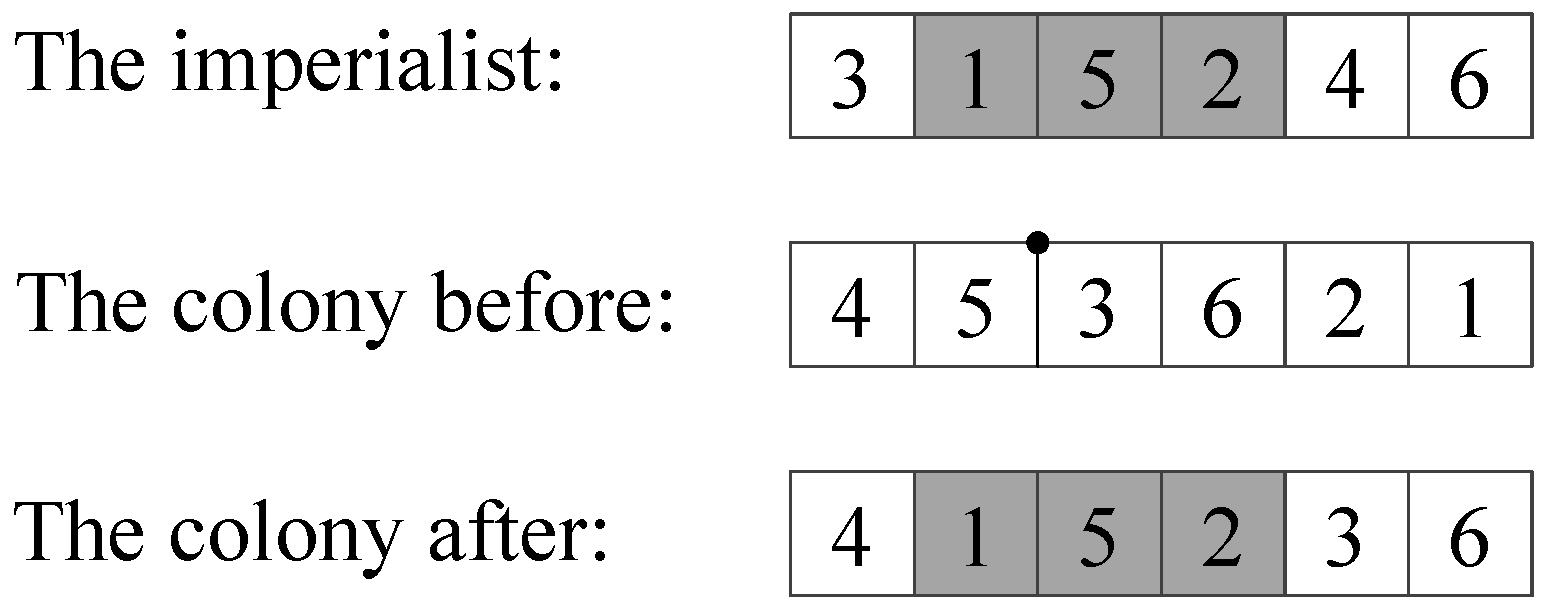
In the assimilation process, colonies obtain information from and adjust themselves to keep consistent with the relevant imperialist. This process can be viewed as a learning process of the colonies from the imperialist. Basing on the country encoding method, we redefine the detail rule of the assimilation process as follows: A subsequence is randomly chosen from the relevant imperialist, and a position is randomly chosen from the colony. Then, the mentioned subsequence is inserted to the mentioned position. Finally, the cities which are included in the subsequence are deleted from the part coming from the previous colony. This process is shown by Figure 2, in where the tour (3, 1, 5, 2, 4, 6) is a hypothetical tour just used as an example. The subsequence (1 5 2) is chosen from the imperialist and the position between city 5 and city 3 is chosen from the colony. The subsequence (1 5 2) which may include effective information, is transferred from the imperialist to its colony after the assimilation process.

Figure 2. An example of the redefined assimilation.

Figure 2. An example of the redefined assimilation.

3.3. The Modified Revolution Process

Obviously, we can achieve the revolution process by replacing the randomly selected colonies with an equal number of new randomly generated countries, like the method in the basic ICA. However, here, in order to enhance the ability of the proposed algorithm further, we introduce the 2-opt algorithm [37] into the revolution process.

Due to its simplicity and effectiveness, the 2-opt algorithm is probably the most widely used local search approach for solving TSP. It can be applied to an arbitrary initial tour, and searches the shortest tour by changing the visiting order of cities, but the 2-opt algorithm often takes a very long time, especially when it is applied in a larger number of candidate tours.

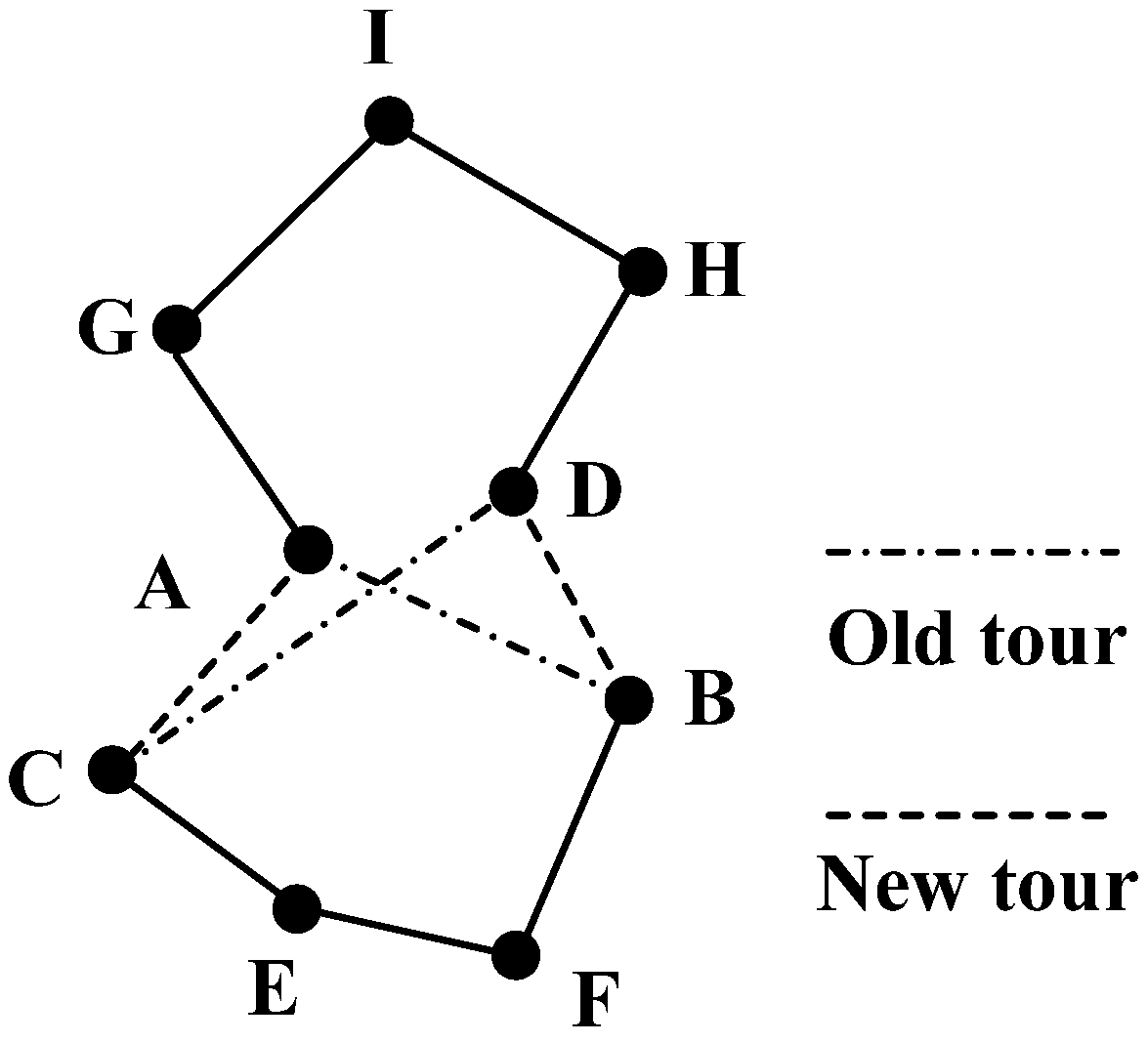
Figure 3 shows an illustration of the 2-opt algorithm. Here, the tour (A-B-F-E-C-D-H-I-G-A) presents an example tour before using 2-opt algorithm. Firstly, the length of this tour is calculated. Then a link A-B and another link C-D are selected out. A new tour is generated by linking A and C, B and D, respectively. If the new tour (A-C-E-F-B-D-H-I-G-A) is shorter than the old tour, then, the new tour is accepted. The above procedure is replicated for all links between each two cities until there is no more decrease of the total tour length.

Figure 3. An illustration of the 2-opt algorithm.

Figure 3. An illustration of the 2-opt algorithm.

Our way goes as follows: for every empire, take out a part of colonies randomly from its colonies, apply the 2-opt algorithm to them, and replace them with the improved. Because the revolution process is applied to a few countries, introducing the 2-opt algorithm into it will not take a very long time.

The pseudo code of the proposed algorithm is shown in Figure 4. It is similar to the pseudo code of the basic ICA, but is different on the specific operations of the step 1, step 2 and step 3.

Figure 4. The pseudo code of the proposed algorithm.

Figure 4. The pseudo code of the proposed algorithm.

4. Numerical Experiments, Results and Discussions

4.1. Experiments Settings

In order to verify its effectiveness, we test the proposed algorithm on 12 standard benchmark instances (listed in the Table 1) from the TSPLIB [38]. The first 10 instances are small-scale problems, with sizes ranging from 51 to 150 cities, and the last two are large-scale problems, whose size is 1323 and 1400 respectively. To avoid the effects caused by the randomness of the algorithm, the experiments for the former eight instances are repeated 20 times independently, the experiments for KroA150 and KroB150 are repeated 10 times independently, and the experiments for the last two instances are repeated 5 times independently, considering the consumption of time. As the calculation method of the TSPLIB, the distance between two cities is computed using Euclidean distance equation and rounded to an integer.

Table 1. The parameters set for every instance.

Instance	Num.C	Num.E	Num.Ite	Instance	Num.C	Num.E	Num.Ite
eil51	100	6	200	berlin52	100	6	200
st70	100	6	200	eil76	100	6	200
pr76	100	6	200	kroA100	100	6	200
kroB100	100	6	200	eil101	100	6	300
kroA150	150	6	300	kroB150	150	8	350
rl1323	200	10	400	fl1400	200	10	400

Table 1. The parameters set for every instance.

Instance	Num.C	Num.E	Num.Ite	Instance	Num.C	Num.E	Num.Ite
eil51	100	6	200	berlin52	100	6	200
st70	100	6	200	eil76	100	6	200
pr76	100	6	200	kroA100	100	6	200
kroB100	100	6	200	eil101	100	6	300
kroA150	150	6	300	kroB150	150	8	350
rl1323	200	10	400	fl1400	200	10	400

The proposed algorithm is coded in MATLAB R2010b. All the experiments are finished on a PC with Core 2 Duo at 2.2 GHZ, 2 GB RAM and Windows Vista Home Basic Operating system. In our tests, the revolution rate is set to 0.3 and the ξ is set to 0.1. We specify a maximum number of iterations for each test. The algorithm stopped after getting to the iterations number. The number of initial countries, initial empires and iterations set for every instance are shown in Table 1, represented by “Num.C”, “Num.E” and “Num.Ite” respectively. Larger scale TSP means higher solving difficulty, so we set more population size, more empire numbers and more iterations numbers for the larger scale TSP. Note that the parameters we listed here may be not the best. Actually, in our previous experiments, we found that the proposed algorithm is not very sensitive to the initial parameters.

In order to examine the role of 2-opt algorithm in the proposed algorithm (abbreviated as DICA1 in the following), another discrete ICA (abbreviated as DICA2 in the following) is also tested on the mentioned instances for making a comparison. In the DICA2, the assimilation process is the same as that in the DICA1, but the revolution process is achieved by replacing the randomly selected colonies with an equal number of new randomly generated countries. For fairness, the parameters set in the DICA2 are same as those in the DICA1.

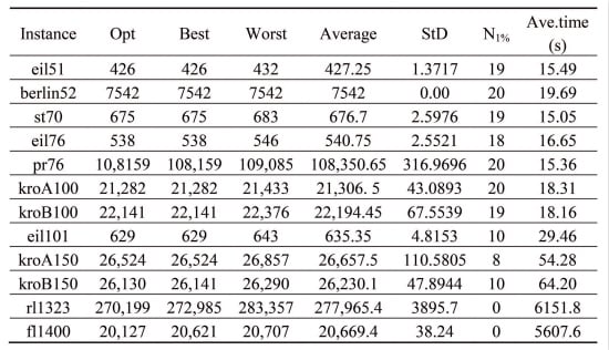
Table 2 shows the experimental results. The column “opt” represents the length of the known optimal solution of every instance. The columns “Best”, “Worst”, “Ave” and “StD” represent the best, the worst found result, the average and the stand deviation of the results for every instance, respectively. The column “N_1%” denotes the number of the found results that are within 1% deviation of the optimality over the experiments for every instance. The last column “Ave.time” represents the average running time for every instance. The bold data in the table are better.

Table 2. The results of the experiments.

Instance	Opt	Algorithm	Best	Worst	Average	StD	N1%	Ave.time (s)
eil51	426	DICA1	426	432	427.25	1.3717	19	15.49
		DICA2	590	770	700.6	43.9167	0	14.77
berlin52	7542	DICA1	7542	7542	7542	0.00	20	19.69
		DICA2	11,034	14,074	12,229.55	736.6680	0	16.87
st70	675	DICA1	675	683	676.7	2.5976	19	15.05
		DICA2	1300	1702	1518.2	93.2386	0	14.54
eil76	538	DICA1	538	546	540.75	2.5521	18	16.65
		DICA2	972	1298	1180	70.0669	0	15.86
pr76	10,8159	DICA1	108,159	109,085	108,350.65	316.9696	20	15.36
		DICA2	228,851	280,746	258,438.5	1333.2	0	15.12
kroA100	21,282	DICA1	21,282	21,433	21,306. 5	43.0893	20	18.31
		DICA2	66,573	84,480	73,032.3	4561.7	0	18.28
kroB100	22,141	DICA1	22,141	22,376	22,194.45	67.5539	19	18.16
		DICA2	65,905	88,172	73,587.9	5113.6	0	17.98
eil101	629	DICA1	629	643	635.35	4.8153	10	29.46
		DICA2	1426	1751	1574.3	82.1956	0	25.49
kroA150	26,524	DICA1	26,524	26,857	26,657.5	110.5805	8	54.28
		DICA2	102,953	118,004	109, 867.7	4397.2	0	44.67
kroB150	26,130	DICA1	26,141	26,290	26,230.1	47.8944	10	64.20
		DICA2	97,697	109,665	105,396.8	4432.1	0	53.17
rl1323	270,199	DICA1	272,985	283,357	277,965.4	3895.7	0	6151.8
		DICA2	7,311,486	7,491,391	7,398,724.4	74,062	0	179.71
fl1400	20,127	DICA1	20,621	20,707	20,669.4	38.24	0	5607.6
		DICA2	1,196,412	1,226,156	1,208,172.6	13,065	0	184.39

Table 2. The results of the experiments.

Instance	Opt	Algorithm	Best	Worst	Average	StD	N1%	Ave.time (s)
eil51	426	DICA1	426	432	427.25	1.3717	19	15.49
		DICA2	590	770	700.6	43.9167	0	14.77
berlin52	7542	DICA1	7542	7542	7542	0.00	20	19.69
		DICA2	11,034	14,074	12,229.55	736.6680	0	16.87
st70	675	DICA1	675	683	676.7	2.5976	19	15.05
		DICA2	1300	1702	1518.2	93.2386	0	14.54
eil76	538	DICA1	538	546	540.75	2.5521	18	16.65
		DICA2	972	1298	1180	70.0669	0	15.86
pr76	10,8159	DICA1	108,159	109,085	108,350.65	316.9696	20	15.36
		DICA2	228,851	280,746	258,438.5	1333.2	0	15.12
kroA100	21,282	DICA1	21,282	21,433	21,306. 5	43.0893	20	18.31
		DICA2	66,573	84,480	73,032.3	4561.7	0	18.28
kroB100	22,141	DICA1	22,141	22,376	22,194.45	67.5539	19	18.16
		DICA2	65,905	88,172	73,587.9	5113.6	0	17.98
eil101	629	DICA1	629	643	635.35	4.8153	10	29.46
		DICA2	1426	1751	1574.3	82.1956	0	25.49
kroA150	26,524	DICA1	26,524	26,857	26,657.5	110.5805	8	54.28
		DICA2	102,953	118,004	109, 867.7	4397.2	0	44.67
kroB150	26,130	DICA1	26,141	26,290	26,230.1	47.8944	10	64.20
		DICA2	97,697	109,665	105,396.8	4432.1	0	53.17
rl1323	270,199	DICA1	272,985	283,357	277,965.4	3895.7	0	6151.8
		DICA2	7,311,486	7,491,391	7,398,724.4	74,062	0	179.71
fl1400	20,127	DICA1	20,621	20,707	20,669.4	38.24	0	5607.6
		DICA2	1,196,412	1,226,156	1,208,172.6	13,065	0	184.39

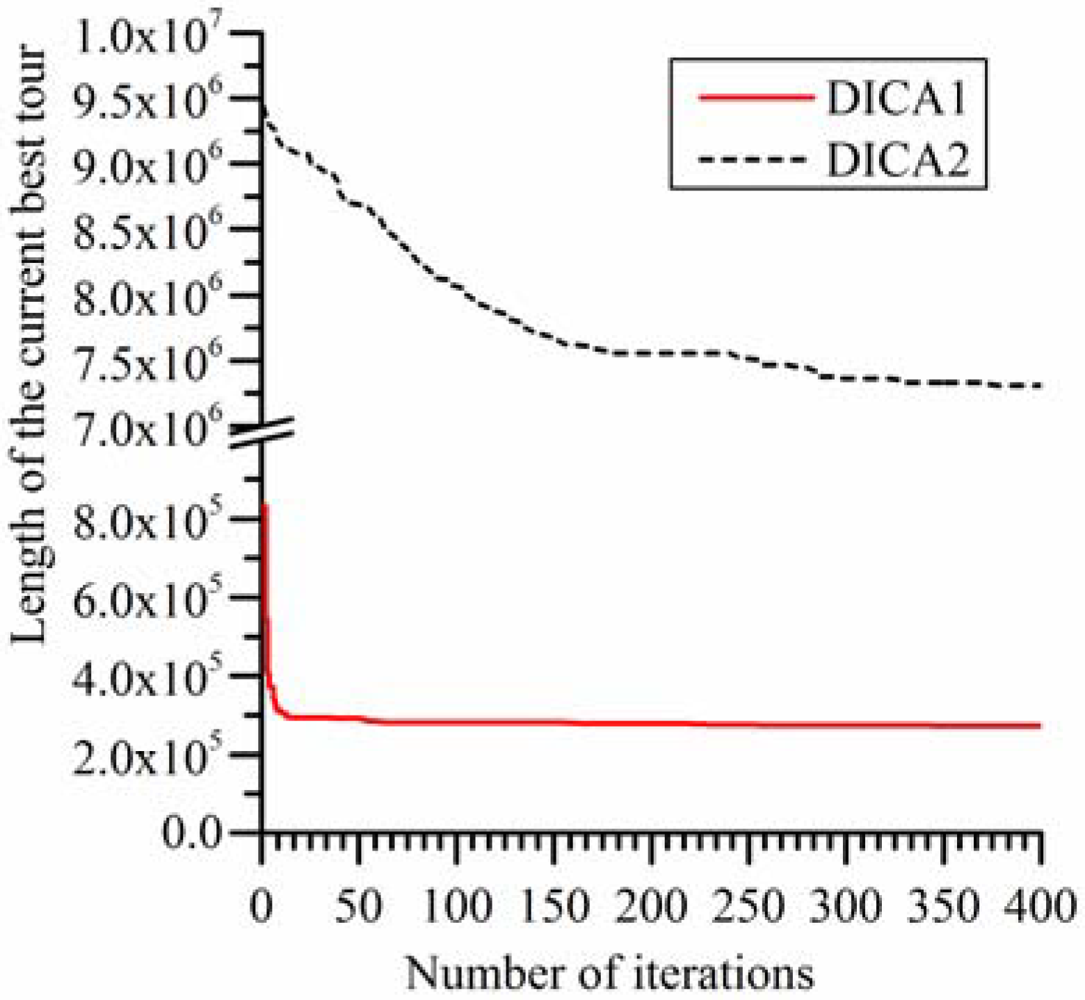
Figure 5. Trend lines of the two algorithms on rl1323.

Figure 5. Trend lines of the two algorithms on rl1323.

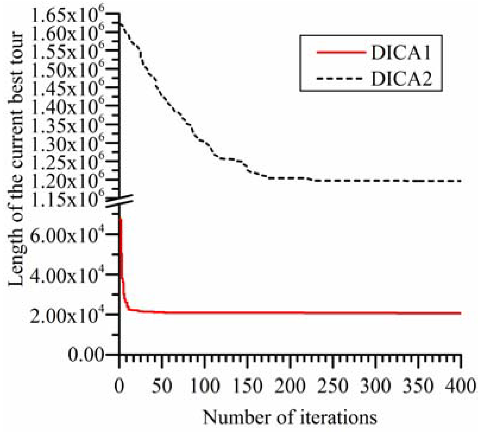
Figure 5 and Figure 6 show the trend lines of the DICA1 and the DICA2 on rl1323 and fl1400. They are utilized to compare the convergence process of the two algorithms. Limited by the length of the article, the trend lines of the two algorithms on other instances are not given here. Figure 5 and Figure 6 are utilized as a representative.

Figure 6. Trend lines of the two algorithms on fl1400.

Figure 6. Trend lines of the two algorithms on fl1400.

4.2. Discussions of the Results Obtained by the Proposed Algorithm

It can be seen from Table 2, for the former nine instances, the proposed algorithm (DICA1) found the known optimal solution, and for last three instances, though the known optimal solutions are not found, the best result found by the proposed algorithm are very close to the known optimal solutions. Their deviations with the corresponding known optimal solution are only 0.0421%, 1.0311% and 2.4544%, respectively. The average of the results for every instance is also quite close to the known optimal solution. Only for eil101, pr1323 and fl1400, the deviation with the known optimal solution exceeds 1%. For all the former ten instances except eil101, the probability of finding a solution which is within 1% deviation with the known optimal solution can reach more than 80%, especially, for berlin52, pr76, kroA100 and kroB150, it reaches 100%. In addition, for berlin52, the proposed algorithm found the known optimal solution in every test.

4.3. Discussions of the Role of 2-opt Algorithm

From Table 2, Figure 5 and Figure 6, it can be seen that, compared with the DICA1, the convergence rate of the DICA2 is slower, and the results it obtained are also worse. In the earlier stage of iterations, the convergence rate of the DICA2 is acceptable, but in the later stage of iterations, it stagnated at a solution which is very poor. The cause of this phenomenon is that in the earlier stage of the iterations, the individuals in the population are diverse and generally bad, it is very easy to find a solution which is better than the current best solution in the assimilation process, in the revolution process and in the competition process; but with the increase of the number of iterations, all the individuals in the population become more and more similar with the imperialist, the diversity of population decline, relying on the revolution process which using randomly generated countries to obtain a solution which is better than the current best solution is very difficult, so the DICA2 very easily stagnates at a very poor solution.

In DICA1, the revolution process is achieved by improved some randomly selected colonies by the 2-opt algorithm. Due to its strong local search ability, the 2-opt algorithm can greatly improve the quality of a colony, using this mechanism can easily find a solution which is greatly better than the current best solution. Meanwhile, the mechanism of the DICA1 can quickly replace the new find best solution to the position of the imperialist, and then to guide the further evolution of the entire population. So its convergence rate is very fast and the solutions it obtained are very good.

The revised assimilation makes it possible that utilizing the original ICA to solve TSP, and the revised revolution combined with 2-opt algorithm ensures the algorithm to find a superior solution quickly.

Furthermore, it can be seen from the last column “Ave.time”, when the scale of TSP is small, using 2-opt algorithm would not significantly increase the time consumption. When the scale of TSP is large, the time consumption increases obviously. The main reason is that the 2-opt algorithm costs more time when applied to solve large-scale TSP.

4.4. Compared with Other Two ICA-Based Algorithms

The results obtained by the DICA1 are compared with that obtained by other two ICA-based algorithms for solving TSP. One is proposed in literature [34] (abbreviated as OICA in the following) and another is proposed in literature [36], combined with tabu search (abbreviated as ICATS in the following). The comparison is arranged in Table 3, in where the column “Best.Err” and “Ave.Err” represent the percentage deviation of the best result and the average of the results over the known optimal solution, respectively, calculated as the formula 8, the “NA” represents that the data is not given in the corresponding literature. The bold data in the table are best.

$$Err=(the result-opt)/opt\hspace{0.17em}\times \hspace{0.17em}100\%$$

(8)

Table 3. Compared with two other ICA-based algorithms.

Instance	DICA1		ICATS		OICA
	Best.Err (%)	Ave.Err (%)	Best.Err (%)	Ave.Err (%)	Best.Err (%)	Ave.Err (%)
eil51	0	0.2934	0	2.5822	1.39	NA
berlin52	0	0	NA	NA	0.09	NA
st70	0	0.2519	NA	NA	0.44	NA
eil76	0	0.5112	NA	NA	0.99	NA
pr76	0	0.1771	0	0.1072	NA	NA
kroA100	0	0.1151	0	0.5451	0.10	NA
kroB100	0	0.2414	0	0.8356	0.38	NA
eil101	0	1.01	0	7.9491	NA	NA
kroA150	0	0.5033	0	0.7917	NA	NA

Table 3. Compared with two other ICA-based algorithms.

Instance	DICA1		ICATS		OICA
	Best.Err (%)	Ave.Err (%)	Best.Err (%)	Ave.Err (%)	Best.Err (%)	Ave.Err (%)
eil51	0	0.2934	0	2.5822	1.39	NA
berlin52	0	0	NA	NA	0.09	NA
st70	0	0.2519	NA	NA	0.44	NA
eil76	0	0.5112	NA	NA	0.99	NA
pr76	0	0.1771	0	0.1072	NA	NA
kroA100	0	0.1151	0	0.5451	0.10	NA
kroB100	0	0.2414	0	0.8356	0.38	NA
eil101	0	1.01	0	7.9491	NA	NA
kroA150	0	0.5033	0	0.7917	NA	NA

From Table 3, it can be seen that the performance of the OICA is the worst in the three algorithms. On every instance, it cannot obtain the known optimal solution. The performance of the ICATS is centered in the three algorithms, though it can obtain the known optimal solution for every instance, but the average of the results obtained by it for every instance except pr76 is worse than that obtained by the DICA1. The performance of the DICA1 is the best in the three algorithms.

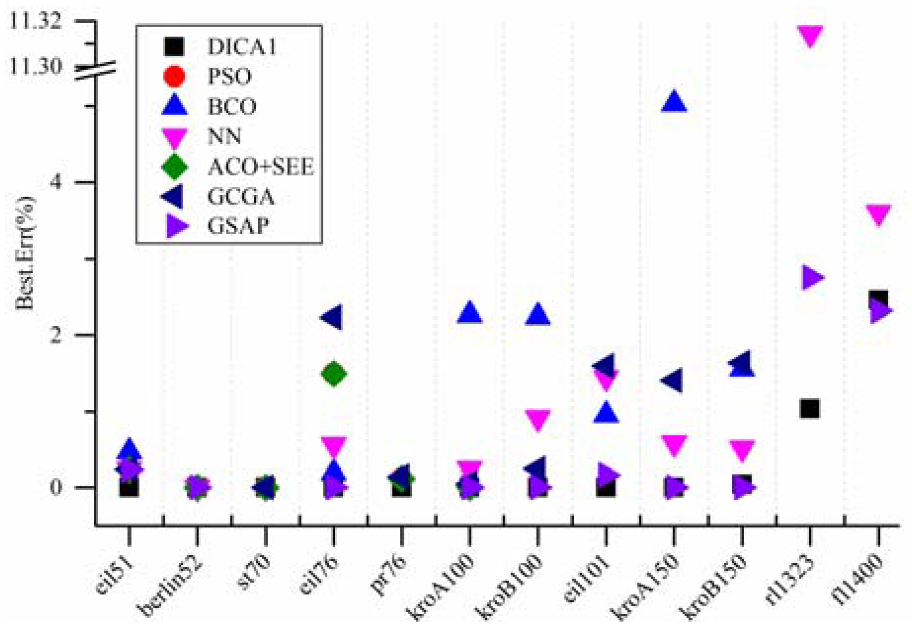
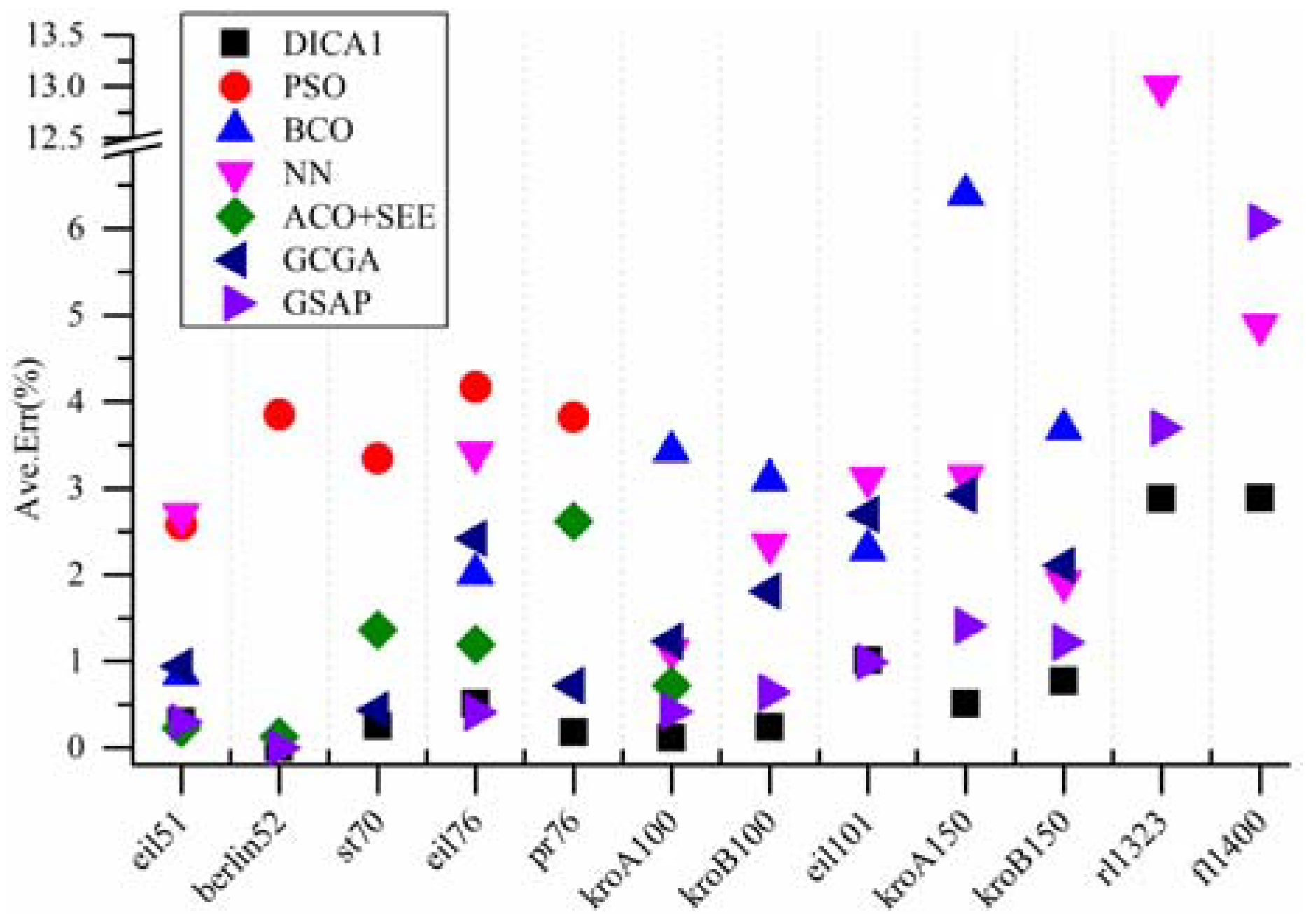
4.5. Compared with Other Six Heuristic Algorithms

Meanwhile, the results are compared with that obtained by the particle swarm optimization (PSO) [19], the bee colony optimization (BCO) [6], the self-organizing Neural Network (NN) [20], the improved ACO with Pheromone Correction Strategy (ACO+SEE) [14], the generalized chromosome genetic algorithm (GCGA) [25] and the genetic simulated annealing ant colony system with particle swarm optimization techniques (GSAP) [22], shown in Table 4 and Table 5. The meanings of the fields in Table 4 and Table 5 are same as those in Table 3. More intuitive comparisons are shown in Figure 7 and Figure 8.

Table 4. Compared with the particle swarm optimization (PSO), the bee colony optimization (BCO) and the Neural Network (NN).

Instance	DICA1		PSO		BCO		NN
	Best.Err (%)	Ave.Err (%)	Best.Err (%)	Ave.Err (%)	Best.Err (%)	Ave.Err (%)	Best.Err (%)	Ave.Err (%)
eil51	0	0.2934	0.2347	2.5751	0.4695	0.85	0.2347	2.6925
berlin52	0	0	0	3.8458	NA	NA	0	5.1777
st70	0	0.2519	0	3.3422	NA	NA	NA	NA
eil76	0	0.5112	1.487	4.1673	0.1859	2.01	0.5576	3.4071
pr76	0	0.1771	0.1119	3.8176	NA	NA	NA	NA
kroA100	0	0.1151	NA	NA	2.2601	3.43	0.2396	1.1311
kroB100	0	0.2414	NA	NA	2.2402	3.1	0.9123	2.3507
eil101	0	1.01	NA	NA	0.9539	2.29	1.4308	3.1208
kroA150	0	0.5033	NA	NA	5.0294	6.39	0.5806	3.1367
kroB150	0.0421	0.7658	NA	NA	1.55	3.68	0.5128	1.9207
rl1323	1.0311	2.8743	NA	NA	NA	NA	11.3143	12.9961
fl1400	2.4544	2.8817	NA	NA	NA	NA	3.5972	4.8840

Table 4. Compared with the particle swarm optimization (PSO), the bee colony optimization (BCO) and the Neural Network (NN).

Instance	DICA1		PSO		BCO		NN
	Best.Err (%)	Ave.Err (%)	Best.Err (%)	Ave.Err (%)	Best.Err (%)	Ave.Err (%)	Best.Err (%)	Ave.Err (%)
eil51	0	0.2934	0.2347	2.5751	0.4695	0.85	0.2347	2.6925
berlin52	0	0	0	3.8458	NA	NA	0	5.1777
st70	0	0.2519	0	3.3422	NA	NA	NA	NA
eil76	0	0.5112	1.487	4.1673	0.1859	2.01	0.5576	3.4071
pr76	0	0.1771	0.1119	3.8176	NA	NA	NA	NA
kroA100	0	0.1151	NA	NA	2.2601	3.43	0.2396	1.1311
kroB100	0	0.2414	NA	NA	2.2402	3.1	0.9123	2.3507
eil101	0	1.01	NA	NA	0.9539	2.29	1.4308	3.1208
kroA150	0	0.5033	NA	NA	5.0294	6.39	0.5806	3.1367
kroB150	0.0421	0.7658	NA	NA	1.55	3.68	0.5128	1.9207
rl1323	1.0311	2.8743	NA	NA	NA	NA	11.3143	12.9961
fl1400	2.4544	2.8817	NA	NA	NA	NA	3.5972	4.8840

Table 5. Compared with the improved ACO with Pheromone Correction Strategy (ACO + SEE), the generalized chromosome genetic algorithm (GCGA) and the genetic simulated annealing ant colony system with particle swarm optimization techniques (GSAP).

Instance	DICA1		ACO + SEE		GCGA		GSAP
	Best.Err (%)	Ave.Err (%)	Best.Err (%)	Ave.Err (%)	Best.Err (%)	Ave.Err (%)	Best.Err (%)	Ave.Err (%)
eil51	0	0.2934	0.2347	0.23	0.2347	0.94	0.23	0.3
berlin52	0	0	0	0.13	NA	NA	0	0
st70	0	0.2519	0	1.36	0	0.44	NA	NA
eil76	0	0.5112	1.487	1.19	2.2305	2.42	0	0.41
pr76	0	0.1771	0.1119	2.62	0.1378	0.72	NA	NA
kroA100	0	0.1151	0	0.72	0.047	1.23	0	0.42
kroB100	0	0.2414	NA	NA	0.2439	1.81	0	0.64
eil101	0	1.01	NA	NA	1.5898	2.7	0.16	0.99
kroA150	0	0.5033	NA	NA	1.3987	2.92	0	1.41
kroB150	0.0421	0.7658	NA	NA	1.6303	2.11	0	1.22
rl1323	1.0311	2.8743	NA	NA	NA	NA	2.7546	3.6945
fl1400	2.4544	2.8817	NA	NA	NA	NA	2.3153	6.0746

Table 5. Compared with the improved ACO with Pheromone Correction Strategy (ACO + SEE), the generalized chromosome genetic algorithm (GCGA) and the genetic simulated annealing ant colony system with particle swarm optimization techniques (GSAP).

Instance	DICA1		ACO + SEE		GCGA		GSAP
	Best.Err (%)	Ave.Err (%)	Best.Err (%)	Ave.Err (%)	Best.Err (%)	Ave.Err (%)	Best.Err (%)	Ave.Err (%)
eil51	0	0.2934	0.2347	0.23	0.2347	0.94	0.23	0.3
berlin52	0	0	0	0.13	NA	NA	0	0
st70	0	0.2519	0	1.36	0	0.44	NA	NA
eil76	0	0.5112	1.487	1.19	2.2305	2.42	0	0.41
pr76	0	0.1771	0.1119	2.62	0.1378	0.72	NA	NA
kroA100	0	0.1151	0	0.72	0.047	1.23	0	0.42
kroB100	0	0.2414	NA	NA	0.2439	1.81	0	0.64
eil101	0	1.01	NA	NA	1.5898	2.7	0.16	0.99
kroA150	0	0.5033	NA	NA	1.3987	2.92	0	1.41
kroB150	0.0421	0.7658	NA	NA	1.6303	2.11	0	1.22
rl1323	1.0311	2.8743	NA	NA	NA	NA	2.7546	3.6945
fl1400	2.4544	2.8817	NA	NA	NA	NA	2.3153	6.0746

From Table 4, Table 5, Figure 7 and Figure 8, it can be seen that, when compared with the PSO, the BCO, the ACO+SEE, the NN and the GCGA, the proposed algorithm not only found the known optimal solution that others succeeded, but also found that the others failed. In addition, for kroB150, though all the four algorithms (the PSO and the ACO + SEE have not been tested on kroB150 in the literatures) failed to find the known optimal solution, the proposed algorithm obtained a best result. For rl1323 and fl1400, the proposed algorithm shows greater performance than the NN (other four algorithms have not been tested on rl1323 and fl1400 in the literatures). Furthermore, for every instance, the deviation between the average of the results obtained by the proposed algorithm and the known optimal solution is much lower. When compared with the GSAP, for eil76, all the two algorithms found the known optimal solution while the average of the results obtained by the GSAP is slightly better. For eil101, the proposed algorithm found the known optimal solution while the GSAP failed, but the average of the results obtained by the GSAP is slightly better. For kroB150, the proposed algorithm failed to find the known optimal solution while the GSAP succeeded, but the average of the results obtained by the proposed algorithm is better. For fl1400, the best solution obtained by the GSAP is slightly better, but the average of the results obtained by the GSAP is worse. For the remaining instances, the proposed algorithm shows better performance on the best result and the average of the results than the GSAP. Comprehensively speaking, the performance of the proposed algorithm is much better than the PSO, the BCO, the NN and the GCGA, and slightly better than the GSAP. The proposed algorithm is excellent.

Figure 7. Comparison between the best results obtained by several algorithms.

Figure 7. Comparison between the best results obtained by several algorithms.

Figure 8. Comparison between the average results obtained by several algorithms.

Figure 8. Comparison between the average results obtained by several algorithms.

5. Conclusions and Further Works

A discrete imperialist competitive algorithm for TSP is proposed. It retains the basic flow of the original, redefines the assimilation and the revolution and introduces the 2-opt algorithm into the revolution process. The proposed algorithm is excellent, proved by the experiments on some benchmark problems and the comparisons with other six algorithms. Future research should be focused on enhancing its performance and applying it on larger-scale TSP and other combinational optimization problems.

References

- Hoffman, K.L.; Padberg, M.; Rinaldi, G. Traveling salesman problem. In Encyclopedia of Operations Research and Management Science, 3rd ed.; Springer US: New York, NY, USA, 2013; pp. 1573–1578. [Google Scholar]
- Gutin, G.; Punnen, A.P. The Traveling Salesman Problem and Its Variations; Kluwer Academic Publishers: Dordrecht, The Netherlands, 2002; p. 830. [Google Scholar]
- Applegate, D.L. The Traveling Salesman Problem: A Computational Study; Princeton University Press: Princeton, NJ, USA, 2006; p. 593. [Google Scholar]
- Papadimitriou, C.H. The euclidean travelling salesman problem is NP-complete. Theor. Comput. Sci. 1977, 4, 237–244. [Google Scholar] [CrossRef]
- Laporte, G. The traveling salesman problem: An overview of exact and approximate algorithms. Eur. J. Oper. Res. 1992, 59, 231–247. [Google Scholar] [CrossRef]
- Wong, L.-P.; Low, M.Y.H.; Chong, C.S. A Bee Colony Optimization Algorithm for Traveling Salesman Problem, Proceedings of the 2nd Asia International Conference on Modelling and Simulation, AMS 2008, Kuala Lumpur, Malaysia, 13–15 May 2008; IEEE Computer Society: Kuala Lumpur, Malaysia, 2008; pp. 818–823.
- Wong, L.-P.; Low, M.Y.H.; Chong, C.S. Bee colony optimization with local search for traveling salesman problem. Int. J. Artif. Intell. Tools 2010, 19, 305–334. [Google Scholar] [CrossRef]
- Albayrak, M.; Allahverdi, N. Development a new mutation operator to solve the traveling salesman problem by aid of genetic algorithms. Expert Syst. Appl. 2011, 38, 1313–1320. [Google Scholar] [CrossRef]
- Ouaarab, A.; Ahiod, B.; Yang, X.-S. Discrete cuckoo search algorithm for the travelling salesman problem. Neural Comput. Appl. 2013. [Google Scholar] [CrossRef]
- Pandey, S.; Kumar, S. Enhanced artificial bee colony algorithm and it’s application to travelling salesman problem. HCTL Open Int. J. Technol. Innov. Res. 2013, 2, 137–146. [Google Scholar]
- Roy, S. Genetic algorithm based approach to solve travelling salesman problem with one point crossover operator. Int. J. Comput. Technol. 2013, 10, 1393–1400. [Google Scholar]
- Ray, S.; Bandyopadhyay, S.; Pal, S. Genetic operators for combinatorial optimization in TSP and microarray gene ordering. Appl. Intell. 2007, 26, 183–195. [Google Scholar] [CrossRef]
- Sun, K.; Wu, H.; Wang, H.; Ding, J. Hybrid ant colony and particle swarm algorithm for solving TSP. Jisuanji Gongcheng yu Yingyong (Comput. Eng. Appl.) 2012, 48, 60–63. [Google Scholar]
- Tuba, M.; Jovanovic, R. Improved ACO algorithm with pheromone correction strategy for the traveling salesman problem. Int. J. Comput. Commun. Control 2013, 8, 477–485. [Google Scholar] [CrossRef]
- Chen, Y.-W.; Zhu, Y.-J.; Yang, G.-K.; Lu, Y.-Z. Improved extremal optimization for the asymmetric traveling salesman problem. Phys. A: Stat. Mech. Appl. 2011, 390, 4459–4465. [Google Scholar] [CrossRef]
- Wang, Y.-T.; Li, J.-Q.; Gao, K.-Z.; Pan, Q.-K. Memetic algorithm based on improved invercover operator and linckernighan local search for the euclidean traveling salesman problem. Comput. Math. Appl. 2011, 62, 2743–2754. [Google Scholar] [CrossRef]
- Basu, S. Neighborhood reduction strategy for tabu search implementation in asymmetric traveling salesman problem. OPSEARCH 2012, 49, 400–412. [Google Scholar] [CrossRef]
- Yu, Y.; Chen, Y.; Li, T. A New Design of Genetic Algorithm for Solving TSP, Proceedings of the 4th International Joint Conference on Computational Sciences and Optimization, CSO 2011, Kunming, Lijiang, Yunnan, China, 15–19 April 2011; IEEE Computer Society: Washington, DC, USA, 2011; pp. 309–313.
- Shi, X.H.; Liang, Y.C.; Lee, H.P.; Lu, C.; Wang, Q.X. Particle swarm optimization-based algorithms for TSP and generalized TSP. Inf. Process. Lett. 2007, 103, 169–176. [Google Scholar] [CrossRef]
- Masutti, T.A.S.; de Castro, L.N. A self-organizing neural network using ideas from the immune system to solve the traveling salesman problem. Inf. Sci. 2009, 179, 1454–1468. [Google Scholar] [CrossRef]
- Geng, X.; Chen, Z.; Yang, W.; Shi, D.; Zhao, K. Solving the traveling salesman problem based on an adaptive simulated annealing algorithm with greedy search. Appl. Soft Comput. 2011, 11, 3680–3689. [Google Scholar] [CrossRef]
- Chen, S.-M.; Chien, C.-Y. Solving the traveling salesman problem based on the genetic simulated annealing ant colony system with particle swarm optimization techniques. Expert Syst. Appl. 2011, 38, 14439–14450. [Google Scholar] [CrossRef]
- Dong, G.; Guo, W.W.; Tickle, K. Solving the traveling salesman problem using cooperative genetic ant systems. Expert Syst. Appl. 2012, 39, 5006–5011. [Google Scholar] [CrossRef]
- Alhamdy, S.; Ahmad, S.; Noudehi, A.N.; Majdara, M. Solving traveling salesman problem (TSP) using ants colony (ACO) algorithm and comparing with tabu search, simulated annealing and genetic algorithm. J. Appl. Sci. Res. 2012, 8, 434–440. [Google Scholar]
- Yang, J.; Wu, C.; Lee, H.P.; Liang, Y. Solving traveling salesman problems using generalized chromosome genetic algorithm. Prog. Natural Sci. 2008, 18, 887–892. [Google Scholar] [CrossRef]
- Shuang, B.; Chen, J.; Li, Z. Study on hybrid PS-ACO algorithm. Appl. Intell. 2011, 34, 64–73. [Google Scholar] [CrossRef]
- Atashpaz-Gargari, E.; Lucas, C. Imperialist Competitive Algorithm: An Algorithm for Optimization Inspired by Imperialistic Competition, Proceedings of the 2007 IEEE Congress on Evolutionary Computation, CEC 2007, Singapore, 25–28 September 2007; IEEE Computer Society: Singapore, 2007; pp. 4661–4667.
- Behnamian, J.; Zandieh, M. A discrete colonial competitive algorithm for hybrid flowshop scheduling to minimize earliness and quadratic tardiness penalties. Expert Syst. Appl. 2011, 38, 14490–14498. [Google Scholar] [CrossRef]
- Kaveh, A.; Talatahari, S. Optimum design of skeletal structures using imperialist competitive algorithm. Comput. Struct. 2010, 88, 1220–1229. [Google Scholar] [CrossRef]
- Nazari-Shirkouhi, S.; Eivazy, H.; Ghodsi, R.; Rezaie, K.; Atashpaz-Gargari, E. Solving the integrated product mix-outsourcing problem using the imperialist competitive algorithm. Expert Syst. Appl. 2010, 37, 7615–7626. [Google Scholar] [CrossRef]
- Niknam, T.; Taherian Fard, E.; Pourjafarian, N.; Rousta, A. An efficient hybrid algorithm based on modified imperialist competitive algorithm and k-means for data clustering. Eng. Appl. Artif. Intell. 2011, 24, 306–317. [Google Scholar] [CrossRef]
- Shokrollahpour, E.; Zandieh, M.; Dorri, B. A novel imperialist competitive algorithm for bi-criteria scheduling of the assembly flowshop problem. Int. J. Prod. Res. 2010, 49, 3087–3103. [Google Scholar] [CrossRef]
- Shabani, H.; Vahidi, B.; Ebrahimpour, M. A robust PID controller based on imperialist competitive algorithm for load-frequency control of power systems. ISA Trans. 2013, 52, 88–95. [Google Scholar] [CrossRef] [PubMed]
- Firoozkooh, I. Using imperial competitive algorithm for solving traveling salesman problem and comparing the efficiency of the proposed algorithm with methods in use. Aust. J. Basic Appl. Sci. 2011, 5, 540–543. [Google Scholar]
- Yousefikhoshbakht, M.; Sedighpour, M. New imperialist competitive algorithm to solve the travelling salesman problem. Int. J. Comput. Math. 2012, 90, 1495–1505. [Google Scholar] [CrossRef]
- Ahmadvand, M.; Yousefikhoshbakht, M.; Darani, N.M. Solving the traveling salesman problem by an efficient hybrid metaheuristic algorithm. J. Adv. Comput. Res. 2012, 3, 75–84. [Google Scholar]
- Croes, G.A. A method for solving traveling-salesman problems. Oper. Res. 1958, 6, 791–812. [Google Scholar] [CrossRef]
- TSPLIB. Available online: http://comopt.ifi.uni-heidelberg.de/software/TSPLIB95/ (accessed on 6 August 2008).
© 2014 by the authors; licensee MDPI, Basel, Switzerland. This article is an open access article distributed under the terms and conditions of the Creative Commons Attribution license (http://creativecommons.org/licenses/by/3.0/).