Sparse Signal Recovery from Fixed Low-Rank Subspace via Compressive Measurement

Abstract

This paper designs and evaluates a variant of CoSaMP algorithm, for recovering the sparse signal s from the compressive measurement v = 𝒜(Uw + s) given a fixed low-rank subspace spanned by U. Instead of firstly recovering the full vector then separating the sparse part from the structured dense part, the proposed algorithm directly works on the compressive measurement to do the separation. We investigate the performance of the algorithm on both simulated data and video compressive sensing. The results show that for a fixed low-rank subspace and truly sparse signal the proposed algorithm could successfully recover the signal only from a few compressive sensing (CS) measurements, and it performs better than ordinary CoSaMP when the sparse signal is corrupted by additional Gaussian noise.

2. Model and Algorithm

2.1. The Model

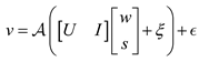
We denote the fixed d-dimensional subspace of ℝⁿ as . In application of interest we always suppose d ≪ n, say is a fixed low-rank subspace. Let the columns of an n × d matrix U be orthonormal and span . {𝒜|ℝⁿ → ℝ^m, m < n} is a linear compressive measurement operator which should satisfy the restricted isometry property (RIP) [2] with constant δ_K

(2)

We want to recover the K-sparse signal s ϵ ℝ ⁿ buried in the low-rank background signal l = Uw and small Gaussian noise corruption ξ from the compressive measurement v with small Gaussian measurement noise ϵ as Equation (1), here, K-sparse means ‖s‖₀ ≤ K.

2.2. Variant of CoSaMP for Fixed Subspace

To tackle this special sparse recovery problem, we adopt the basic idea of CoSaMP [11]. Ordinary CoSaMP could efficiently solve the following underdetermined linear equation system if x is a K-sparse signal and the measurement operator satisfies RIP with constant δ_K.

y = 𝒜(x) + ϵ

(3)

Comparing the problems between Equations (1) and (3), for a fixed low-rank subspace, if we can remove the dense signal generated by the subspace, then problem Equation (1) will be converted to the classic sparse recovery problem Equation (3). We consider the greedy approach to iteratively remove the effect of the dense signal then estimate the sparse signal in the framework of CoSaMP. The main idea is as follows: we iteratively estimate the weights w^k which constructs the low-rank background signal l = Uw^k; then form the signal proxy from the current residue u^k = v − 𝒜(Uw^k + s^k); then identify the support of the sparse signal just as ordinary CoSaMP; finally estimate the signal by least squares over the identified support.

We summarize the proposed CoSaMP_subspace as Algorithm 1. Here 𝒜^* denotes the adjoint of the operator 𝒜. The notation supp(y;K) denotes the largest K-term support of the vector y. Let 𝒜_|T denote the restriction of the operator to the support T.

Algorithm 1. Given a fixed subspace spanned by the column space of an n × d orthonormal matrix U, the variant of CoSaMP solver for the sparse recovery problem Equation (1). (s*, w*) = CoSaMP_subspace(v, U, 𝒜, 𝒜*, K, ε, maxIter).
1:	Initialize s,w,u: s0 =0, w0 =0, u0 =0.
2:	while and k < maxIter do
3:	Estimate weights w: wk+1 = $\mathrm{(𝒜}$(U))−1(v − 𝒜(sk))
4:	Form signal proxy: y = 𝒜*(uk)
5:	Support identification: Ω = supp(y; 2K)
6:	Merge support:
7:	Signal estimation by least squares:
8:	Update residue:
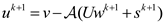
9:	k = k + 1
10:	end while
11:	(s*, w*) = (sk, wk)

It can be easily seen from Algorithm 1 that, compared with CoSaMP [11], the variant tries to estimate the weights of the dense signal in step 3 and remove its effects from the CS measurement in Step 8. The main framework follows CoSaMP. Thus, the proposed algorithm inherits the merits of CoSaMP, for example the total cost per iteration is O(nlogn) [11], and the total  storage is, at worst, O(nd) because of holding the fixed low-rank subspace.

2.3. Relation to Ordinary CS

For this special form of sparse recovery problem Equation (1), it could be also tackled via ordinary CS algorithms. We discuss its relation to our proposed algorithm in this subsection.

We rewrite problem Equation (1) as:

(4)

Here I is the n × n identity matrix. Let B = [U I] and x = [w s]^T, so x is a “K + d”-sparse signal. Then problem (1) converts to the classic CS model regardless of the effect of data noise ξ.

v = 𝒜 (Bx + ξ) + ϵ ≈ 𝒜(Bx) + ϵ

(5)

As 𝒜 is a CS operator satisfying RIP, for example, a random Gaussian matrix, and B =[U I] is a fixed basis, it is well-known in CS theory that 𝒜 is largely incoherent with B [2]. Then, x can be exactly recovered via CS techniques given enough linear measurements, for example CoSaMP, so does s.

However, we want to point out that though ordinary CS could also estimate the sparse signal s if we make the proper linear algebraic transform as above, the proposed algorithm works better when the sparse signal is also corrupted by small noise ξ and not only the measurement noise ϵ. It is because in step 3 of Algorithm 1 we explicitly make the least square estimation to cancel the noise effect. We put the comparisons in the experiments section.

3. Experiments Evaluation

In this section, we evaluate the performance of Algorithm 1 extensively on both simulated data and video CS application. For simulated data, we use Equation (1) to generate a series of CS vectors v. Like most CS literature, we use the noiselet operator [15,16] as the measurement operator 𝒜, which compresses an n × 1 vector to a p × 1 vector, and we denote as the CS measurement ratio. U is an n × d matrix whose d columns are realizations of i.i.d. $𝒩$(0,I_n) random variables that are then orthornomalized. The weight vector w is a d × 1 vector whose entries are realizations of i.i.d. $𝒩$(0,I_n) random variables, which are Gaussian distributed with mean zero and variance 1. The K-sparse signal s is an n × 1 vector whose supports are chosen uniformly at random without replacement and we denote as the sparsity of the signal. We use relative error to quantify the sparse recovery performance as follows:

(6)

Note that we manually add “1” to the denominator of RelErr because s may be 0-sparse in our following experiments.

In all the following experiments, we use Matlab R2010b on a Macbook Pro laptop with a 2.3 GHz Intel Core i5 CPU and 8 GB RAM. We always set the rank of the fixed subspace as d = 5, and the ambient dimension of signal is n = 512, unless otherwise noted.

3.1. Algorithm Behavior on Simulated Data

As a special CS algorithm, given a fixed subspace the performance of Algorithm 1 mainly relates to the sparsity of the signal ρ_s and the CS measurement ratio ρ_cs. We will also investigate how the rank of fixed subspace affects the performance of Algorithm 1.

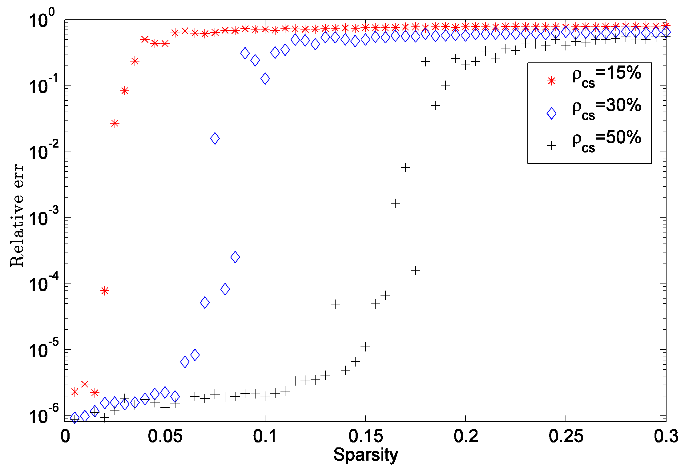
3.1.1. Recovery on Signal Sparsity

In the first experiment, we investigate how signal sparsity affects the success of recovery. Here we fix the CS measurement ratio ρ_cs as 15%, 30%, and 50%, respectively, and manually tune the signal sparsity from 0% to 30%. Figure 1 shows the fact that for truly sparse signal s, even a very small ratio of CS measurements could recover s from the low-rank background signal. For example, a 25-sparse signal can be successfully recovered from only 150 CS measurements.

Figure 1. Sparse recovery performance with respect to signal sparsity.

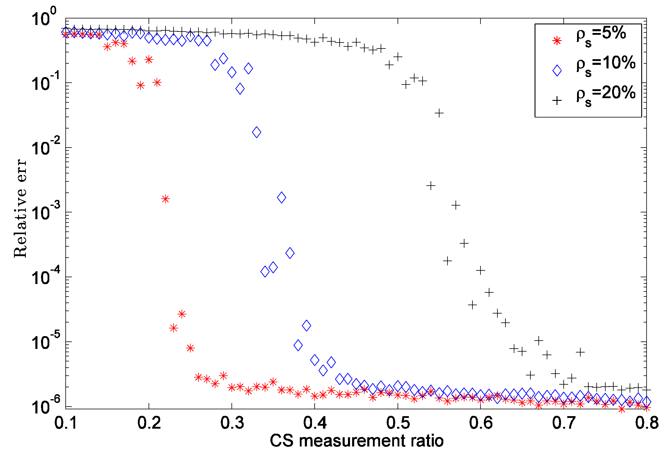
3.1.2. Recovery on CS Measurements

In the second experiment, we investigate how CS measurement ratio affects the success of recovery. Here we fix the signal sparsity ρ_s as 5%, 10%, and 20%, respectively, and manually tune the CS measurement ratio from 10% to 80%. Figure 2 shows the fact that, given enough CS measurements, even a near sparse signal can be precisely estimated, for example a 100-sparse signal can be recovered with high quality from 350 CS measurements

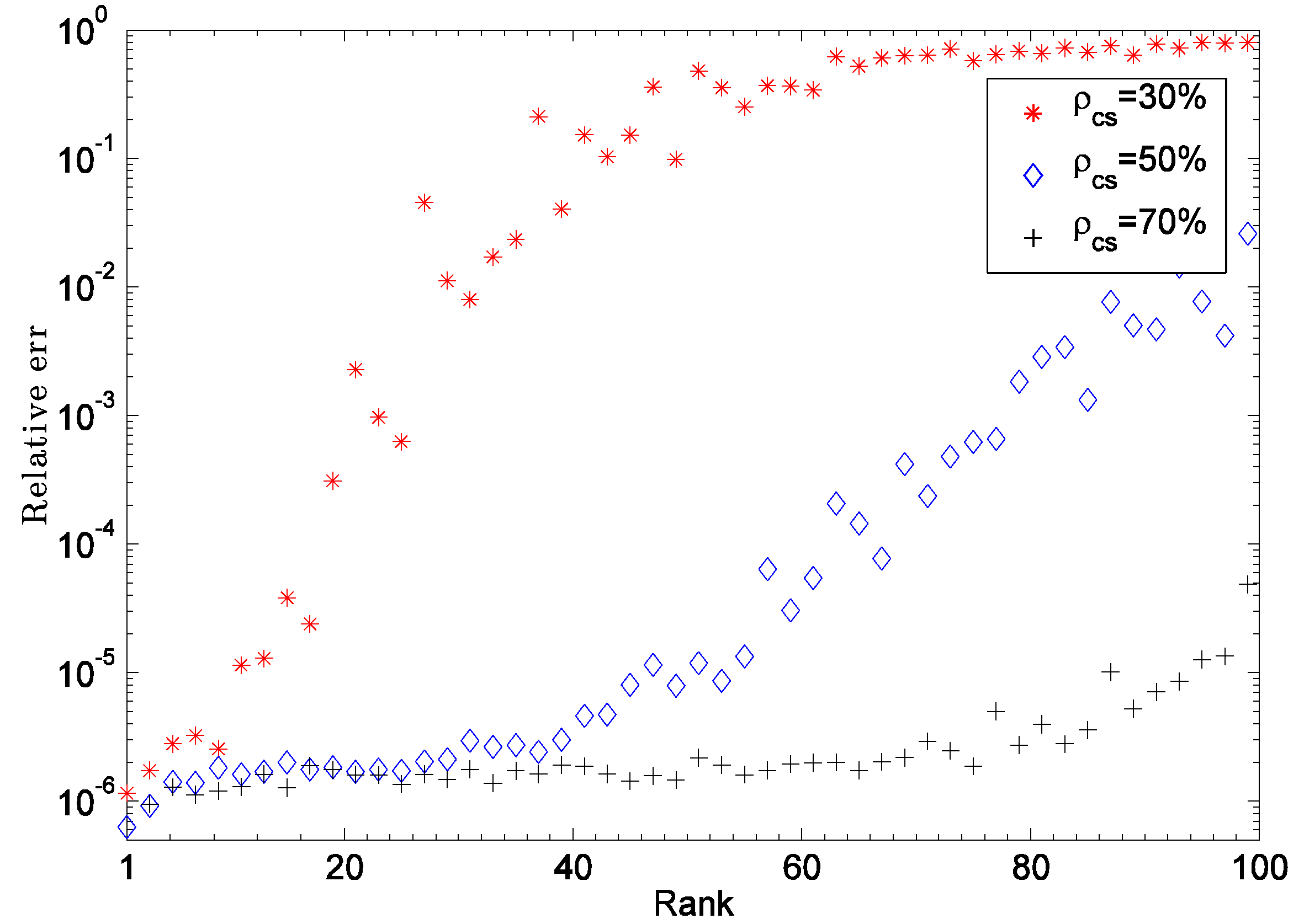
3.1.3. Recovery on the Rank of Fixed Subspace

As the special sparse recovery problem depends on the fixed subspace, in the third simulated experiment we demonstrate how the rank of the fixed subspace affects recovery. To observe the algorithm behavior, we fix the signal sparsity ρ_s as 5% and generate a series of simulated signals with different rank setting from rank = 1 to rank = 100. Figure 3 shows the recovery results with CS measurement ratio ρ_cs as 30%, 50%, and 70% respectively. It can be clearly seen that given moderate enough CS measurements the proposed algorithm can guarantee the recovery with up to a relative high rank of the fixed subspace. For example, with the CS measurement ρ_cs =50% the sparse signal can be stably separated from the fixed subspace with up to rank = 40.

Figure 2. Sparse recovery performance with respect to CS measurement ratio.

Figure 3. Sparse recovery performance with respect to the rank of fixed subspace.

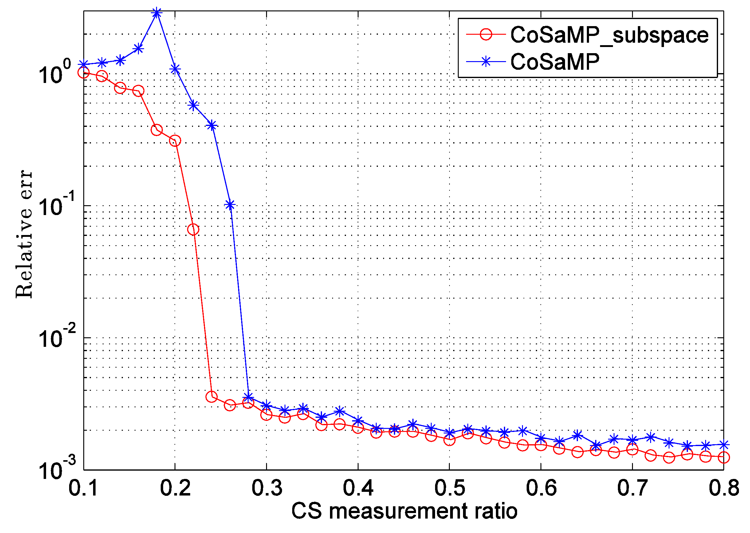
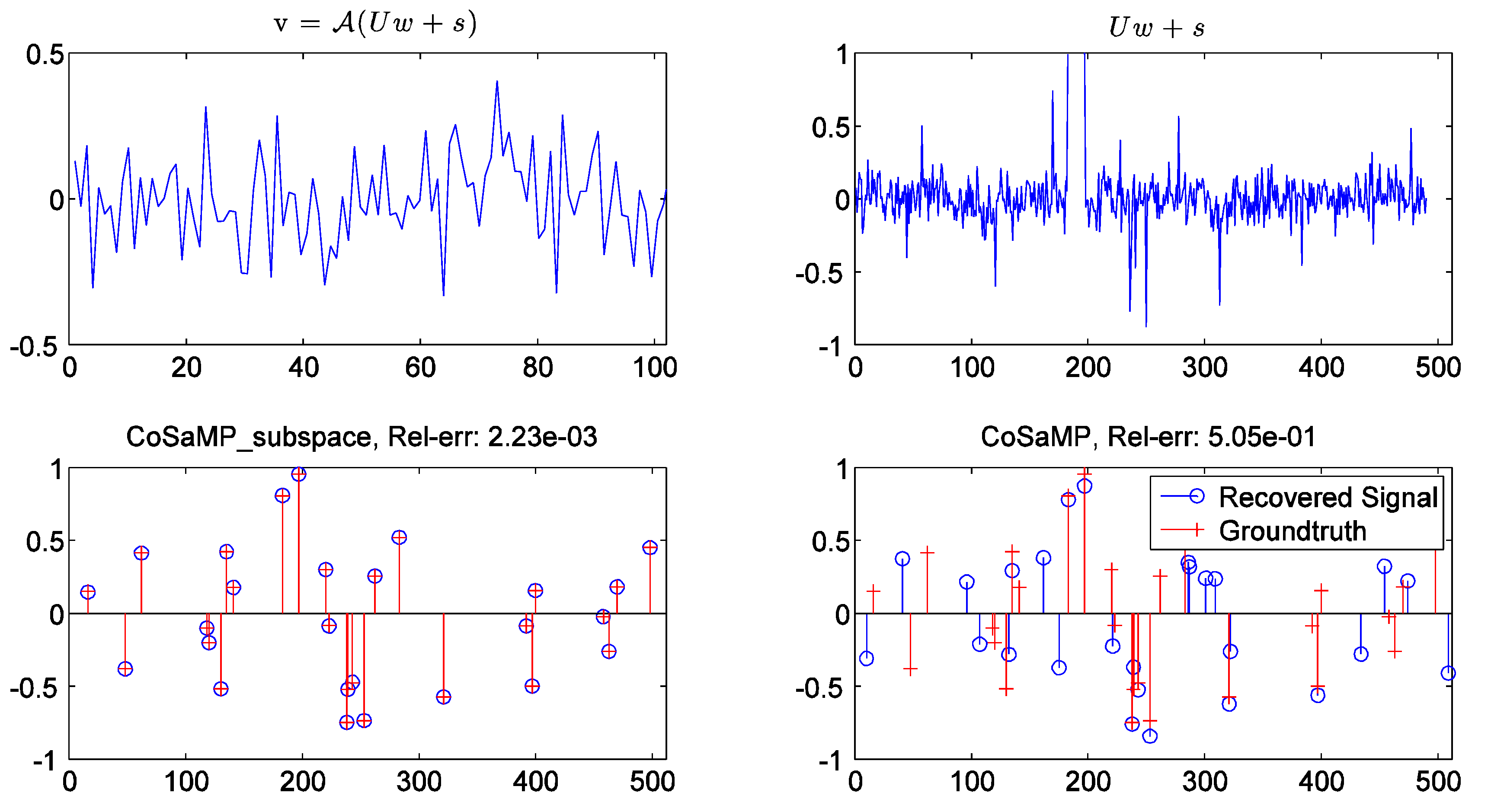
3.2. Comparisons with Ordinary CS

From the previous discussion we know that, if we transform the original problem Equation (1) to Equation (5), the sparse signal could also be recovered by ordinary CS. However, as we just pointed out above, if the noise not only occurs in measurement phase but also lies in data itself, Algorithm 1 can give a better estimation. Here, we address this comparison by adding relative strong noise corruption to the data in which the variance of ξ in Equation (1) is 10⁻³. In addition to this noise setting, we fix the sparsity ρ_s = 5% and vary the CS measurement ratio ρ_cs from 10% to 80% to observe the performance comparison between Algorithm 1 and ordinary CS. From Figure 4 it can be easily seen that Algorithm 1 outperforms ordinary CS (CoSaMP) when data itself is also corrupted by relative strong Gaussian noise, especially when the CS measurement ratio is small.

Figure 4. Performance comparison between CoSaMP_subspace and ordinary CS (CoSaMP) for noisy sparse recovery problem.

We make a more clear comparison in Figure 5. Here, we simulate a sparse signal s with sparsity ρ_s =5% and take CS measurements with measurement ratio ρ_cs = 20%. The variance of additional Gaussian noise ξ and measurement noise ϵ; are all set as 10⁻³. From this noisy CS measurement setting, Figure 5 shows that the estimated sparse signal by our algorithm can exactly match the original signal at RelErr = 2.23 × 10⁻³ which is approaching the data noise level 10⁻³. However, ordinary CoSaMP makes a worse estimation, say RelErr = 5.06 × 10⁻¹, as relative strong data noise ξ would introduce more uncertainty when the algorithm tries to identify the sparse support Ω.

Figure 5. Noisy sparse signal recovery comparison between CoSaMP_subspace and ordinary CS (CoSaMP). Top-left is the compressive measured signal v; top-right is the uncompressed signal—“dense structured signal + sparse signal”; bottom-left is the recovered sparse signal by our algorithm; bottom-right is the recovered sparse signal by ordinary CoSaMP.

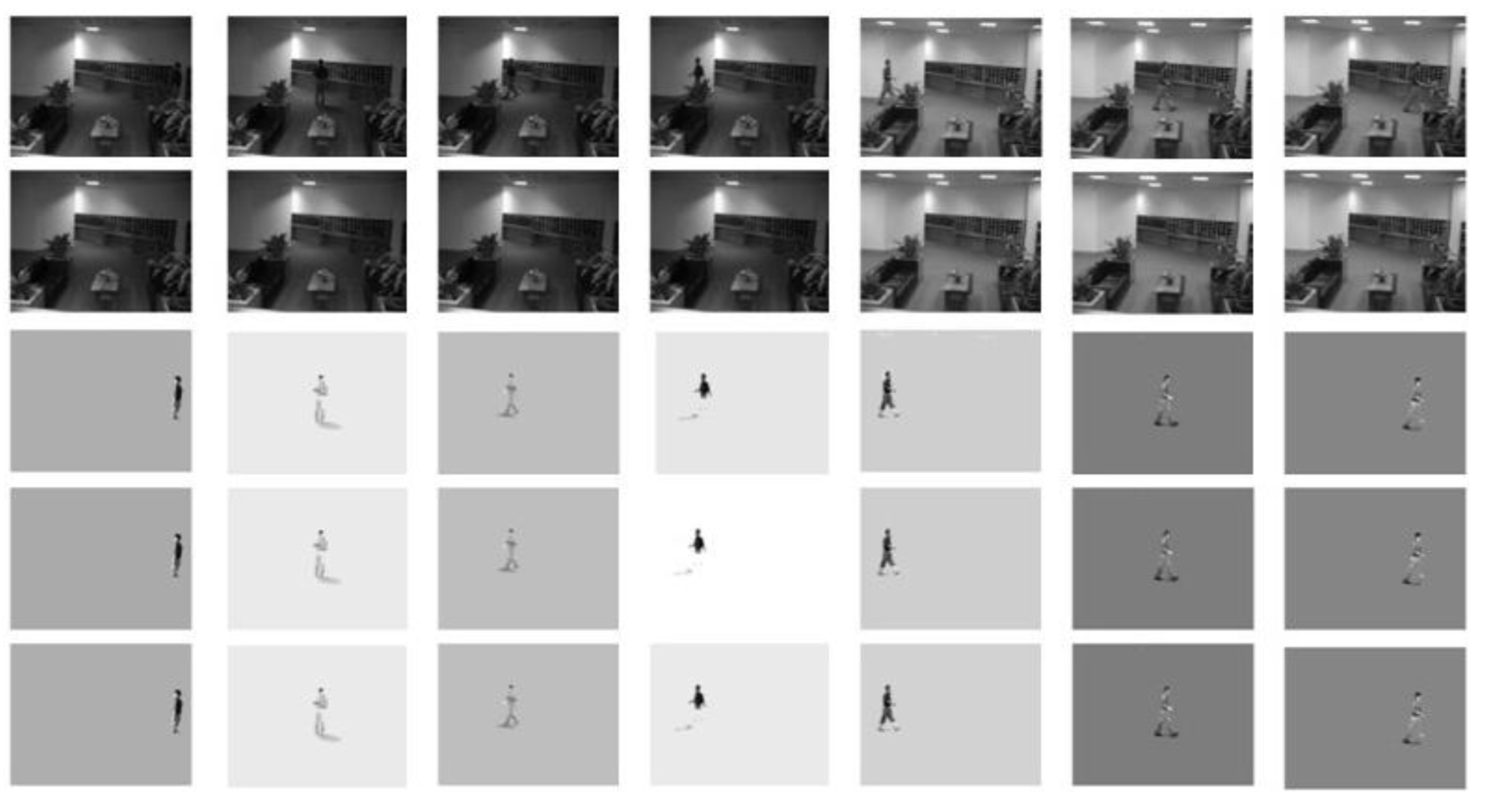
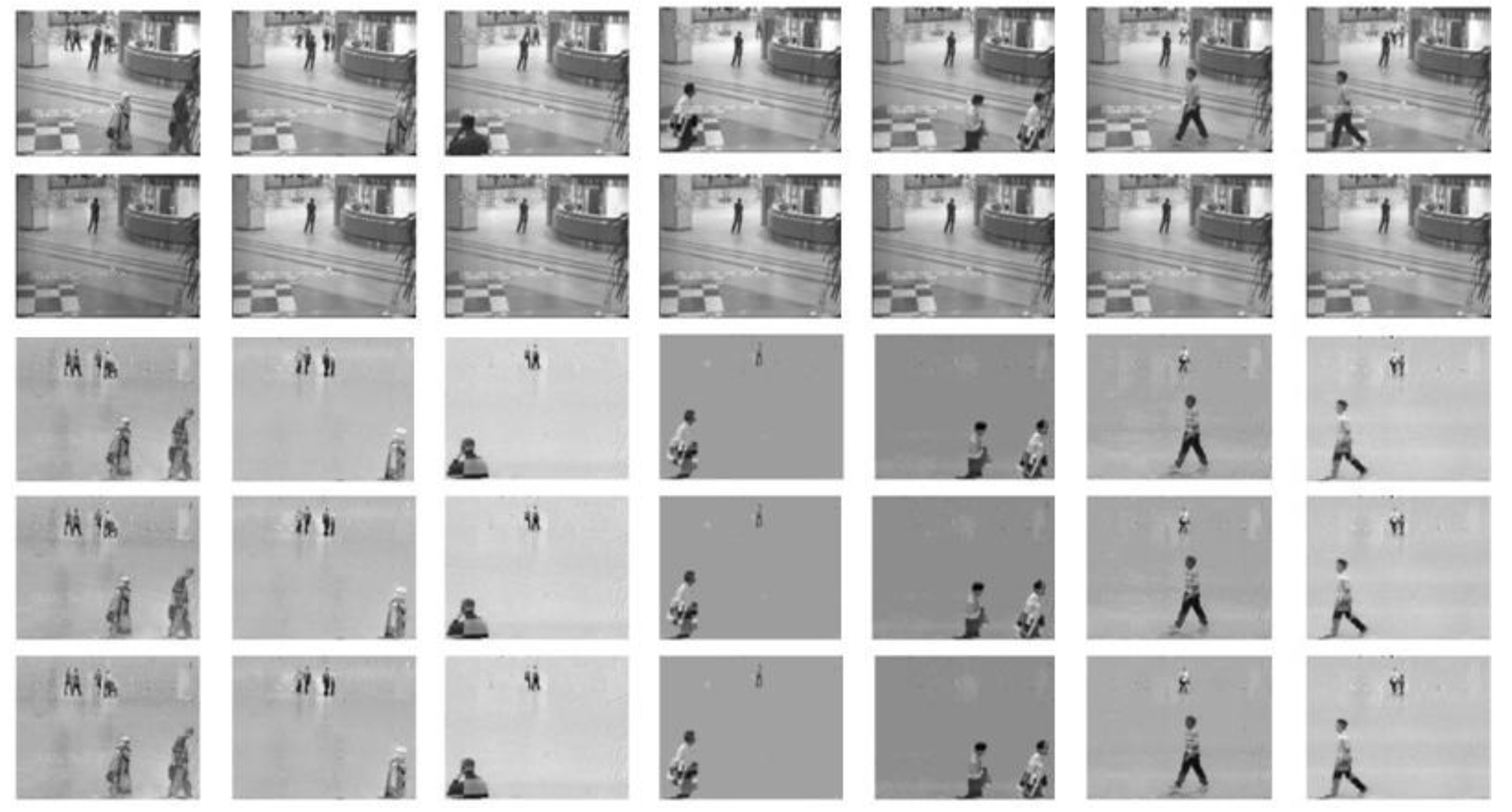
3.3. Video Compressive Sensing

In video surveillance, background images are always modeled as a low-rank subspace and foreground moving objects are regarded as sparse signals. Then, the following “Low-rank + Sparse” model [17,18] can well represent the video frame captured by stationary camera, which has been studied extensively in recent literature.

I = Uw + s

(6)

Here, we consider applying Algorithm 1 to video compressive sensing application [19], for example, the video frames are captured by single-pixel camera [20] in CS literature.

We simulate video CS by performing noiselet operator 𝒜 [15] on each normal surveillance video frame. Then recovering the foreground moving objects is just the problem Equation (1) in this paper. We test our simulation on the two well-known datasets (Dataset can be downloaded from http://perception.i2r.a-star.edu.sg/bk_model/bk_index.html.) “airport” and “lobby” in which the image dimension of the two datasets is 144 × 176. In order to perform CS measurement on each video frame, conforming to the noiselet convention, we first manually resize each frame as 128 × 128, which is the power of 2, thus, the ambient dimension of each video frame I_t in our experiment is 128 × 128. Then, for each video frame I_t, we take the CS measurement v_t= 𝒜 (I_t) with CS measurement ratio ρ_cs. As the two surveillance videos are static, our fixed low-rank subspace assumption holds. We obtain the fixed low-rank orthonormal matrix U as follows. For each dataset, we choose 200 video frames and perform the Robust PCA algorithm Inexact ALM (IALM) [21] on those frames to get the clean background images, which can be regarded as lying in a low-rank subspace. Then, the rank d orthonormal matrix U is obtained by performing SVD on those background images and keeping the columns corresponding to the largest d singular values. In our experiments we set d = 5.

In order to show how CS measurement ratio affects the recovery results, for the moderate sparse dataset “airport” we set the sparsity ρ_s = 20% and take CS measurement with ratios ρ_cs = 30%, ρ_cs = 20%, and ρ_cs =15%, respectively; and for the truly sparse dataset “lobby” we set the sparsity ρ_s = 5% and take CS measurement with ratios ρ_cs = 20%, ρ_cs = 5%, and ρ_cs = 1%, respectively. For “airport”, Figure 6 shows that the moving foreground objects can be well estimated though there are some ghost-effects in the recovery images, for example the first column. This effect is because IALM can not totally remove foreground from background due to the objects moving slowly in the scene which does not strictly follow the PCP recovery theorem [17]. The second row of Figure 6 shows the background estimated by IALM in which there does exist some slight shadows. The FPS (frame per second) regarding the first 200 frames of “airport” is 2.16 fps at ρ_cs = 15% in our Matlab implementation. For “lobby”, from Figure 7, we can see that even if we just take ρ_cs = 1% CS measurement (the bottom row), the recovered results are comparable to taking much more measurement ρ_cs = 20% (the third row). More promisingly, while separating the total 1546 frames the proposed algorithm only takes 72.16 s, say the FPS is 21.42 fps for “lobby” at the extremely low CS measurement ratio ρ_cs = 1%. Note that though there is large illumination variation in this dataset the recovery performance is still stable.

Figure 6. Foreground recovery from video compressive sensing on “airport” dataset. The 1^st row is the original video frames; the 2^nd row shows the estimated background images by IALM [21] that are used to train our fixed low-rank subspace; the 3^rd row shows the recovered foreground with CS measurement ratio ρ_cs = 30%; the 4^th row shows the recovered foreground with ρ_cs = 20%; and the last row shows the recovered foreground with ρ_cs = 15%. The sparsity is set as ρ_s = 20%.

Figure 7. Foreground recovery from video compressive sensing on “lobby” dataset. The 1^st row is original video frames; the 2^nd row shows the estimated background images by IALM [21] that are used to train our fixed low-rank subspace; the 3^rd row shows the recovered foreground with CS measurement ratio ρ_cs = 20%; the 4^th row shows the recovered foreground with ρ_cs = 5%; and the last row shows the recovered foreground with ρ_cs = 1%. The sparsity is set as ρ_s = 5%.

4. Conclusions and Future Works

This paper presents a variant of CoSaMP algorithm, which can tackle a special sparse signal recovery problem v = 𝒜(Uw+ s). The algorithm could separate the sparse signal and low-rank background signal from their sum given very few CS measurements. From experiments we show that the recovery performance is similar to ordinary CoSaMP and performs better if the sparse signal also corrupted by Gaussian noise not only the measurement noise.

This proposed algorithm assumes that the low-rank subspace is known as a prior. However, what if the subspace is not known or even the subspace is time-varying? It is a challenging problem, to simultaneously estimate the subspace and recover the sparse signal only from a few CS measurements, which is attracting the attention of CS community [22,23,24]. We are very interested in incorporating the recent online subspace learning technique [18,25] into this CS framework. We put this endeavor for future work.

References

- Donoho, D.L. Compressed sensing. IEEE Trans. Inf. Theory 2006, 52, 1289–1306. [Google Scholar] [CrossRef]
- Candès, E.J. The restricted isometry property and its implications for compressed sensing. Comptes Rendus Math. 2008, 346, 589–592. [Google Scholar] [CrossRef]
- Candès, E.J.; Wakin, M.B. An introduction to compressive sampling. IEEE Signal Process. Mag. 2008, 25, 21–30. [Google Scholar] [CrossRef]
- Candès, E.J.; Romberg, J.; Tao, T. Robust uncertainty principles: Exact signal reconstruction from highly incomplete frequency information. IEEE Trans. Inf. Theory 2006, 52, 489–509. [Google Scholar] [CrossRef]
- Baraniuk, R.G. Compressive sensing [lecture notes]. IEEE Signal Process. Mag. 2007, 24, 118–121. [Google Scholar] [CrossRef]
- Lustig, M.; Donoho, D.; Pauly, J.M. Sparse MRI: The application of compressed sensing for rapid MR imaging. Magn. Reson. Med. 2007, 58, 1182–1195. [Google Scholar] [CrossRef] [PubMed]
- Haupt, J.; Bajwa, W.U.; Rabbat, M.; Nowak, R. Compressed sensing for networked data. IEEE Signal Process. Mag. 2008, 25, 92–101. [Google Scholar] [CrossRef]
- Quer, G.; Masiero, R.; Munaretto, D.; Rossi, M.; Widmer, J.; Zorzi, M. On the Interplay between Routing and Signal Representation for Compressive Sensing in Wireless Sensor Networks. In Proceedings of the IEEE Information Theory and Applications Workshop, La Jolla, CA, USA, 8–13 February 2009; pp. 206–215.
- Ji, S.; Xue, Y.; Carin, L. Bayesian compressive sensing. IEEE Trans. Signal Process. 2008, 56, 2346–2356. [Google Scholar] [CrossRef]
- Ji, S.; Dunson, D.; Carin, L. Multitask compressive sensing. IEEE Trans. Signal Process. 2009, 57, 92–106. [Google Scholar] [CrossRef]
- Needell, D.; Tropp, J.A. CoSaMP: Iterative signal recovery from incomplete and inaccurate samples. Appl. Comput. Harmon. Anal. 2009, 26, 301–321. [Google Scholar] [CrossRef]
- Donoho, D.L.; Tsaig, Y. Fast Solution of l1-Norm Minimization Problems When the Solution May Be Sparse; Department of Statistics, Stanford University: Stanford, CA, USA, 2006. [Google Scholar]
- Qiu, C.; Vaswani, N. Recursive Sparse Recovery in Large but Correlated Noise. In Proceedings of the IEEE 2011 49th Annual Allerton Conference on Communication, Control, and Computing (Allerton), Monticello, IL, USA, 28–30 September 2011; pp. 752–759.
- Boyd, S.; Parikh, N.; Chu, E.; Peleato, B.; Eckstein, J. Distributed optimization and statistical learning via the alternating direction method of multipliers. Found. Trends Mach. Learn. 2011, 3, 1–122. [Google Scholar] [CrossRef]
- Coifman, R.; Geshwind, F.; Meyer, Y. Noiselets. Appl. Comput. Harmon. Anal. 2001, 10, 27–44. [Google Scholar] [CrossRef]
- Romberg, J. Imaging via compressive sampling. IEEE Signal Process. Mag. 2008, 25, 14–20. [Google Scholar] [CrossRef]
- Candès, E.J.; Li, X.; Ma, Y.; Wright, J. Robust principal component analysis? J. ACM 2011, 58, 11. [Google Scholar] [CrossRef]
- He, J.; Balzano, L.; Szlam, A. Incremental Gradient on the Grassmannian for Online Foreground and Background Separation in Subsampled Video. In Proceedings of the 2012 IEEE Conference on Computer Vision and Pattern Recognition (CVPR), Providence, RI, USA, 16–21 June 2012; pp. 1568–1575.
- Cevher, V.; Sankaranarayanan, A.; Duarte, M.F.; Reddy, D.; Baraniuk, R.G.; Chellappa, R. Compressive Sensing for Background Subtraction. In Computer Vision–ECCV 2008; Springer: Marseille, France, 2008; pp. 155–168. [Google Scholar]
- Duarte, M.F.; Davenport, M.A.; Takhar, D.; Laska, J.N.; Sun, T.; Kelly, K.F.; Baraniuk, R.G. Single-pixel imaging via compressive sampling. IEEE Signal Process. Mag. 2008, 25, 83–91. [Google Scholar] [CrossRef]
- Lin, Z.; Chen, M.; Ma, Y. The augmented lagrange multiplier method for exact recovery of corrupted low-rank matrices. 2010. arXiv preprint arXiv:1009.5055. arXiv.org e-Print archive. Available online: http://arxiv.org/abs/1009.5055 (accessed on 10 September 2013).
- Waters, A.E.; Sankaranarayanan, A.C.; Baraniuk, R. SpaRCS: Recovering Low-Rank and Sparse Matrices from Compressive Measurements. In Proceedings of the Advances in Neural Information Processing Systems, Granada, Spain, 12–14 December 2011; pp. 1089–1097.
- Zhan, J.; Vaswani, N.; Atkinson, I. Separating Sparse and Low-Dimensional Signal Sequences from Time-Varying Undersampled Projections of Their Sums. In Proceedings of the 2013 IEEE International Conference on Acoustics,Speech and Signal Processing (ICASSP), Vancouver, BC, Canada, 26–31 May 2013; pp. 5905–5909.
- Wright, J.; Ganesh, A.; Min, K.; Ma, Y. Compressive principal component pursuit. Inf. Inference 2013, 2, 32–68. [Google Scholar] [CrossRef]
- Balzano, L.; Nowak, R.; Recht, B. Online Identification and Tracking of Subspaces from Highly Incomplete Information. In Proceedings of the IEEE 2010 48th Annual Allerton Conference on Communication, Control, and Computing (Allerton), Monticello, IL, USA, 29 September–1 October 2010; pp. 704–711.
© 2013 by the authors; licensee MDPI, Basel, Switzerland. This article is an open access article distributed under the terms and conditions of the Creative Commons Attribution license (http://creativecommons.org/licenses/by/3.0/