1. Introduction
As a result of the sharply falling costs of sequencing, large sequence databases are rapidly emerging, and they will soon grow to thousands of genomes and more. Sequencing machines are already producing terabytes of data per day, at a few thousand dollars per genome, and will cost less very soon (see, e.g., [
1]). This raises a number of challenges in bioinformatics, particularly because those sequence databases are meant to be the subject of various analysis processes that require sophisticated data structures built on them.
The
suffix tree [
2,
3,
4] is probably the most important of those data structures. Many complex sequence analysis problems are solved through sophisticated traversals over the suffix tree [
5]. However, a serious problem of suffix trees, aggravated on large sequence collections, is that they take much space. A naive implementation can easily require 20 bytes per character, and a very optimized one reaches 10 bytes [
6]. A way to reduce this space to about 4 bytes per character is to use a simplified structure called a
suffix array [
7]. However, suffix arrays do not contain sufficient information to carry out all the complex tasks suffix trees are used for. Enhanced suffix arrays [
8] extend suffix arrays so as to recover the full suffix tree functionality, raising the space to about 6 bytes per character in practice. Other heuristic space-saving methods [
9] achieve about the same.
For example, on DNA sequences, each character could be encoded with just 2 bits, whereas the alternatives we have considered require 32 to 160 bits per character (bpc). This is an overhead of 1600% to 8000%! The situation is also a heresy in terms of Information Theory: Whereas the information contained in a sequence of n symbols over an alphabet of size σ is bits in the worst case, all the alternatives above require bits. (Our logarithms are in base 2)
A solution to the large space requirements is of course resorting to secondary memory. However, using suffix trees on secondary memory makes them orders of magnitude slower, as most of the required traversals are highly non-local. A more interesting research direction, which has made much progress in recent years, is to design compressed suffix trees (CSTs). Those compressed representations of suffix trees are able to approach not only the worst-case space of the sequence, but even its information content (i.e., they approach the space of the compressed sequence). CSTs are composed of a compressed suffix array (CSA) plus some extra information that encodes the suffix tree topology and longest common prefix (LCP) information (more details later). The existing solutions can be divided into three categories:
Explicit topology. The first CST proposal was by Sadakane [
10,
11]. It uses
bits to represent the suffix tree topology, plus
bits to represent the LCP values. In addition, it uses Sadakane’s CSA [
12], which requires
bits, where
is the zero-order entropy of the sequence. This structure supports most of the tree navigation operations in constant time (except, notably, going down to a child, which is an important operation), at the price of
bits of space on top of a CSA.
Sampling. A second proposal was by Russo
et al. [
13,
14]. It is based on sampling some suffix tree nodes and recovering the information on any other node by moving to the nearest sample using suffix links. It requires only
bits on top of a CSA. By using an FM-index [
15] as the CSA, one achieves
bits of space, where
is the
k-th order empirical entropy of the sequence (a measure of statistical compressibility [
16]), for sufficiently low
, for any constant
. The navigation operations are supported in polylogarithmic time (at best
in their paper).
Intervals. Yet a third proposal was by Fischer
et al. [
17,
18,
19]. It avoids the explicit representation of the tree topology by working all the time with the corresponding suffix array intervals. All the suffix tree navigation is reduced to three primitive operations on such intervals: Next/Previous smaller value and range minimum queries (more details later). The proposal achieves a space/time tradeoff that is between the two previous ones: It reduces the
extra bits of Sadakane to
, and the superlogarithmic operation times of Russo
et al. to
, for any constant
. More precisely, the space is
bits (for the same
k ranges as above).
We remark that the space figures include the storage of the sequence itself, as all modern CSAs are self-indexes, that is, they contain both the sequence and its suffix array.
For applications, the
practical performance of the above schemes is more relevant than the theoretical figures. The solution based on explicit topology was implemented by Välimäki
et al. [
20]. As expected from theory, the structure is very fast, achieving a few tens of microseconds per operation, but uses significant space (about 25–35 bpc, close to a suffix array). This undermines its applicability. Very recently, Gog [
21] showed that this implementation can be made much more space-efficient, using about 13–17 bpc. This still puts this solution in the range of the “large” CSTs in the context of this paper.
The structure based on sampling was implemented by Russo. As expected from theory again, it was shown to achieve very little space, around 4–6 bpc, which makes it extremely attractive when the sequence is large compared with the available main memory. On the other hand, the structure is much slower than the previous one: Each navigation operation takes the order of milliseconds.
In this paper we present the
first implementations of the third approach, based on intervals. As predicted by theory once again, we achieve practical implementations that lie between the two previous extremes (too large or too slow) and offer attractive space/time tradeoffs. One variant shows to be superior to the original implementation of Sadakane’s CST [
20] in both space and time: It uses 13–16 bpc (
i.e., half the space) and requires a few microseconds per operation (
i.e., several times faster). A second variant works within 8–12 bpc and requires a few hundreds of microseconds per operation, that is, smaller than our first variant and still several times faster than Russo’s implementation. We remark again that those space figures include the storage of the sequence, and that 8 bpc is the storage space of a byte-based representation of the plain sequence (although 2 bpc is easily achieved on DNA).
Achieving those good practical results is not immediate, however. We show that a direct implementation of the techniques as described in the theoretical proposal [
18] does not lead to the best performance. Instead, we propose a novel solution to the previous/next smaller value and range minimum queries, based on the
range min-max tree (
RMM tree), a recent data structure developed for succinct tree representations [
22,
23]. We adapt RMM trees to speed up the desired queries on sequences of LCP values.
The resulting representation not only performs better than a verbatim implementation of the theoretical proposal, but also has a great potential to handle highly repetitive sequence collections. Those collections, formed by many similar strings, arise in version control systems, periodic publications, and software repositories. They also arise naturally in bioinformatics, for example when sequencing the genomes of many individuals of the same or related species (two human genomes share 99.9% of their sequences, for example). It is likely that the largest genome collections that will emerge in the next years will be highly repetitive, and taking advantage of that repetitiveness will be the key to handle them.
Repetitiveness is not captured by statistical compression methods nor frequency-based entropy definitions [
16,
24] (
i.e., the frequencies of symbols do not change much if we add near-copies of an initial sequence). Rather, we need
repetition aware compression methods. Although this kind of compression is well-known (e.g., grammar-based and Ziv-Lempel-based compression), only recently there have appeared CSAs and other indexes that take advantage of repetitiveness [
24,
25,
26,
27]. Yet, those indexes do not support the full suffix tree functionality. On the other hand, none of the existing CSTs is tailored to repetitive text collections.
Our second contribution is to present the first, and the only to date, fully-functional compressed suffix tree whose compression effectiveness is related to the repetitiveness of the text collection. While its operations are much slower than most existing CSTs (requiring the order of milliseconds), the space required is also much lower on repetitive collections (1.4–1.9 bpc in our mildly repetitive test collections, and 0.6 bpc on a highly repetitive one). This can make the difference between fitting the collection in main memory or having to resort to disk.
The paper is organized as follows.
Section 2 gives the basis of suffix array and tree compression in general and repetitive text collections, and puts our contribution in context.
Section 3 compares various LCP representations and chooses suitable ones for our CST.
Section 4 proposes the novel RMM-tree based solution for
operations and shows it is superior to a verbatim implementation of the theoretical proposal.
Section 5 assembles our CST using the previous pieces, and
Section 6 evaluates and compares it with alternative implementations.
Section 7 extends the RMM concept to design a CST that adapts to repetitive collections, and
Section 8 evaluates it. Finally,
Section 9 concludes and discusses various new advances [
21,
28] that have been made on efficiently implementing the interval-based approach since the conference publication of our results [
29,
30].
2. Related Work and Our Contribution in Context
Our aim is to handle a collection of texts over an alphabet Σ of size σ. This is customarily represented as a single text concatenating all the texts in the collection. The symbol “$” is an endmarker that does not appear elsewhere. Such a representation simplifies the discussion on data structures, which can consider that a single text is handled.
2.1. Suffix Arrays and CSAs
A suffix array over a text is an array of the positions in T, lexicographically sorted by the suffix starting at the corresponding position of T. That is, for all . Note that every substring of T is the prefix of a suffix, and that all the suffixes starting with a given pattern P appear consecutively in A, hence a pair of binary searches find the area containing all the positions where P occurs in T.
There are several
compressed suffix arrays (
CSAs) [
31,
32], which offer essentially the following functionality: (1) Given a pattern
, find the interval
of the suffixes starting with
P; (2) Obtain
given
i; (3) Obtain
given
j. An important function the CSAs implement is
and its inverse, usually much faster than computing
A and
. This function lets us move virtually in the text, from the suffix
i that points to text position
, to the one pointing to
. Function Ψ is essential to support suffix tree functionality.
Most CSAs are self-indexes, meaning that they can also extract any substring of T and thus T does not need to be stored separately. Generally, one can extract any using applications of Ψ, where s is a sampling parameter that involves spending extra bits of space.
2.2. Suffix Trees and CSTs
A
suffix trie is a trie (or digital tree) storing all the suffixes of
T. This is a labeled tree where each text suffix is read in a root-to-leaf path, and the edges toward the children of a node are labeled by different characters. The concatenation of the string labels from the root up to a node
v is called the
path-label of
v,
. A
suffix tree is obtained by “compacting” unary paths in a suffix trie, which means they are converted into a single edge labeled by the string that concatenates the involved character labels. Furthermore, a node
v is converted into a leaf (and the rest of its descending unary path is eliminated) as soon as
becomes unique. Such leaf is annotated with the starting position
i of the only occurrence of
in
T, that is, suffix
starts with
. If the children of each suffix tree node are ordered lexicographically by their string label, then the sequence of leaf annotations of the suffix tree is precisely the suffix array of
T.
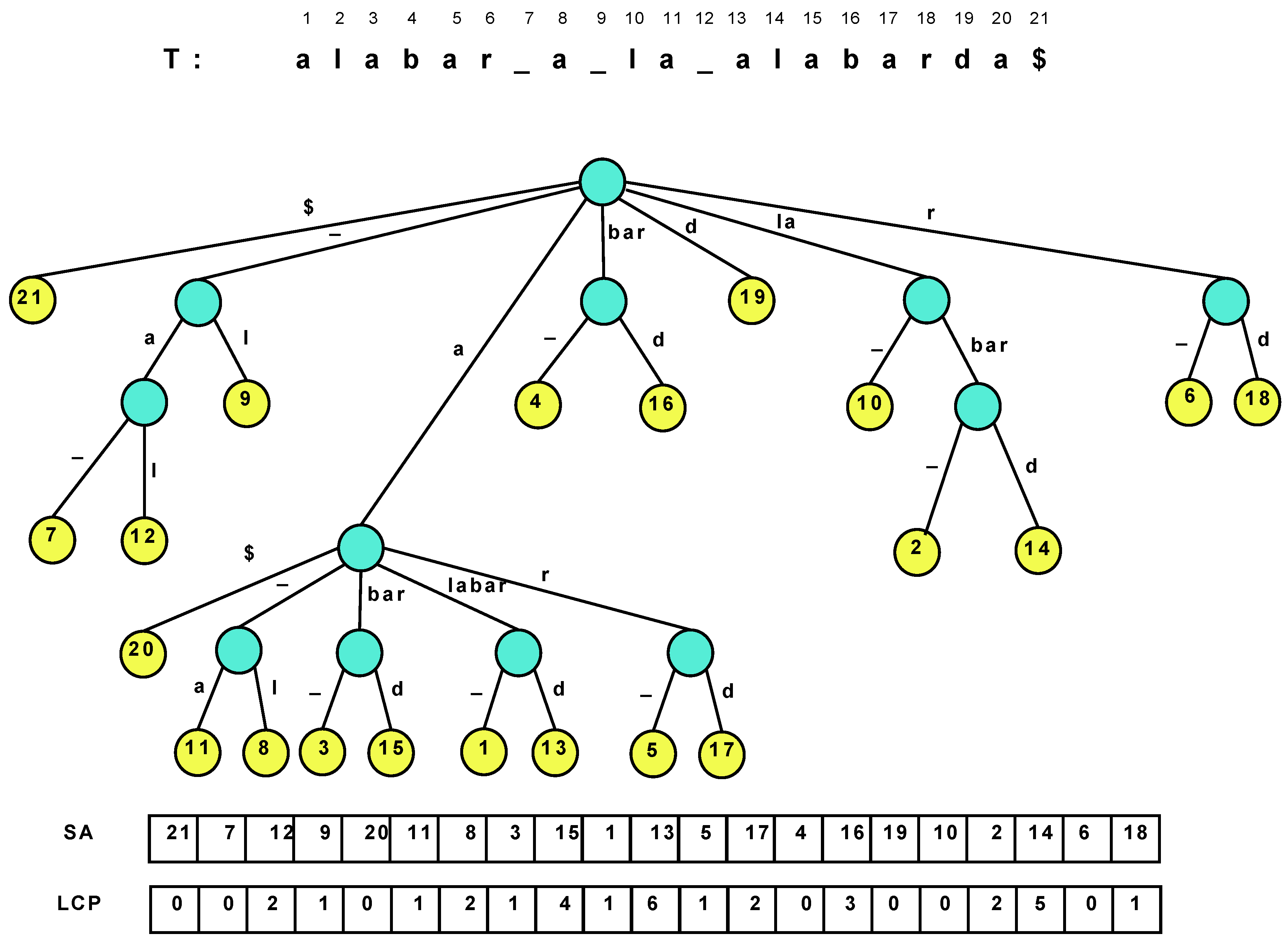
Figure 1 illustrates a suffix tree and suffix array. Several navigation operations over the nodes and leaves of the suffix tree are of interest.
Table 1 lists the most common ones.
Figure 1.
The suffix tree of the text “alabar a la alabarda$”, where the “$” is a terminator symbol. The white space is written as an underscore for clarity, and it is lexicographically smaller than the characters “a”–“z”.
Figure 1.
The suffix tree of the text “alabar a la alabarda$”, where the “$” is a terminator symbol. The white space is written as an underscore for clarity, and it is lexicographically smaller than the characters “a”–“z”.
Table 1.
Main operations over the nodes and leaves of the suffix tree.
Table 1.
Main operations over the nodes and leaves of the suffix tree.
| Operation | Description |
|---|
| Root() | the root of the suffix tree |
| Locate(v) | position i such that starts at , for a leaf v |
| Ancestor() | true if v is an ancestor of w |
| SDepth(v) | string-depth of v, i.e., |
| TDepth(v) | tree-depth of v, i.e., depth of node v in the suffix tree |
| Count(v) | number of leaves in the subtree rooted at v |
| Parent(v) | parent node of v |
| FChild(v) | alphabetically first child of v |
| NSibling(v) | alphabetically next sibling of v |
| SLink(v) | suffix-link of v, i.e., the node w s.th. if for |
| SLink(v) | iterated suffix-link, i.e., the node w s.th. if for |
| LCA() | lowest common ancestor of v and w |
| Child() | node w s.th. the first letter on edge is |
| Letter() | letter of v’s path-label, |
| LAQ() | the highest ancestor of v with string-depth |
| LAQ() | the ancestor of v with tree-depth d |
The suffix array alone is insufficient to efficiently emulate all the relevant suffix tree operations. To recover the full suffix tree functionality, we need two extra pieces of information: (1) The tree topology; (2) The longest common prefix (LCP) information, that is, is the length of the longest common prefix between and for and (or, seen another way, is the length of the string labeling the path from the root to the lowest common ancestor node of the ith and th suffix tree leaves). Indeed, the suffix tree topology can be implicit if we identify each suffix tree node with the suffix array interval containing the leaves that descend from it. This range uniquely identifies the node because there are no unary nodes in a suffix tree.
Consequently, a
compressed suffix tree (
CST) is obtained by enriching the CSA with some extra data. Sadakane [
11] added the topology of the tree (using
extra bits) and the LCP data. The LCP data was compressed to
bits by noticing that, if sorted by text order rather than suffix array order, the LCP numbers decrease by at most 1: Let
be the permuted
array, then
. Thus the numbers can be differentially encoded,
, and then represented in unary over a bitmap
. Then, to obtain
, we look for
, and this is extracted from
H via
rank/
select operations. Here
counts the number of bits
b in
and
is the position of the
i-th
b in
H. Both can be answered in constant time using
extra bits of space [
33]. Then
, assuming
.
Russo
et al. [
14] get rid of the parentheses, by instead identifying suffix tree nodes with their corresponding suffix array interval. By sampling some suffix tree nodes, most operations can be carried out by moving, using suffix links, towards a sampled node, finding the information stored in there, and transforming it as we move back to the original node. The suffix link operation, defined in
Table 1, can be computed using Ψ and the lowest common ancestor operation [
11].
2.3. Re-Pair and Repetition-Aware CSAs
Re-Pair [
34] is a grammar-based compression method that factors out repetitions in a sequence. It is based on the following heuristic: (1) Find the most repeated pair
in the sequence; (2) Replace all its occurrences by a new symbol
s; (3) Add a rule
to a dictionary
R; (4) Iterate until every pair is unique.
The result of the compression of a text T, over an alphabet Σ of size σ, is the dictionary R and the remaining sequence C, containing new symbols (s) and symbols in Σ. Every sub-sequence of C can be decompressed locally by the following procedure: Check if ; if so the symbol is original, else look in R for rule , and recursively continue expanding with the same steps.
The dictionary R corresponds to a context-free grammar, and the sequence C to the initial symbols of the derivation tree that represents T. The final structure can be regarded as a sequence of binary trees with roots .
González and Navarro [
35] used Re-Pair to compress the differentially encoded suffix array,
. They showed that Re-Pair achieves
on
,
r being the number of runs in Ψ. A run in Ψ is a maximal contiguous area where
. It was shown that the number of runs in Ψ is
for any
k [
36]. More importantly, repetitions in
T induce long runs in Ψ, and hence a smaller
r [
25]. An exact bound has been elusive, but Mäkinen
et al. [
25] gave an average-case upper bound for
r: If
T is formed by a random base sequence of length
and then other sequences that have
m random
mutations (which include indels, replacements, block moves,
etc.) with respect to the base sequence, then
r is at most
+
on average.
The RLCSA [
25] is a CSA where those runs in Ψ are factored out, to achieve
cells of space. More precisely, the size of the RLCSA is
bits. It supports accesses to
A in time
, with
extra bits for a sampling of
A.
2.4. An Interval-Based CST
Fischer
et al. [
18] prove that bitmap
H in Sadakane’s CST is compressible as it has at most
runs of 0’s or 1’s, where
r is the number of runs in Ψ as before.
Let
be the lengths of the runs of 0’s and
be the lengths of the runs of 1’s. Fischer
et al. [
18] create arrays
and
, with overall
1’s out of
, and thus can be compressed to
bits while supporting constant-time
rank and
select [
37]. When
r is very small it is better to use other bitmap representations (e.g., [
38]) requiring
bits, even if they do not offer constant times for
rank.
Their other improvement over Sadakane’s CST is to get rid of the tree topology and replace it with suffix array ranges. Fischer et al. show that all the navigation can be simulated by means of three operations: (1) The range minimum query gives the position of the minimum in ; (2) The previous smaller value finds the last value smaller than in ; and (3) The next smaller value finds the first value smaller than in . As examples, the parent of node can be computed as ; the LCA between nodes and is , where ; and the suffix link of is .
The three primitives could easily be solved in constant time using
extra bits of space on top of the
representation [
18] (more recently Ohlebusch
et al. [
28] showed how to solve them in constant time using
bits), but Fischer
et al. give sublogarithmic-time algorithms to solve them with only
extra bits.
A final observation of interest in that article [
18] is that the repetitions found in a differential encoding of the suffix array (
i.e., the runs in Ψ) also show up in the differential
, since if
A values differ by 1 in a range, the
areas must also differ by 1. Therefore, Re-Pair compression of the differential
should perform similarly as González and Navarro’s suffix array compression [
35].
2.5. Our Contribution
In this paper we design a practical and efficient CST building on the ideas of Fischer
et al. [
18], and show that its space/time performance is attractive. This challenge can be divided into (1) How to represent the LCP array efficiently in practice; and (2) How to compute efficiently
,
, and
over this LCP representation. For the first sub-problem we compare various implementations, whereas for the second we adapt a data structure called range min-max tree [
22], which was designed for another problem. We compare the resulting CST with previous ones and show that it offers relevant space/time tradeoffs. Finally, we design a variant of the range min-max tree that is suitable for highly repetitive collections (
i.e., with low
r value). This is obtained by replacing this regular tree by the (truncated) grammar tree of the Re-Pair compression of the differential LCP array. The resulting CST is the only one handling repetitive collections within space below 2 bpc.
3. Representing Array
The following alternatives were considered to represent :
Sad-Gon Encodes Sadakane’s [
11]
H bitmap in plain form, using the
rank/
select implementation of González [
39], which takes
bits on top of the
used by
H itself. This implementation answers
rank in constant time and
select in
time via binary search.
Sad-OS Like the previous one, but using the
dense array implementation of Okanohara and Sadakane [
38] for
H. This requires about the same space as the previous one and answers
select in time
.
FMN-RRR Encodes
H in compressed form as in Fischer
et al. [
18], that is, by encoding sparse bitmaps
Z and
O. We use the compressed representation by Raman
et al. [
37] as implemented by Claude [
40]. This costs
extra bits on top of the entropy of the two bitmaps,
. Operation
rank takes constant time and
select takes
time.
FMN-OS Like the previous one, but instead of Raman
et al.’s technique, we use the
sparse array implementation by Okanohara and Sadakane [
38]. This requires
bits and solves
select in time
.
PT Inspired in an LCP construction algorithm [
41], we store a particular sampling of
values, and compute the others using the sampled ones. Given a parameter
v, the sampling requires
bytes of space and computes any
by comparing at most some
and
. As we must obtain these symbols using Ψ up to
times, the idea is slow.
PhiSpare This is inspired in another construction [
42]. For a parameter
q, we store in text order an array
with the
values for all text positions
. Now assume
, with
. If
, then
. Otherwise,
is computed by comparing at most
symbols of the suffixes
and
. The space is
integers and the computation requires
applications of Ψ on average.
DAC The
directly addressable codes of Ladra
et al. [
43]. Most
values are small (
on average), and thus require few bits. Yet, some can be much larger. Thus we can fix a block length
b and divide each number of
ℓ bits into
blocks of
b bits. Each block is stored using
bits, the last one telling whether the number continues in the next block or finishes in the current one. Those blocks are then rearranged to allow for fast random access. There are two variants of this structure, both implemented by Ladra: One with fixed
b (
), and another using different
b values for the first, second,
etc. blocks, so as to minimize the total space (
). Note we represent
and not
, thus we do not need to compute
.
RPRe-Pair As mentioned, Re-Pair can be used to compress the differential
array,
[
18]. To obtain
we store sampled absolute
values and decompress the nonterminals since the last sample.
3.1. Experimental Comparison
Our computer is an Intel Core2 Duo at
GHz, with 8 GB of RAM and 6 MB cache, running Linux version
-24.
Table 2 lists the collections used for this experiment. They were obtained from the
Pizza & Chili site [
44]. We also give some information on their LCP values and number of runs in Ψ, which affects their compressibility. We tested the different LCP representations by accessing 100,000 random positions of the
array.
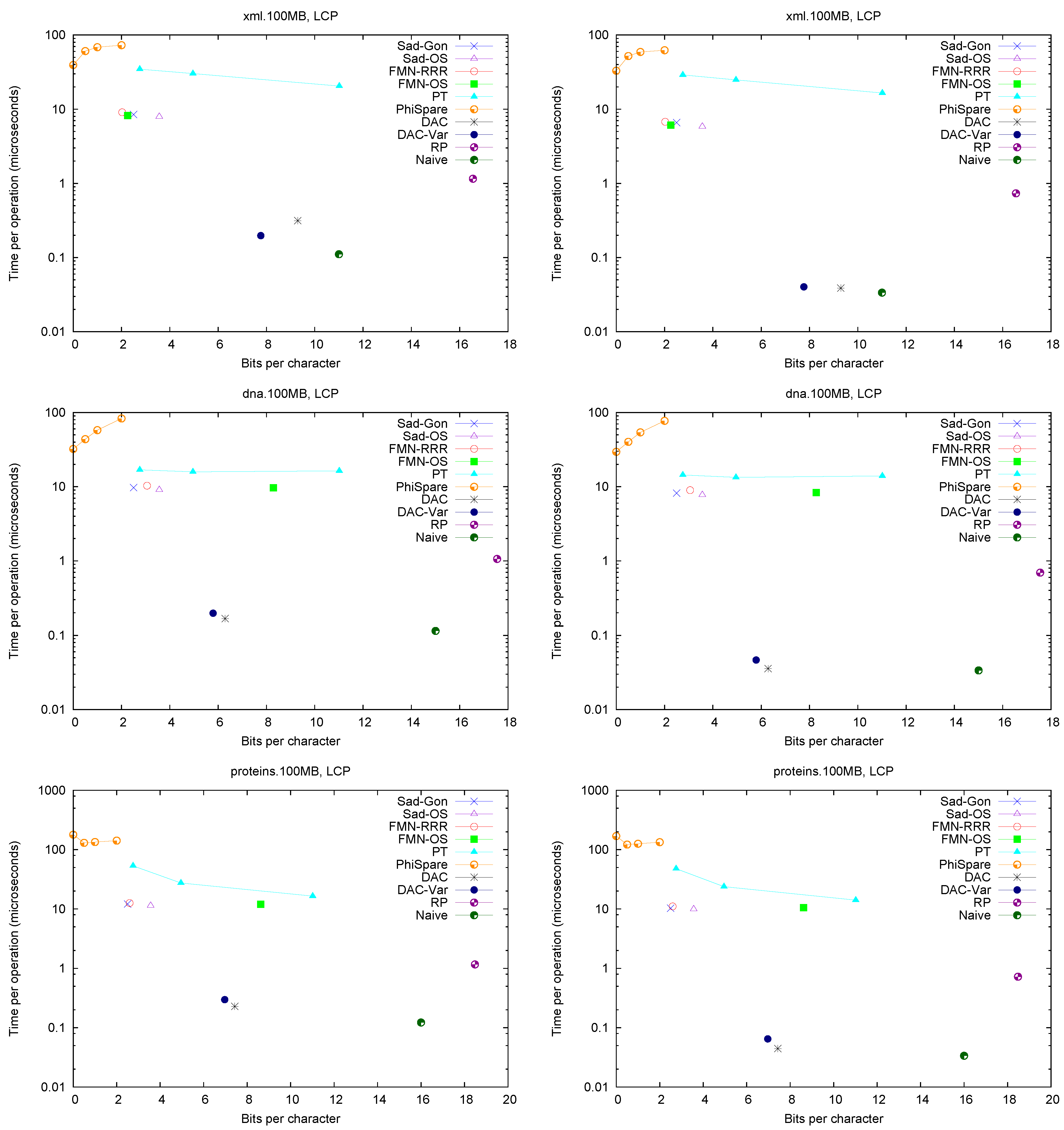
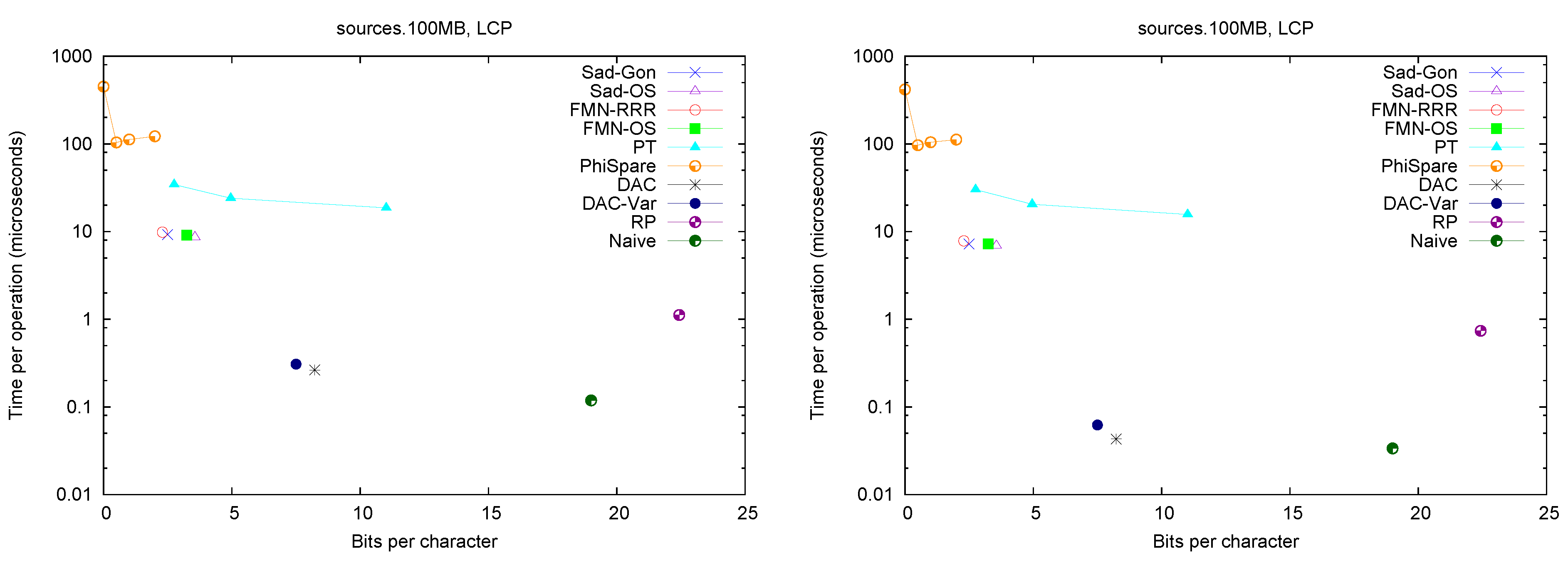
Figure 2 (left) shows the space/times achieved on the four texts. Only
and
PhiSpare display a space/time tradeoff; in the first we use
and for the second
. Because in various cases we need to access a sequence of consecutive LCP values, we show in
Figure 2 (right) the time per cell when accessing 32 consecutive cells. The plots also show solution
Naive, which stores LCP values using the number of bits required by the maximum value in the array.
Table 2.
Data files used for tests with their size in MB, plus some information on their compressibility.
Table 2.
Data files used for tests with their size in MB, plus some information on their compressibility.
| Collection | Size | Description | Avg LCP | Max LCP | Runs () |
|---|
| dna | 100 | DNA sequences from Gutenberg Project | | | 0.63 |
| xml | 100 | XML from dblp.uni-trier.de | | 1084 | 0.14 |
| proteins | 100 | Protein sequences from the Swissprot database | | | 0.59 |
| sources | 100 | Source code obtained by concatenating files of the Linux-2.6.11.6 and gcc-4.0.0 distributions | | | 0.23 |
Figure 2.
Space/Time for accessing array . On the left for random accesses and on the right for sequential accesses.
Figure 2.
Space/Time for accessing array . On the left for random accesses and on the right for sequential accesses.
We use Sadakane’s CSA implementation [
12], available at
Pizza & Chili, as our CSA, with sampling
. This is relevant because various LCP implementations need to compute
from the CSA.
A first observation is that Fischer et al.’s compression techniques for bitmap H do not compress significantly in practice (on non-repetitive collections). The value of r is not small enough to make the compressed representations noticeably smaller (and at times their space overhead over the entropy makes them larger, especially variant ).
These explicit representations of H require only bits of space and access in about 10 microseconds. Technique PT is always dominated by them and PhiSpare can achieve less space, but at the price of an unacceptable 10-fold increase in time.
The other dominant technique is /, which requires significantly more space ( bits) but can access within 0.1–0.2 microseconds. This is because it does not need to compute to find . Its time is even competitive with Naive, while using much less space. Technique , instead, does not perform well, doing even worse than Naive in time and space. This shows, again, that (in non-repetitive) collections the value r is not small enough: While the length of the Re-Pair compressed sequence is 30%–60% of the original one, the values require more bits than in Naive because Re-Pair creates many new symbols.
, and Naive are the only techniques that benefit from extracting consecutive values, so the former stay comparable with Naive in time even in this case. This owes to the better cache usage compared with the other representations, which must access spread text positions to decode a contiguous area.
For the sequel we will keep only and , which give the best time performance, and and , which have the most robust performance at representing H.
4. Computing , , and
Once a representation for
is chosen, one must carry out operations
,
, and
on top of it (as they require to access
). We first implemented verbatim the theoretical proposals of Fischer
et al. [
18]. For
, the idea is akin to the recursive
findclose solution for compressed trees [
45]: The array is divided into blocks and some values are chosen as
pioneers so that, if a position is not a pioneer, then its
answer is in the same block of that of its preceding pioneer (and thus it can be found by scanning that block). Pioneers are marked in a bitmap so as to map them to a reduced array of pioneers, where the problem is recursively solved. We experimentally verified that it is convenient to continue the recursion until the end instead of storing the explicit answers at some point. The block length
L yields a space/time tradeoff since, at each level of the recursion, we must obtain
values from
.
is symmetric, needing another similar structure.
For
we apply a recent implementation [
46,
47] on the LCP array, which does not need to access
yet requires
bits. In the actual theoretical proposal [
18] this space is reduced to
bits, but many accesses to
are necessary; we did not implement that idea verbatim as it has little chances of being practical.
The final data structure, which we call , is composed of the structure to answer plus the one for plus the structure to calculate .
4.1. A Novel Practical Solution
We propose now a different solution, inspired in Sadakane and Navarro’s
range min-max (RMM) tree data structure [
22]. We divide
into blocks of length
L. Now we form a hierarchy of blocks, where we store the minimum
value of each block
i in an array
. The array uses
bits. On top of array
m, we construct a perfect
L-
tree
where the leaves are the elements of
m and each internal node stores the minimum of the values stored in its children. The total space for
is
bits, so if
, the space used is
bits.
To answer , we look for the first such that , using to find it in time . We first search sequentially for the answer in the same block of i. If it is not there, we go up to the leaf that represents the block and search the right siblings of this leaf. If some of these sibling leaves contain a minimum value smaller than p, then the answer to is within their block, so we go down to their block and find sequentially the leftmost position j where . If, however, no sibling of the leaf contains a minimum smaller than p, we continue going up the tree and consider the right siblings of the parent of the current node. At some node we find a minimum smaller than p and start traversing down the tree as before, finding at each level the first child of the current node with a minimum smaller than p. is symmetric. As the minima in are explicitly stored, the heaviest part of the cost in practice is the accesses to cells at the lowest levels.
To calculate we use the same and separate the search in three parts: (a) We calculate sequentially the minimum value in the interval and its leftmost position in the interval; (b) We do the same for the interval ; (c) We calculate using . Finally we compare the results obtained in (a), (b) and (c) and the answer will be the one holding the minimum value, choosing the leftmost to break ties. For each node in we also store the local position in the children where the minimum occurs, so we do not need to scan the child blocks when we go down the tree. The extra space incurred is just bits. The final data structure, if , requires bits and can compute , and all using the same auxiliary structure. We call it .
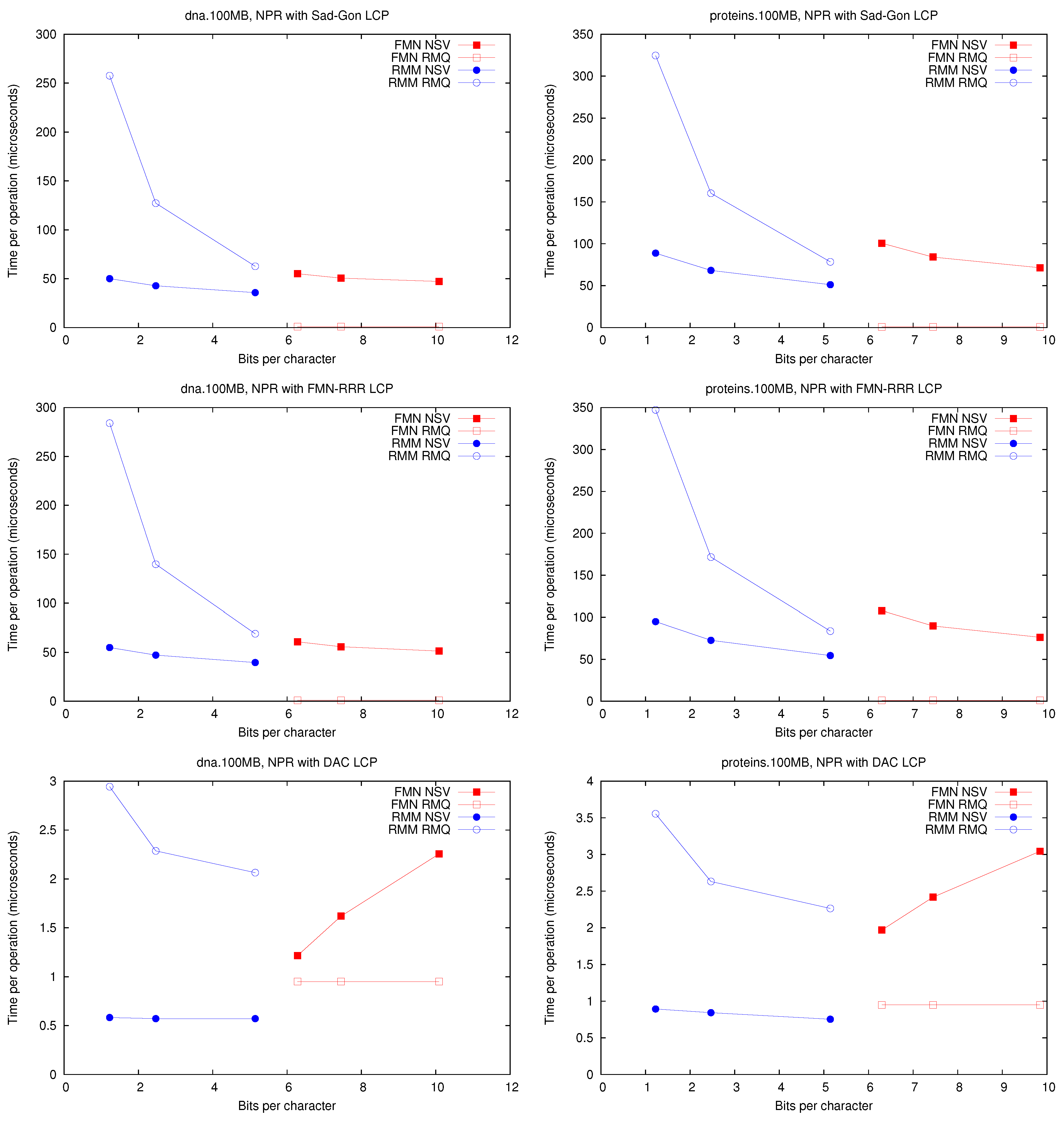
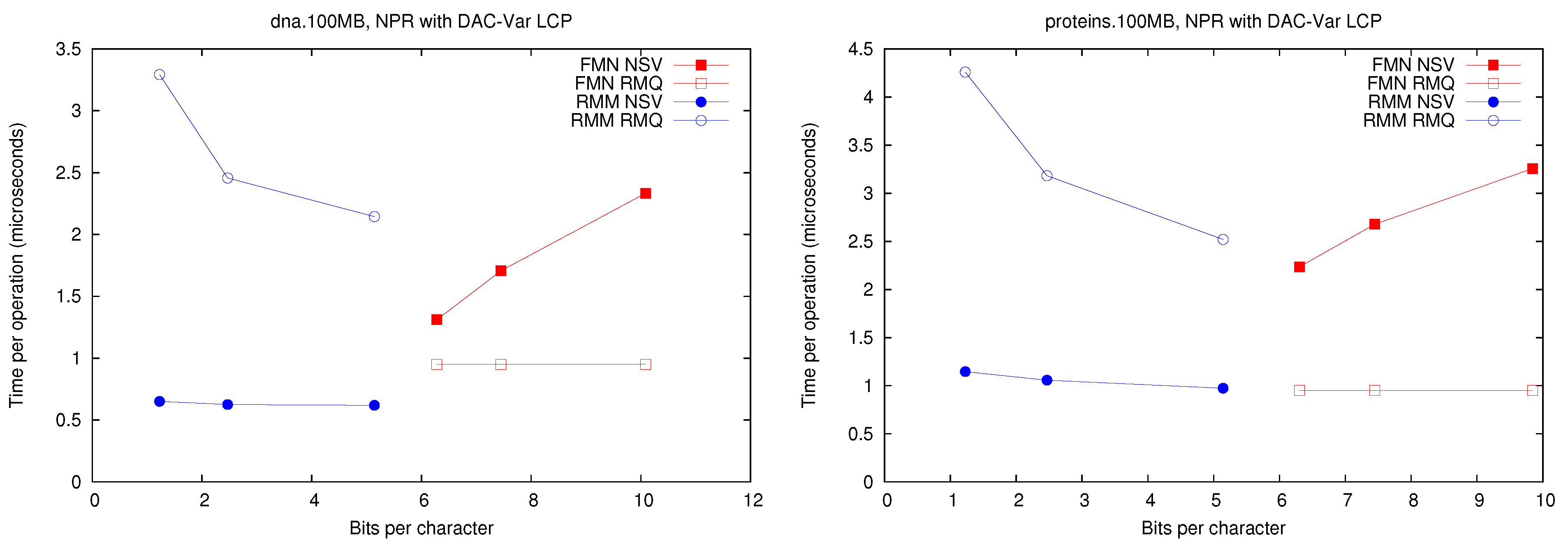
4.2. Experimental Comparison
We tested the performance of the different
implementations by performing 100,000
and
queries at random positions in the
array.
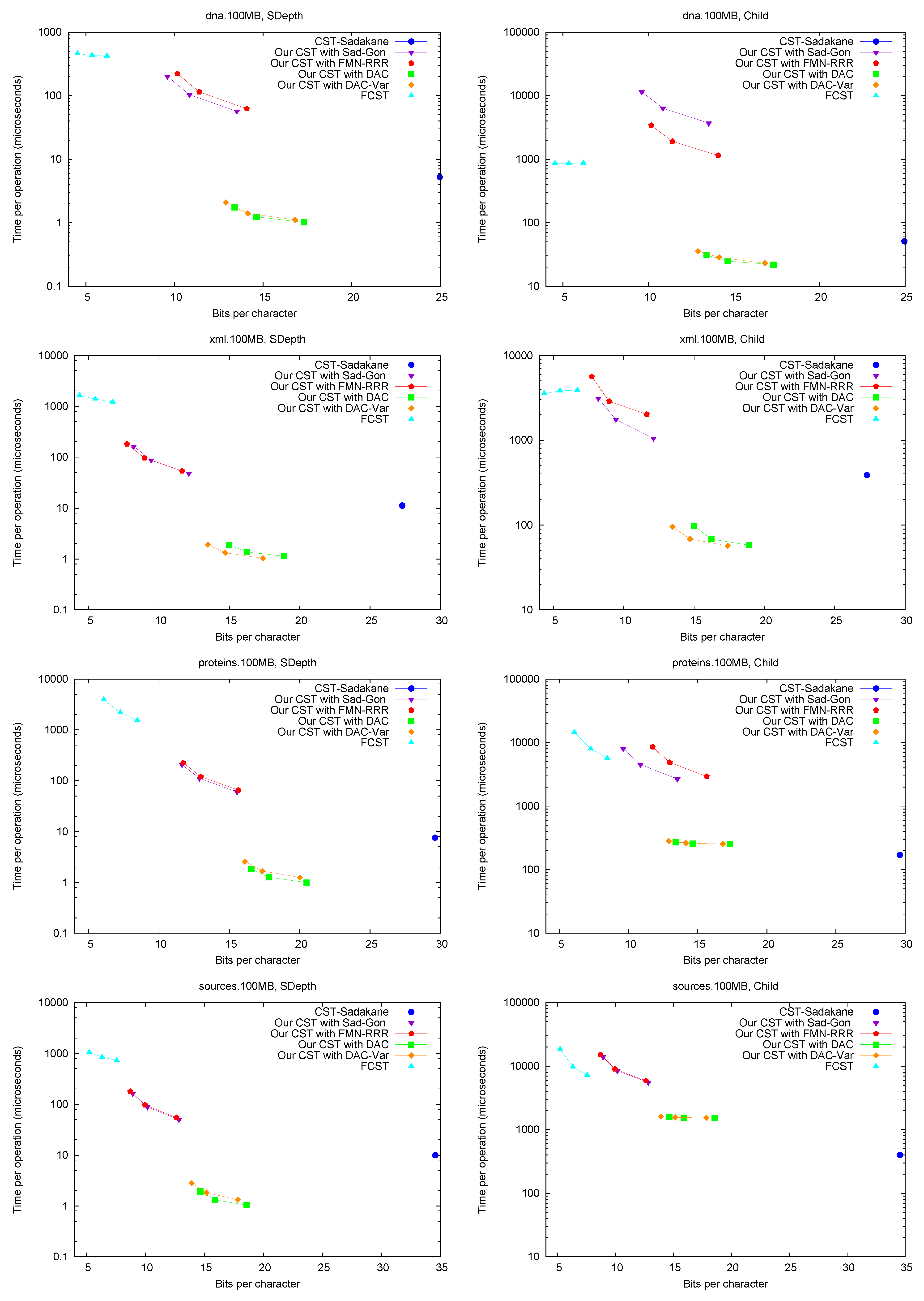
Figure 3 shows the space/time achieved for each implementation on
dna and
proteins (the others texts gave very similar results). We consider the four selected LCP representations, which affect the performance because the algorithms have to access the array. The space we plot is additional to that to store the
array. We obtained space/time tradeoffs by using different block sizes
. Note that
on
does not access
, so the value of
L does not affect it.
Figure 3.
Space/Time for the operations and . Times for are identical to those for .
Figure 3.
Space/Time for the operations and . Times for are identical to those for .
First, it can be seen that performs well using much less space than . In addition, solving (and thus ) with structure is significantly faster than with . This holds under all the representations, regardless that times are one order of magnitude higher with representations and .
On the other hand, is way faster on because it does not need to access at all. It is 2–3 times faster than using or and two orders of magnitude faster than using or . This operation, however, is far less common than and when implementing the CST operations, so its impact is not so high. Another reason to prefer is that it can support a generalized version of and , which allows us to solve operation on suffix trees without adding more memory, as opposed to . In the next section we show how a fully-functional CST can be implemented on top of the representation.
5. Our Compressed Suffix Tree
Our CST implementation applies our
algorithms of
Section 4 on top of some
representation from those chosen in
Section 3. This solves most of the tree traversal operations by using the formulas provided by Fischer
et al. [
18], which we do not repeat here. In some cases, however, we have deviated from the theoretical algorithms for practical considerations.
TDepth: We proceed by brute force using Parent, as there is no practical solution in the theoretical proposal.
NSibling: There is a bug in the original formula [
18] in the case
v is the next-to-last child of its parent. According to them,
first obtains its parent
, then checks whether
(in which case there is no next sibling), then checks whether
(in which case the next sibling is leaf
), and finally answers
, where
. This
is aimed at finding the end of the next sibling of the next sibling, but it fails if we are near the end. Instead, we replace it by the faster
.
generalizes
by finding the next value smaller or equal to
d, and is implemented almost like
using
.
Child: The children are ordered by letter. We need to extract the children sequentially using and , to find the one descending by the correct letter, yet extracting the of each is expensive. Thus we first find all the children sequentially and then binary search the correct letter among them, thus reducing the use of as much as possible.
LAQ: Instead of the slow complex formula given in the original paper, we use (and ): . This is a complex operation we are supporting with extreme simplicity.
LAQ: There is no practical solution in the original proposal. We proceed as follows to achieve the cost of dParent operations, plus some ones, all of which are reasonably cheap. Since , we first try , which is an ancestor of our answer; let . If we are done; else and we try . We compute (which is measured by using operations until reaching ) and iterate until finding the right node.
Table 3 gives a space breakdown for our CST. We give the space in bpc of Sadakane’s CSA, the 4 alternatives we consider for the LCP representation, and the space of our RMM tree (using
for a “slow” variant and
for a “fast” variant). The last column gives the total bpc considering the smallest “slow” (using
or
for
) and the smallest “fast” (using
or
) alternatives.
Table 3.
Space breakdown of our compressed suffix tree.
Table 3.
Space breakdown of our compressed suffix tree.
| Collection | CSA bpc | LCP bpc | RMM bpc | Total bpc |
|---|
| | | | | Slow | Fast | Slow | Fast |
|---|
| dna | | | | | | 1.23 | | | |
| xml | | | | | | 1.23 | | | |
| proteins | | | | | | 1.23 | | | |
| sources | | | | | | 1.23 | | | |
6. Comparing the CST Implementations
We compare the following CST implementations: Välimäki
et al.’s [
20] implementation of Sadakane’s compressed suffix tree [
11] (
CST-Sadakane); Russo’s implementation of Russo
et al.’s “fully-compressed” suffix tree [
14] (
FCST); and our best variants. These are called
Our CST in the plots. Depending on their
representation, they are suffixed with
,
,
, and
. We do not compare some operations like
Root and
Ancestor because they are trivial in all the implementations;
Locate and
Count because they depend only on the underlying CSA (which is mostly orthogonal, thus
Letter is sufficient to study it);
SLink because it is usually better to do
SLink i times; and
and
because they are not implemented in the alternative CSTs (these two are shown only for ours).
We typically show space/time tradeoffs for all the structures, where the space is measured in bpc (recall that these CSTs replace the text, so this is the overall space required). The times are averaged over a number of queries on random nodes. We use four types of node samplings, which make sense in different typical suffix tree traversal scenarios: (a) Collecting the nodes visited over 10,000 traversals from a random leaf to the root (used for Parent, SDepth, and Child operations); (b) Same but keeping only nodes with at least 5 children (for Letter); (c) Collecting the nodes visited over 10,000 traversals from the parent of a random leaf towards the root via suffix links (used for SLink and TDepth); and (d) Taking 10,000 random leaf pairs (for LCA). The standard deviation divided by the average is in the range [0.21, 2.56] for CST-Sadakane, [0.97, 2.68] for FCST, [0.65, 1.78] for Our CST Sad-Gon, [0.64, 2.50] for Our CST , [0.59, 0.75] for Our CST DAC, and [0.63, 0.91] for Our CST . The standard deviation of the estimator is thus at most 1/100th of that.
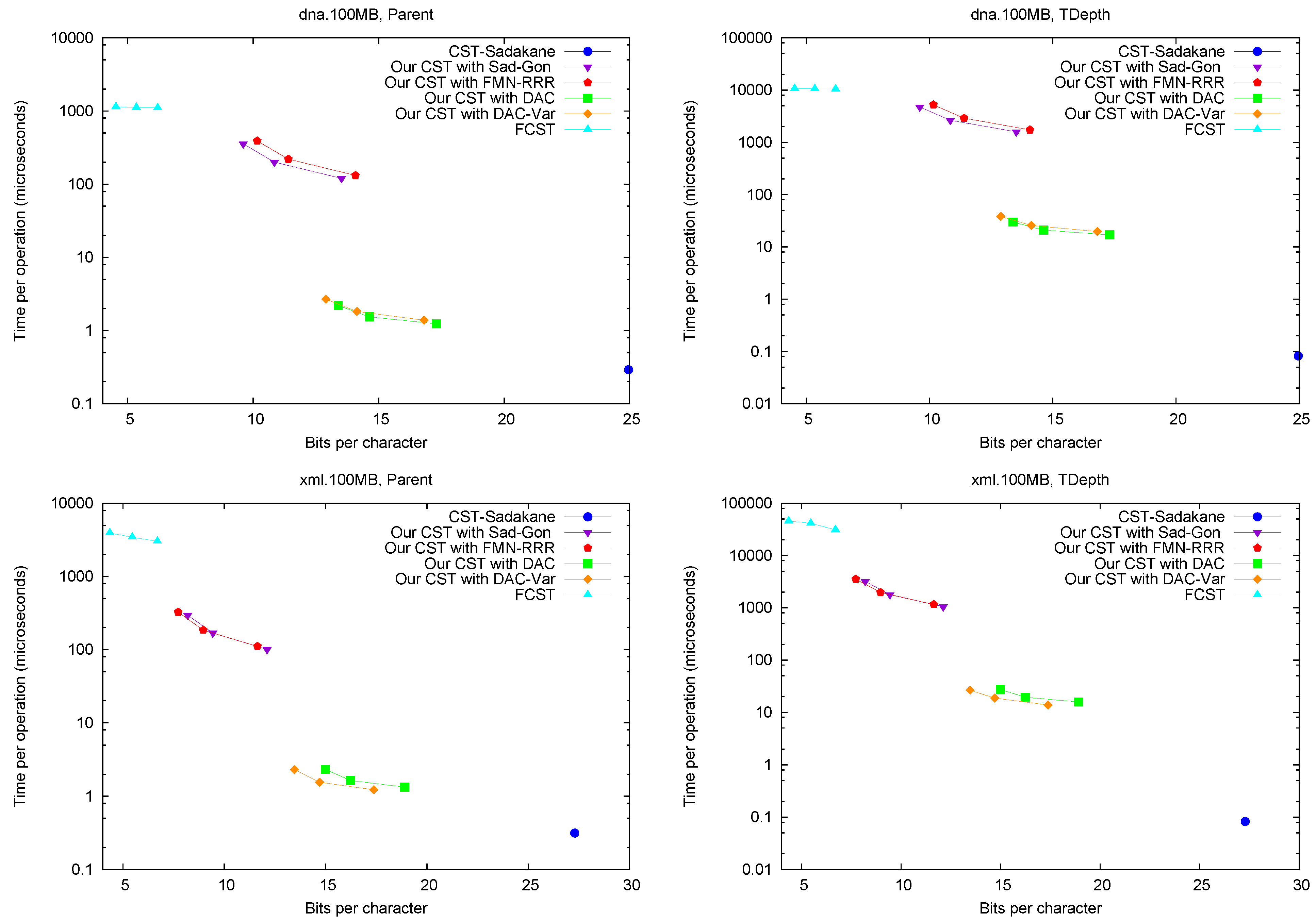
Parent and TDepth.
Figure 4 shows the performance of operations
Parent and
TDepth. As can be seen,
CST-Sadakane is about 5 to 10 times faster than our best results for
Parent and 100 times faster for
TDepth. This is not surprising given that
CST-Sadakane stores the topology explicitly and thus these operations are among the easiest ones. In addition, our implementation computes
TDepth by brute force. Note, on the other hand, that
FCST is about 10 times slower than our slowest implementation.
Figure 4.
Space/Time trade-off performance for operations Parent and TDepth. Note the log scale.
Figure 4.
Space/Time trade-off performance for operations Parent and TDepth. Note the log scale.
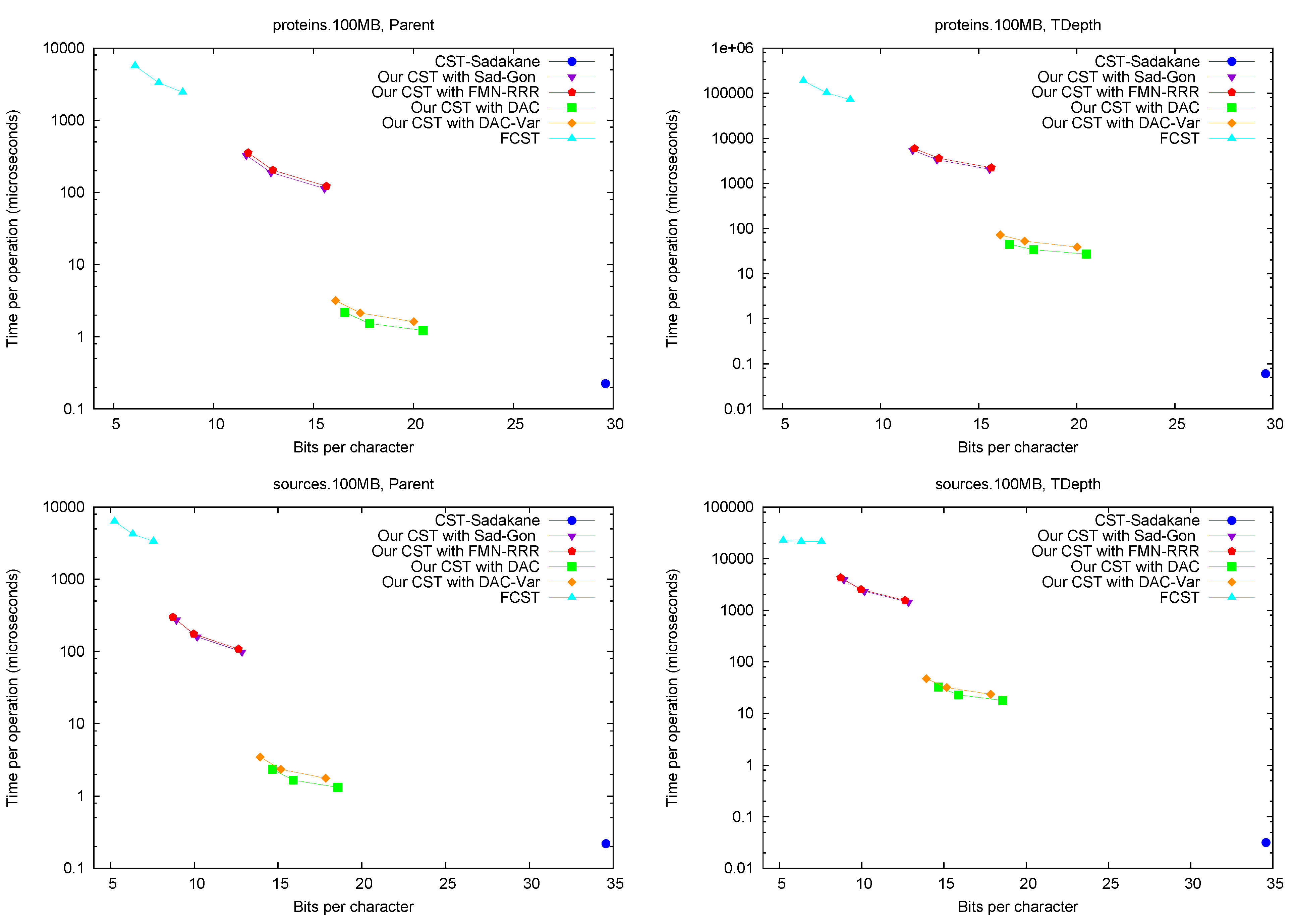
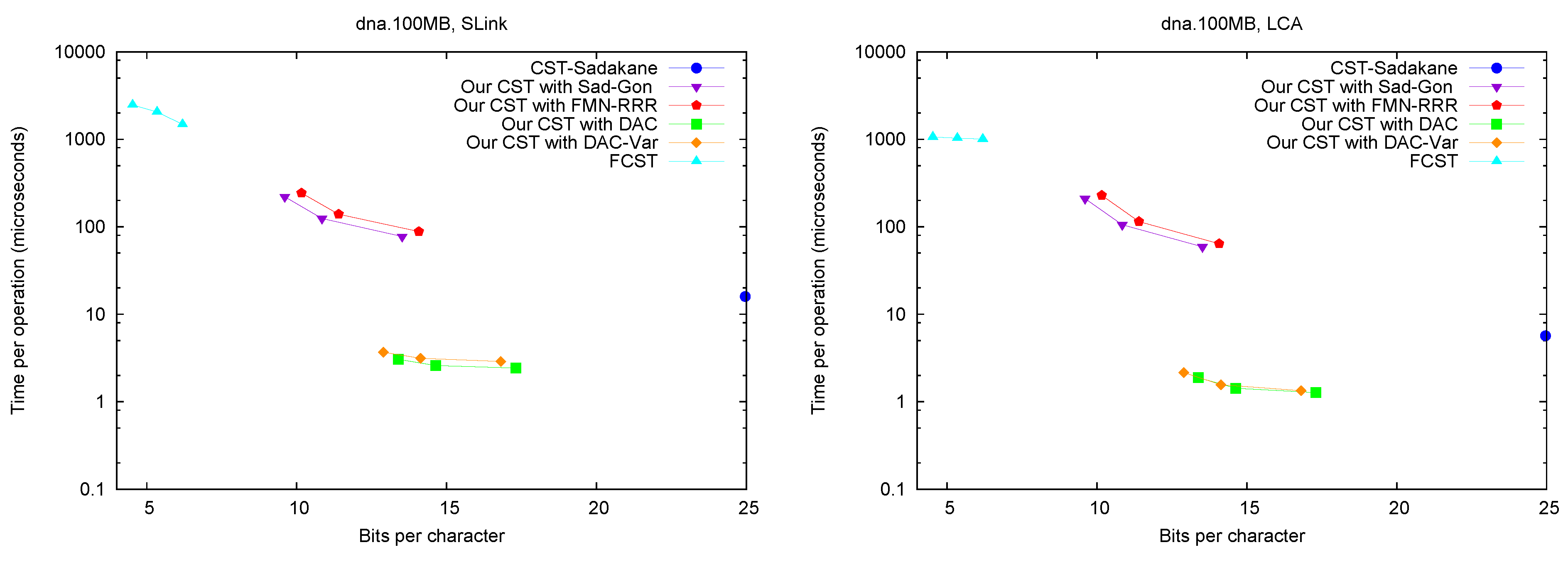
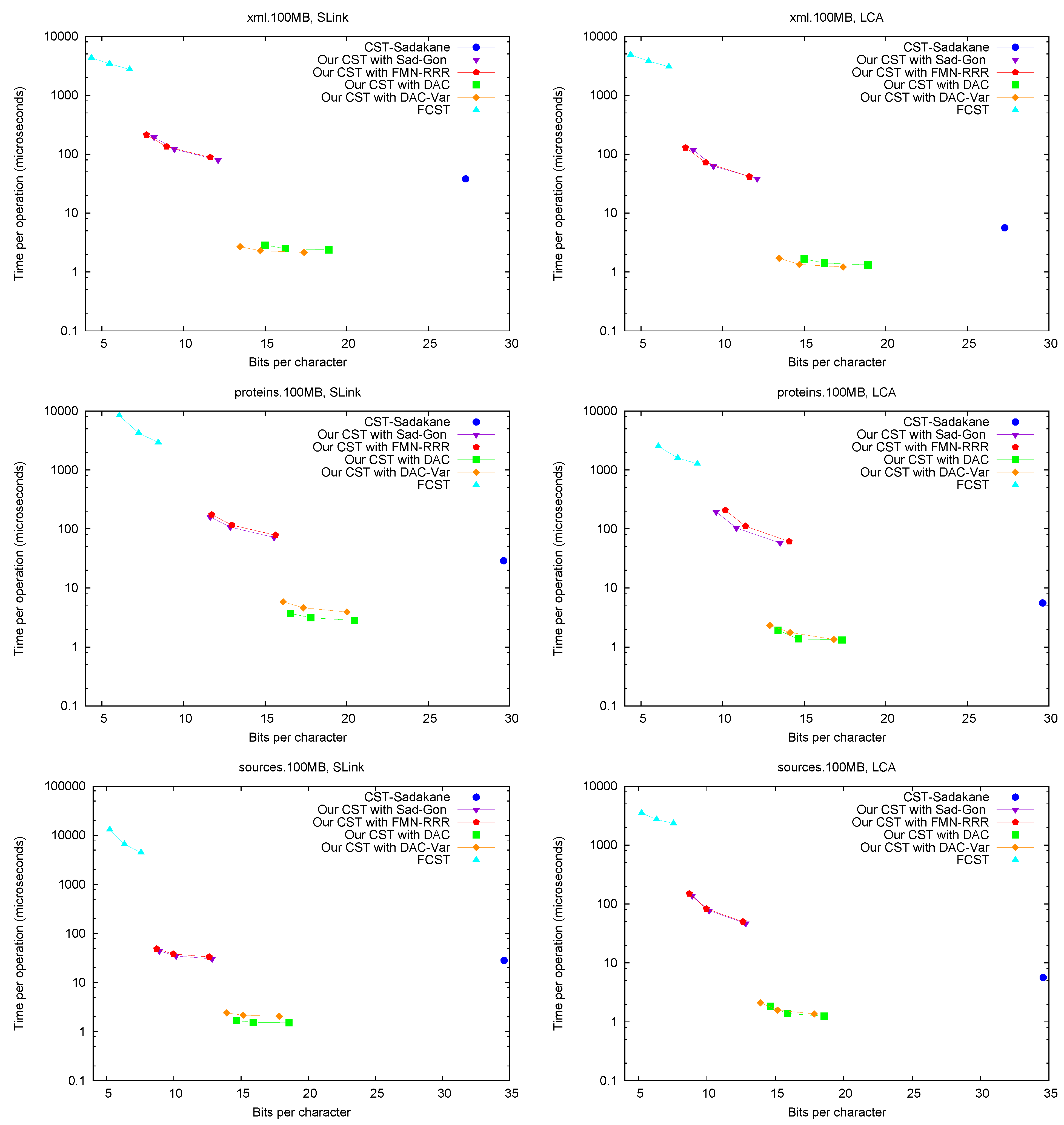
SLink,
LCA,
and SDepth.
Figure 5 shows the performance of operations
SLink and
LCA, which are the ones most specific of suffix trees.
Figure 6 (left) shows operation
SDepth. Those operations happen to be among the most natural ones in Russo’s
FCST, which displays a better performance compared with the previous ones.
CST-Sadakane, instead, is not anymore the fastest. Indeed, our implementations based on
and
are by far the fastest ones for these operations, 10 times faster than
CST-Sadakane and 100 to 1000 times faster than
FCST. Even our slower implementations are way faster than
FCST and close to
CST-Sadakane times.
Figure 5.
Space/Time trade-off performance for operations SLink and LCA. Note the log scale.
Figure 5.
Space/Time trade-off performance for operations SLink and LCA. Note the log scale.
Child. Figure 6 (right) shows operation
Child, where we descend by a random child from the current node. Our times are significantly higher than for other operations, as expected, and the same happens to
CST-Sadakane, which becomes comparable with our “large and fast” variants.
FCST, on the other hand, is not much affected and becomes comparable with our “small and slow” variant. We note that, unlike other operations, the differences in performance depend markedly on the type of text.
Figure 6.
Space/Time trade-off performance for operations SDepth and Child. Note the log scale.
Figure 6.
Space/Time trade-off performance for operations SDepth and Child. Note the log scale.
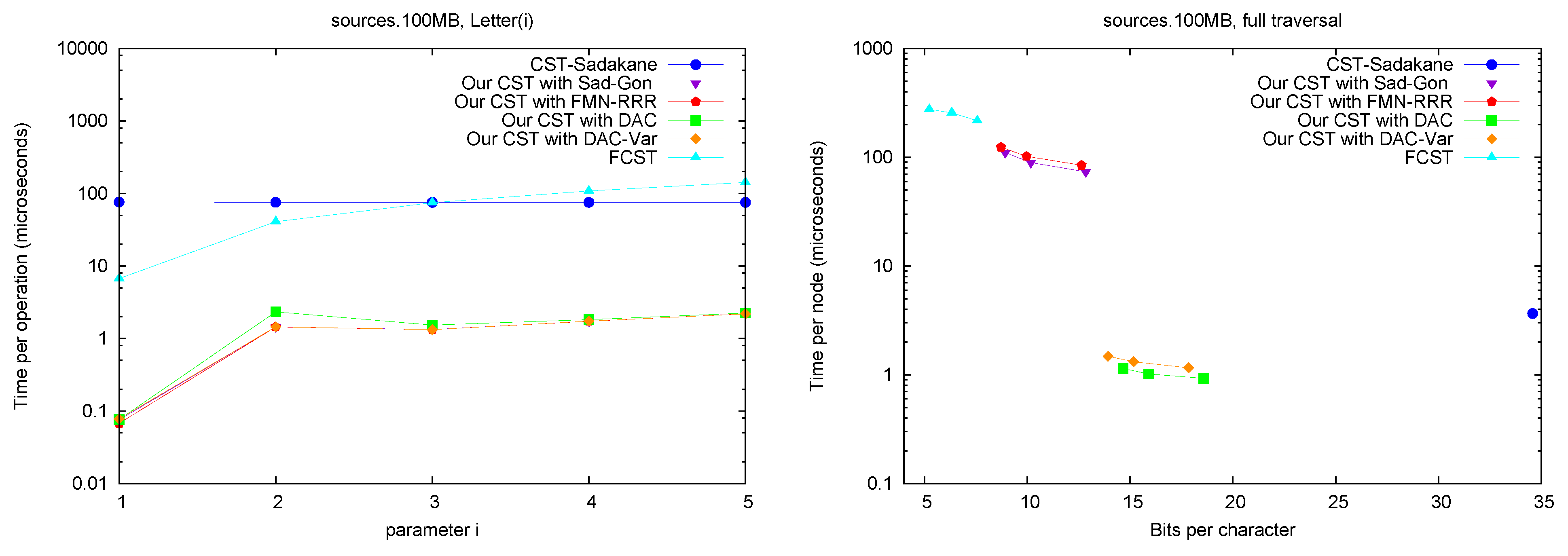
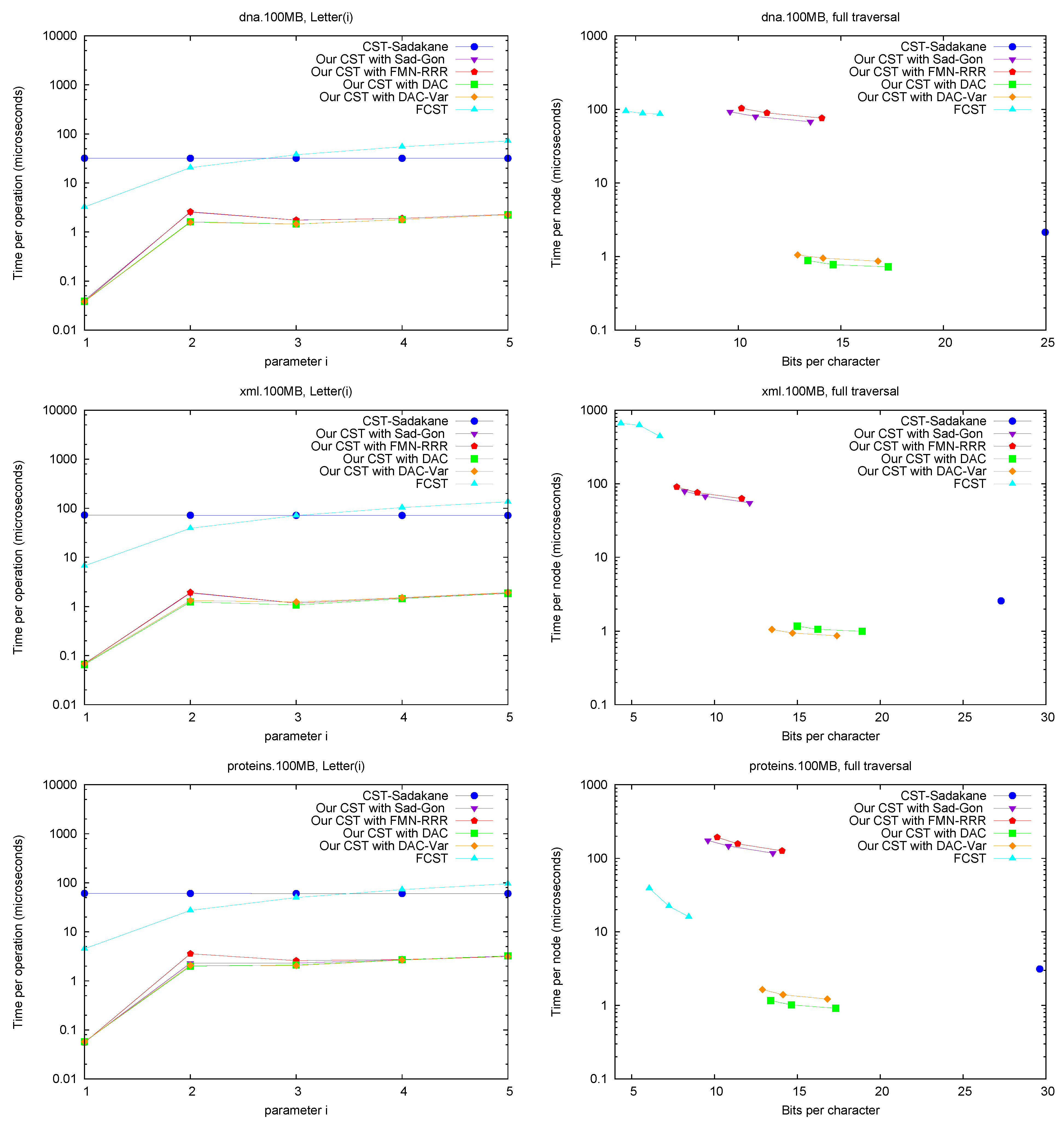
Letter. Figure 7 (left) shows operation
Letter , as a function of
i. This operation depends only on the CSA structure, and requires either applying
times Ψ, or applying once
A and
. The former choice is preferred for
FCST and the latter in
CST-Sadakane. For our CST, using Ψ iteratively was better for these
i values, as the alternative takes around 70 microseconds (recall we use Sadakane’s CSA [
12]).
Figure 7.
Space/Time trade-off performance for operation Letter and for a full tree traversal. Note the log scale.
Figure 7.
Space/Time trade-off performance for operation Letter and for a full tree traversal. Note the log scale.
A full traversal. Figure 7 (right) shows a basic suffix tree traversal algorithm: the classical one to detect the longest repetition in a text. This traverses all of the internal nodes using
FChild and
NSibling and reports the maximum
SDepth. Although
CST-Sadakane takes advantage of locality, our “large and fast” variants are better while using half the space. Our “small and slow” variant, instead, requires a few hundred microseconds, as expected, yet
FCST has a special implementation for full traversals and it is competitive with our slow variant.
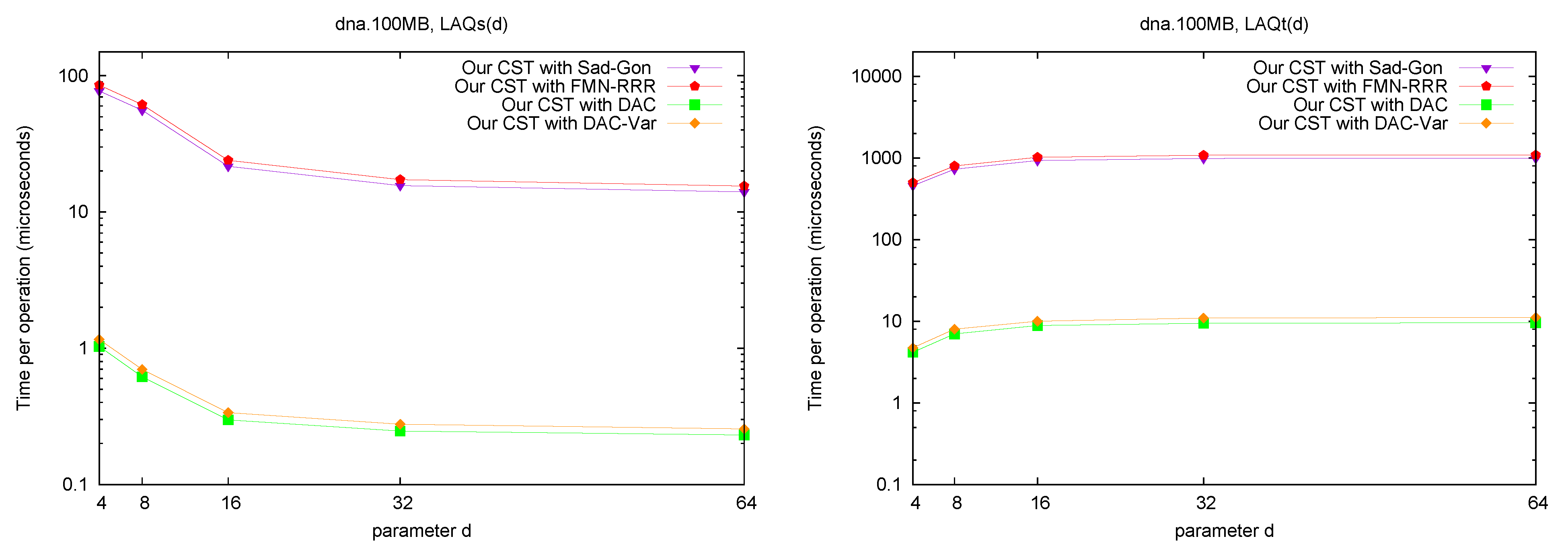
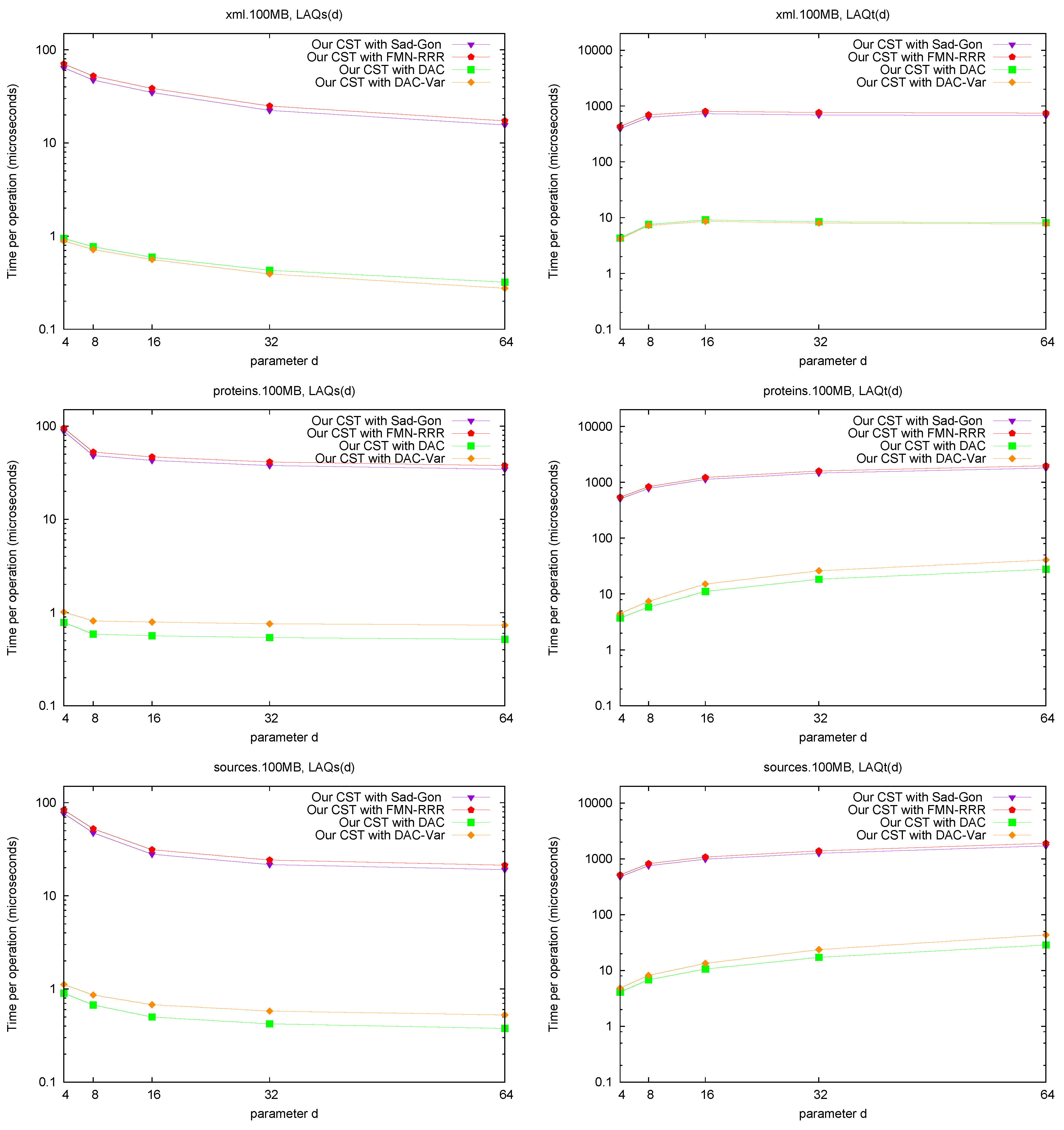
LAQ and LAQ. Figure 8 shows the performance of the operations
and
. The times are presented as a function of parameter
d, where we use
. We query the nodes visited over 10,000 traversals from a random leaf to the root (excluding the root). As expected, the performance of
is similar to that of
Parent, and the performance of
is close to that of doing
Parent d times. Note that, as we increase the value of
d, the times tend to a constant. This is because, as we increase
d, a greater number of queried nodes are themselves the answer to
or
queries.
Figure 8.
Space/Time trade-off performance for operation and . Note the log scale.
Figure 8.
Space/Time trade-off performance for operation and . Note the log scale.
Discussion. The general conclusion is that our CST implementation does offer a relevant tradeoff between the two rather extreme existing variants. Our CSTs can operate within 8–12 bpc (that is, at most 50% larger than the plain byte-based representation of the text, and replacing it) while requiring a few hundred microseconds for most operations (the “small and slow” variants and ); or within 13–16 bpc and carrying out most operations within a few microseconds (the “large and fast” variants /). In contrast, FCST requires only 4–6 bpc (which is, remarkably, as little as half the space required by the plain text representation), but takes the order of milliseconds per operation; and CST-Sadakane takes usually a few tens of microseconds per operation but requires 25–35 bpc, which is close to uncompressed suffix arrays (not to uncompressed suffix trees, though).
We remark that, for many operations, our “fast and large” variant takes half the space of CST-Sadakane and is many times faster. Exceptions are Parent and TDepth, where CST-Sadakane stores the explicit tree topology, and thus takes a fraction of a microsecond. On the other hand, our CST carries out in the same time of Parent, whereas this is much more complicated for the alternatives (they do not even implement it). For Child, where we descend by a random letter from the current node, the times are higher than for other operations, as expected, yet the same happens to all the implementations. We note that FCST is more efficient on operations and SDepth, which are its kernel operations, yet it is still slower than our “small and slow” variant. Finally, TDepth is an operation where all but Sadakane’s CST are relatively slow, yet on most suffix tree algorithms the string depth is much more relevant than the tree depth. Our costs about d times the time of our TDepth.
7. A Repetition-Aware CST
We now develop a variant of our representation that is suitable for highly repetitive text collections, and upgrade it to a fully-functional CST for this case. Recall that we need three components: A CSA, an LCP representation, and fast queries on that sequence.
We use the RLCSA [
25] as the base CSA of our repetition-aware CST. We also use the compressed representation of
(
i.e., bitmap
H) [
18]. Since now we assume
, we use a compressed bitmap representation that is useful for very sparse bitmaps [
24]: We
δ-encode the runs of 0’s between consecutive 1’s, and store absolute pointers to the representation of every
sth 1. This is very efficient in space and solves
queries in time
, which is the operation needed to compute a
value.
The main issue is how to support fast operations using the RLCSA and our LCP representation. Directly using the
tree structure requires at least 1 bpc (see
Figure 3), which is too much when indexing repetitive collections. Our main idea is to replace the regular structure of tree
by the parsing tree obtained by a Re-Pair compression of the sequence
. We now explain this idea in detail.
7.1. Grammar-Compressing the LCP Array
To solve the queries on top of the LCP array, we represent a part of it in grammar-compressed form. This will be redundant with our compressed representation of array H, which was already explained.
Following the idea in Fischer
et al. [
18], we grammar-compress the differential LCP array, defined as
if
, and
. This differential LCP array contains now
areas that are exact repetitions of others, and a Re-Pair-based compression of it yields
words [
18,
35]. We note, however, that the compression achieved in this way is modest [
35]: We guarantee
words, whereas the RLCSA and PLCP representations require basically
bits. Indeed, the poor performance of variant
in
Section 3 shows that the idea should not be applied directly.
To overcome this problem, we take advantage of the fact that this representation is redundant with H. We truncate the parsing tree of the grammar, and use it as a device to speed up computations that would otherwise require expensive accesses to (i.e., to bitmap H).
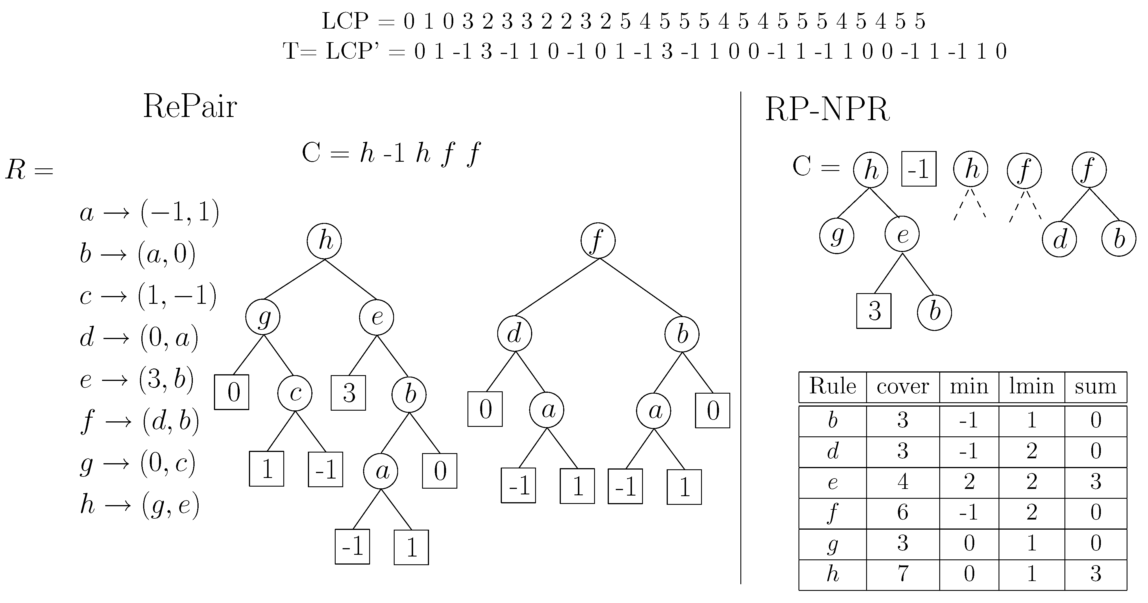
Let
R and
C be the results of compressing
with Re-Pair. Every nonterminal
i of
R expands to a substring
of
. No matter where
S appears in
(indeed, it must appear more than once), we can store some values that are intrinsic to
S. Let us define a relative sequence of values associated to
S, as follows:
and
. Then, we define the following variables associated to the nonterminal:
is the minimum value in .
and are the leftmost and rightmost positions j where , respectively.
is the sum of the values .
is the number of values in .
As most of these values are small, we encode them with DACs [
43], which use less space for short numbers while providing fast access (
is stored as the difference with
).
To reduce space, we prune the grammar by deleting the nonterminals i such that , where t will be a space/time tradeoff parameter. However, “short” nonterminals that are mentioned in sequence C are not deleted.
This ensures that we can skip
symbols of
with a single access to the corresponding nonterminal in
C, except for the short nonterminals (and terminals) that are retained in
C. To speed up traversals on
C, we join together maximal consecutive subsequences of nonterminals and terminals in
C that sum up a total
: We create a new nonterminal rule in
R (for which we precompute the variables above) and replace it in
C, deleting those nonterminals that formed the new rule and do not appear anymore in
C. This will also guarantee that no more than
accesses to
are needed to solve queries. Note that we could have built a hierarchy of new nonterminals by recursively grouping
t consecutive symbols of
C, achieving logarithmic operation times just as with tree
[
29], but this turned out to be counterproductive in practice.
Figure 9 gives an example.
Figure 9.
On the left, example of the Re-Pair compression of a sequence . We show R in array form and also in tree form. On the right, our construction over T, pruning with . We show how deep can the symbols of C be expanded after the pruning.
Figure 9.
On the left, example of the Re-Pair compression of a sequence . We show R in array form and also in tree form. On the right, our construction over T, pruning with . We show how deep can the symbols of C be expanded after the pruning.
Finally, sampled pointers are stored to every
c-th cell of
C. Each sample for position
, stores:
, that is, the first position corresponding to .
, that is, the value .
7.2. Computing NSV, PSV, and RMQ
To answer , we first look for the rule that contains : We binary search for the largest such that and then sequentially advance on until finding the largest j such that . At the same time, we compute .
Now, if , it is possible that is within the same . In this case, we search recursively the tree expansion with root for the leftmost value to the right of i and smaller than : Let in the grammar. We recursively visit child a if and . If we find no answer there, or we had decided not to visit a, then we set and and recursively visit child b if . Note that if we do not need to enter b, but can simply use the value and the position for the minimum. If we also find no answer inside b, or we had decided not to visit b, we return with no value. On the other hand, if we reach a leaf l during the recursion, we sequentially scan the array , updating and increasing . If at some position we find a value smaller than , we report the position .
If we return with no value from the first recursive call at , it was because the only values smaller than were to the left of i. In this case, or if we had decided not to enter into because , we sequentially scan , while updating and , until finding the first k such that . Once we find such k, we are sure that the answer is inside . Thus we enter into with a procedure very similar to the one for (albeit slightly simpler as we know that all the positions are larger than i). In this case, as the LCP values are discrete, we know that if , there is no smaller value to the left of the value, so in this case we directly answer the corresponding value, without accessing the array. The solution to is symmetric.
To answer , we find the rules and containing x and y, respectively. We sequentially scan and store the smallest value found (in case of ties, the leftmost). If the minimum is smaller than the corresponding values and , we directly return the value corresponding to position . Else, if the global minimum in is equal to or less than the minimum for , we must examine to find the smallest value to the right of . Assume . We recursively enter into a if , otherwise we skip it. Then, we update and , and enter into b if , otherwise we directly consider as a candidate for the minimum sought. Finally, if we arrive at a leaf we scan it, updating ℓ and , and consider all the values ℓ where as candidates to the minimum. The minimum for is the smallest among all candidates to minimum considered, and with or the leaf scanning process we know its global position. This new minimum is compared with the minimum of for . Symmetrically, in case contains a value smaller than the minimum for , we have to examine for the smallest value to the left of .
7.3. Analysis
For the analysis we will assume that we hierarchically group the terminals and nonterminals of consecutive symbols in
C (by extending the grammar) using a grouping factor of
g, although, as explained, it turned out to be faster in practice not to do so. We will call
h the height of the grammar, which can be made
by generating balanced grammars [
48] (we experiment with balanced and unbalanced grammars in the next section). We also use sampling steps
c to access
C and
s for the
representation. We also assume
s is the sampling step of the RLCSA, thus accessing one
cell takes
time.
Let us first consider operation (and ). We spend time to binary search and move from to . If we have to expand , the cost increases by : Note that if we had entered a, and obtained no answer inside it, then we can directly use and thus do not enter b, so we only enter one of the two. At the leaf of the grammar tree of , we may scan symbols of using , which costs . Further, the scanning of takes time assuming the hierarchical grouping, and the final expansion of takes again time.
Now consider operation . Again, we spend time to find and , and then expand them as before: Only one of the two branches is expanded in each case, so the time is . Finally, we need time to traverse the area .
Thus, for all the operations, the cost is .
Let , and recall that r is the number of runs, so if using Re-Pair. The sampling parameters involve bits for the sampling of C, plus for the sampling of , plus for the sampling of the RLCSA, plus for the new rules created in the hierarchy for C. Parameter t involves in practice an important reduction in , the set of rules, but this cannot be upper bounded in the worst case unless the grammar is balanced, in which case it is reduced to rules.
By choosing , , , and assuming a balanced grammar, the cost of the operations simplifies to and the extra space incurred by the samplings is bits. This can be reduced to any , for any constant k, by raising the time complexity to .
8. Experimental Evaluation on Repetitive Collections
We used various DNA collections from the Repetitive Corpus of
Pizza & Chili [
49]. We took DNA collections
Influenza and
Para, which are the most repetitive ones, and
Escherichia, a less repetitive one. These are collections of genomes of various bacteria of those species. We also use
Plain DNA, which is plain DNA from
PizzaChili, as a non-repetitive baseline. On the other hand, in order to show how results scale with repetitiveness, we also included
Einstein, corresponding to the Wikipedia versions of the article about Einstein in German, although it is not a biological collection.
Table 4 (left) gives some basic information on the collections, including the number of runs in Ψ (much lower than those for general sequences; see
Table 2).
For the RLCSA we used a fixed sampling that gave reasonable performance: One absolute value out of 32 is stored to access , and one text position every 128 is sampled to compute . Similarly, we used sampling step 32 for the δ-encoding of the bitmaps Z and O that encode H.
Table 4.
Text size and size of our CST (which replaces the text), both in MB, and number of runs in Ψ. On the right, bpc for the different components, and total bpc of the different collections considered. The NPR structure is the smallest setting between and for that particular text.
Table 4.
Text size and size of our CST (which replaces the text), both in MB, and number of runs in Ψ. On the right, bpc for the different components, and total bpc of the different collections considered. The NPR structure is the smallest setting between and for that particular text.
| Collection | Text Size | Runs (
) | CST size | RLCSA | (P)LCP | NPR | Total |
|---|
| Influenza | 148 | 0.019 | 27 | 0.77 | 0.21 | 0.42 | 1.40 |
| Para | 410 | 0.036 | 67 | 1.28 | 0.26 | 0.36 | 1.90 |
| Escherichia | 108 | 0.134 | 48 | 2.46 | 0.92 | 0.39 | 3.77 |
| Plain DNA | 50 | 0.632 | 61 | 5.91 | 3.62 | 0.29 | 9.82 |
| Einstein | 89 | 0.001 | 3 | 0.48 | 0.01 | 0.14 | 0.63 |
Table 4 (right) shows the resulting sizes. The bpc of the CST is partitioned into those for the RLCSA, for the PLCP (
H), and for NPR, which stands for the data structure that solves
queries. For the latter we used
, which offered answers within 2 milliseconds (ms). Note that Fischer
et al.’s [
18] compression of bitmap
H does work in repetitive sequences, unlike what happened in the general case: We reduce the space from 2 bpc to 0.21–0.26 bpc on the more repetitive DNA sequences, for example. Similarly, the regular RMM-tree uses 1–5 bpc, whereas our version adapted to repetitive sequences uses as little as 0.3–0.4 bpc. The good space performance of the RLCSA, compared with a regular CSA for general sequences, also contributes to obtain a remarkable final space of 1.4–1.9 bpc for the more repetitive DNA sequences. This value deteriorates until approaching, for plain (non-repetitive) DNA, the same 10 bpc that we obtained before. Thus our data structure adapts smoothly to the repetitiveness (or lack of it) of the collection.
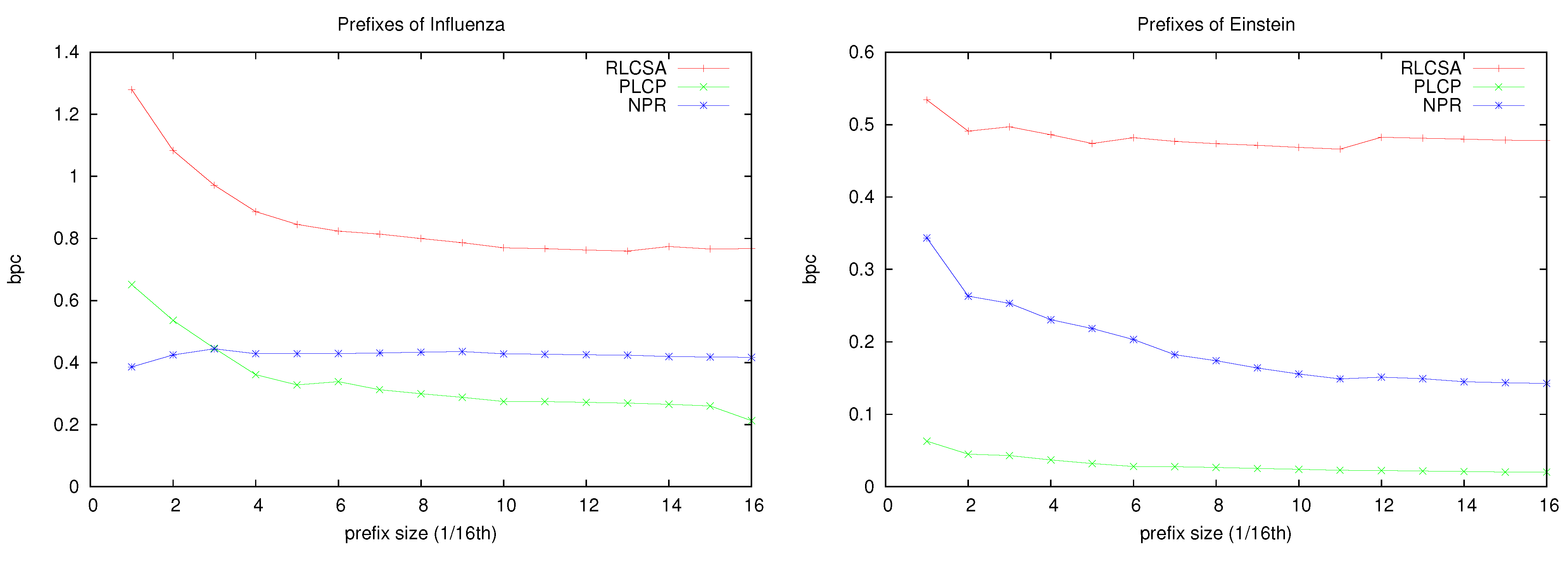
On the other hand, on Einstein, which is much more repetitive, the total space gets as low as 0.6 bpc. This is a good indication of what we can expect on future databases with thousands of individuals of the same species, as opposed to these testbeds with a few tens of individuals, or with more genetic variation. To give more insight into how the space of our structures evolve as the repetitiveness increases,
Figure 10 shows the space used by each component of the index on increasing prefixes of collections
Influenza and
Einstein. It can be seen that, as the we index more of the collection, the space of the different components decreases until reaching a stable point that depends on the intrinsic repetitiveness of the collection (this is reached earlier for
Influenza). Note, however, that even in the more repetitive
Einstein, the RLCSA stabilizes very early at a fixed space. This space is that of the suffix array sampling, which is related to the speed of computing the contents of suffix array cells (and hence computing LCP values). It is interesting that Mäkinen
et al. [
25] proposed a solution to compress this array that proved impractical for the small databases we are experimenting with, but whose asymptotic properties ensure that will become practical for sufficiently large and repetitive collections.
Figure 10.
Evolution of the space, in bpc, of our structures for increasing prefixes of collections Influenza and Einstein.
Figure 10.
Evolution of the space, in bpc, of our structures for increasing prefixes of collections Influenza and Einstein.
Let us discuss the NPR operations now. We used a public Re-Pair compressor built by ourselves [
50], which offers two alternatives when dealing with symbols of the same frequencies. The basic one, which we will call
, stacks the pairs of the same frequency, whereas the second one,
, enqueues them and obtains much more balanced grammars in practice. For our structure we tested values
. We also include the basic regular RMM-tree of the previous sections (but running over our RLCSA and PLCP representations), to show that on repetitive collections our grammar-based version offers better space/time tradeoffs than the regular tree
. For this version,
, we used values
.
We measure the times of operations
(as
is symmetric) and
following the methodology of
Section 6: We choose 10,000 random suffix tree leaves (corresponding to uniformly random suffix array intervals
) and navigate towards the root using operation
. At each such node, we also measure the string depth,
. We average the times of the
and
queries involved.
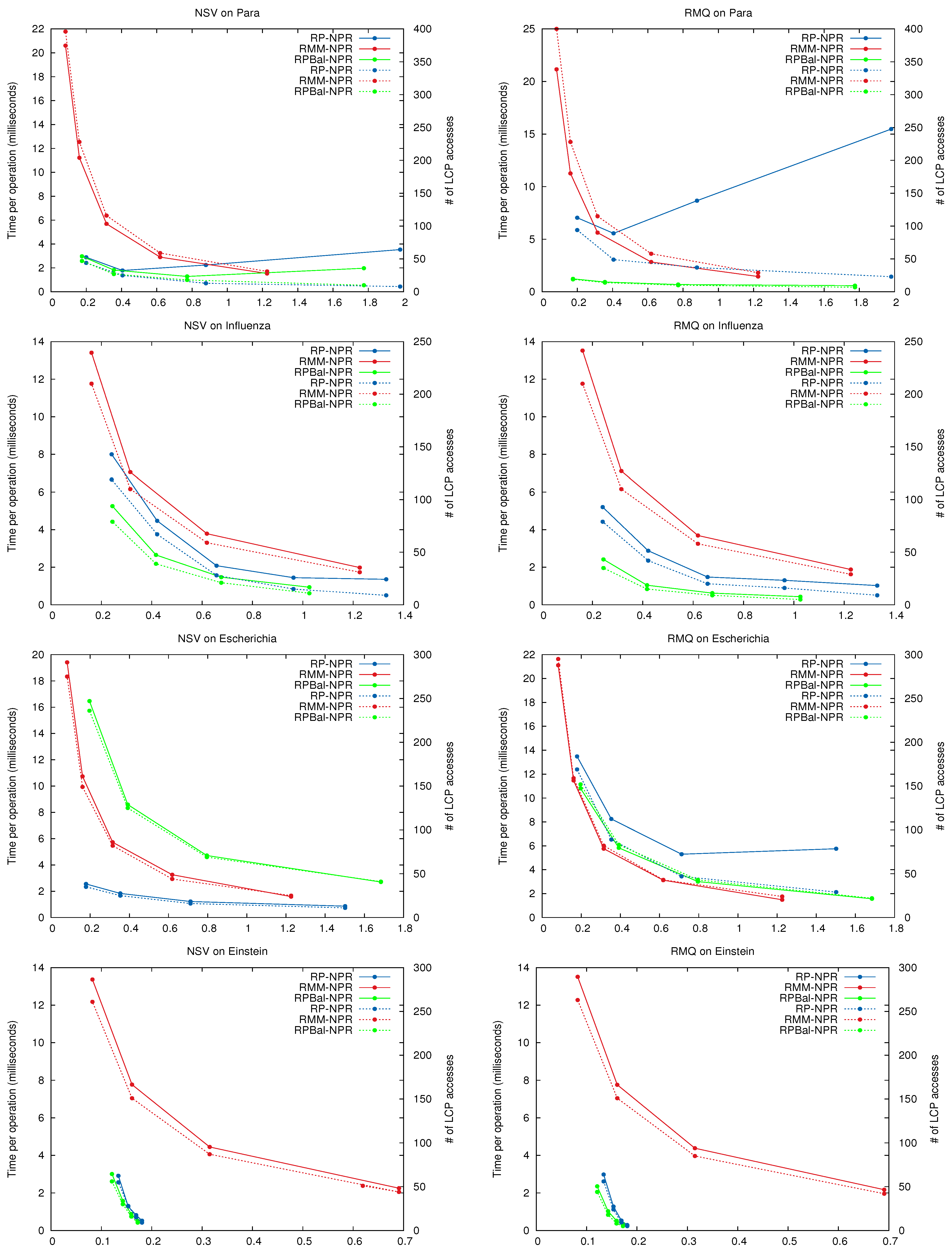
Figure 11 shows the space/time performance of
,
, and
on the repetitive collections. In addition, it shows the number of explicit accesses to
made per NPR operation.
In general the curves for total time and number of accesses have the same shape, showing that in practice the main cost of the NPR operations lies in retrieving the LCP values. In some cases, and most noticeably for queries on Para using , using more space yields fewer accesses but higher time. This is because the Re-Pair grammars may be very unbalanced, and giving more space to them results in less tree pruning. Thus deeper trees, whose nodes have to be traversed one by one to cover short passages, are generated. largely corrects this effect by generating more balanced grammar trees.
Clearly, and dominate the space/time map for all queries. They always make better use of the space than the regular tree of . is usually better than , except on some particular cases, like on Escherichia, where is faster.
Figure 11.
Space/Time performance of NPR operations. The x-axis shows the size of the NPR structure. On the left y-axis the average time per operation (solid lines), and on the right y-axis the average number of LCP accesses per operation (dashed lines). Note the log scale on y for Einstein.
Figure 11.
Space/Time performance of NPR operations. The x-axis shows the size of the NPR structure. On the left y-axis the average time per operation (solid lines), and on the right y-axis the average number of LCP accesses per operation (dashed lines). Note the log scale on y for Einstein.
The times of our best variants are in the range of a few milliseconds per operation. This is high compared with the times obtained on general sequences. The closest comparison point is Russo
et al.’s CST [
14] whose times are very similar, but it uses 4–6 bpc compared with our 1.4–1.9 bpc. As discussed, we can expect our bpc value to decrease even more on larger databases. Such a representation, even if taking milliseconds per operation, is very convenient if it saves us from using a disk-based suffix tree. Note also that, on very repetitive collections, we could avoid pruning the grammar at all. In this case the grammar itself would give access to the LCP array much faster than by accessing bitmap
H.

