Monitoring Threshold Functions over Distributed Data Streams with Node Dependent Constraints

Abstract

Monitoring data streams in a distributed system has attracted considerable interest in recent years. The task of feature selection (e.g., by monitoring the information gain of various features) requires a very high communication overhead when addressed using straightforward centralized algorithms. While most of the existing algorithms deal with monitoring simple aggregated values such as frequency of occurrence of stream items, motivated by recent contributions based on geometric ideas we present an alternative approach. The proposed approach enables monitoring values of an arbitrary threshold function over distributed data streams through stream dependent constraints applied separately on each stream. We report numerical experiments on a real-world data that detect instances where communication between nodes is required, and compare the approach and the results to those recently reported in the literature.

1. Introduction

In many emerging applications one needs to process a continuous stream of data in real time. Sensor networks [1], network monitoring [2], and real-time analysis of financial data [3,4] are examples of such applications. Monitoring queries is a particular class of queries in the context of data streams. Previous work in this area deals with monitoring simple aggregates [2], or term frequency occurrence in a set of distributed streams [5].

A general framework for efficient local algorithms monitoring l₂ norm of the data average of large networks of computers, wireless sensors, or mobile devices was introduced in [6], and further developed in [7]. The current contribution is motivated by results recently reported in [8,9] with focus on a special case of the general model considered in [7]. This special case can be briefly described as follows:

Let be a set of data streams collected at n nodes. Let v₁(t),...,v_n(t) be d dimensional real time varying vectors derived from the streams. For a function we would like to confirm the inequality

(1)

while minimizing communication between the nodes. Monitoring inequality (1), or monitoring geometric location of the mean is a problem that can be addressed using a variety of different mathematical tools. A specific choice of a monitoring tool is up to the user. We note that the problem as stated above does not specify any particular tool, l₂, or any other norm that is required to address it.

The problem was recently addressed in [10], where the approach proposed imposes equal constraints on each node. In addition to previously used l₂ norm (see, e.g., [6,7,8,9,11]) the paper provides theoretical framework for using a wide variety of convex functions, and, as an illustration, runs numerical experiments using l₂, l₁ and l_∞ norms. In all numerical experiments reported in [10] an application of the same algorithm with l₁ norm generates superior results. This paper extends results in [10] in a machine learning direction—a constraint imposed on each node depends on the stream history at the node.

As a simple illustration of the problem considered in the paper we focus on two scalar functions v₁(t) and v₂(t), and the identity function f (i.e., f(x) = x).We would like to guarantee the inequality

while keeping the nodes silent as much as possible. A possible strategy is to verify the initial inequality and to keep both nodes silent while

The first time t₁ when one of the functions, say v₁(t), crosses the boundary of the local constraint, i.e., the nodes communicate, the mean v(t₁) is computed, the local constraint δ is updated and made available to the nodes, and nodes are kept silent as long as the inequalities hold.

The main contributions of this paper are listed next. We demonstrate that:

• 1. This approach works for a non-linear monitoring function f.
• 2. The results depend on the choice of a norm, and the numerical results reported show that l₂ is probably not the best norm when one aims to minimize communication between nodes. In addition to the numerical results presented we also provide a simple illustrative example that highlights this point (see Remark 4.2).
• 3. Selection of node dependent local constraints may decrease communication between the nodes.
• 4. The approach suggested in [10] and adopted in this paper paves the way to achieve further communication savings by clustering nodes, and monitoring cluster coordinators. Although this research direction is beyond the scope of this paper we address it briefly in Section 6.

In the next section we provide a text mining related example that leads to a non-linear threshold function f.

2. Text Mining Application

Let T be a finite text collection (for example a collection of mail or news items). We denote the size of the set T by |T|. We will be concerned with two subsets of T:

• 1. R–the set of “relevant" texts (text not labeled as spam),
• 2. F–the set of texts that contain a “feature" (word or term for example).

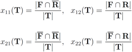
We denote complements of the sets by respectably (i.e., ), and consider the relative size of the four sets as follows:

(2)

Note that

The function f is defined on the simplex (i.e., , ), and given by

(3)

where throughout the paper. We next relate empirical version of information gain Equation (3) and the information gain (see e.g., [12]).

Let Y and X be random variable with know distributions

Entropy of Y is defined by

(4)

Entropy of Y conditional on X = x denoted by is defined by

(5)

Conditional entropy and information gain are given by

(6)

Information gain is symmetric, indeed

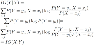
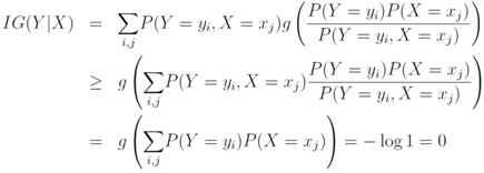
Due to convexity of , information gain is non-negative

It is easy to see that Equation (3) provides information gain for the “feature".

As an example, we consider n agents installed on n different servers and a stream of texts arriving at the servers. Let be the last w texts received at the server, with . Note that

i.e., entries of the global contingency table are the average of the local contingency tables .

For the given “feature" and a predefined positive threshold r we would like to verify the inequality

while minimizing communication between the servers. Note that Equation (3) is a nonlinear function. The case of a nonlinear monitoring function is different from that of linear one (in fact [8] calls the nonlinear monitoring function case “fundamentally different"). In the next section we demonstrate the difference, and describe an efficient way to handle the nonlinear case.

3. Non-Linear Threshold Function: An Example

We start with a slight modification of a simple one dimensional example presented in [8].

Example 3.1Let , and , are scalar values stored at two distinct nodes. Note that if , and , then

If , and , then

Finally, when , and one has

(7)

The simple illustrative example leads the authors of [8] to conclude that it is impossible to determine from the values of f at the nodes whether its value at the average is above the threshold or not. The remedy proposed is to consider the vectors and to monitor the values of f on the convex hull conv instead of the value of f at the average Equation (1). This strategy leads to sufficient conditions for Equation (1), and may be conservative.

The monitoring techniques for values of f on conv without communication between the nodes are based on the following two observations:

• 1. Convexity property. The mean v(t) is given by , i.e., the mean v(t) is in the convex hull of , and is available to node j without much communication with other nodes.
• 2. If is an l₂ ball of radius centered at , then

(8)

(see Figure 1). Since each ball

(9)

can be monitored by node j with no communication with other nodes, Equation (8) allows to split monitoring of conv into n independent tasks executed by the n nodes separately and without communication.

Figure 1. ball cover.

Figure 1. ball cover.

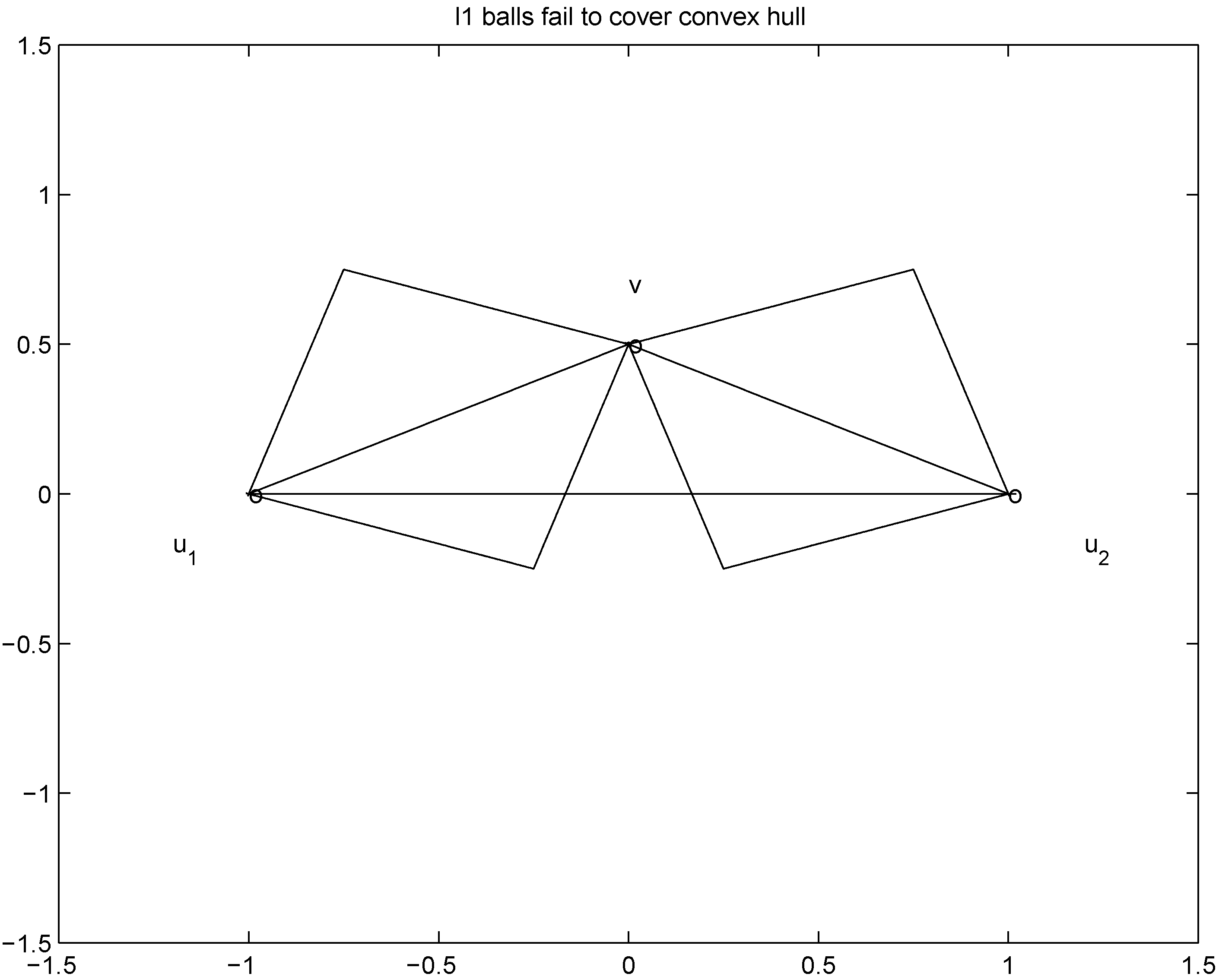
While the inclusion Equation (8) holds when is substituted by with as we show later (see Remark 4.3) the inclusion fails when, for example, (for experimental results obtained with different norms see Section 5).

In this paper we propose an alternative strategy that will be briefly explained next using Example 3.1, , and assignment provided by Equation (7). Let δ be a positive number. Consider two intervals of radius δ centered at and , i.e., we are interested in the intervals

If , , and δ is small, then the average is not far from , and is not far from 7 (hence positive). In fact the sum of the intervals is the interval , and

The “zero" points of f are -3 and 3, and as soon as δ is large enough so that the interval “hits" a point where f vanishes, communication between the nodes is required in order to verify Equation (1). In this particular example as long as , and, therefore,

(10)

no communication is required between the nodes.

The condition presented above is a sufficient condition that guarantees Equation (1). As any sufficient condition is, this condition can be conservative. In fact when the distance is provided by the l₂ norm, this sufficient condition is more conservative than the one provided by “ball monitoring" Equation (9) suggested in [8]. On the other hand, since only a scalar δ should be communicated to each node, the value of the updated mean should not be transmitted (hence communication savings are possible), and there is no need to compute the distance from the center of each ball , , to the zero set . For detailed comparison of results we refer the reader to [10].

We conclude the section by remarking that when inequality Equation (1) is reversed the same technique can be used to monitor the reversed inequality while minimizing communication between the nodes. We provide additional details in Section 5. In the next section we extend the above “monitoring with no communication" argument to the general vector setting. The approach suggested in the next section is motivated by an earlier research on robust stability of control systems (see e.g., [13]).

4. Convex Minimization Problem

In this section we state the monitoring problem as a convex minimization problem. For an appropriate analysis background we refer the interested reader to the classical monograph [14]. For the relevant convex analysis material see [15].

Consider the following optimization problem:

Problem 4.1For a function concave with respect to the first d variables and convex with respect to the last nd variables , solve

(11)

A solution for Problem 4.1 with appropriately selected concludes the section.

The connection between Problem 4.1, and the monitoring problem is explained next. Let B be a matrix made of n blocks, where each block is the identity matrix multiplied by , so that for a set of n vectors in one has

(12)

Assume that inequality Equation (1) holds for the vector w, i.e., . We are looking for a vector x “nearest" to w so that , i.e., for some (where is the zero set of f, i.e., ). We now fix z and denote the distance from w to the set . Note that for each y inside the ball of radius centered at w, one has . If y belongs to a ball of radius centered at w, then the inequality holds true.

Let be a “norm" on (specific functions F we run the numerical experiments with will be described later). The nearest “bad" vector problem described above is the following.

Problem 4.2For identify

(13)

We note that Equation (13) is equivalent to The function

is concave (actually linear) in λ, and convex in x. Hence (see e.g., [15])

The right hand side of the above equality can be conveniently written as follows

The conjugate of a function is defined by (see e.g., [15]). We note that

hence to compute

one has to deal with

For many functions g the conjugate can be easily computed. Next we list conjugate functions for the most popular norms

1.

2.

3.

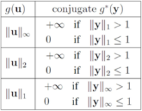
We note that some of the functions F we consider in this paper are different from l_P norms (see Table 1 for the list of the functions). We first select , and show below that in this case

Note that with the choice the problem becomes

Since the problem reduces to

The solution to this maximization problem is . Analogously, when

one has Assuming one has to look at

Hence

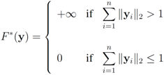
and . Finally the value for is given by . When one has . For clarity sake we collect the above results in Table 1.

Table 1. norm–ball radius correspondence for three different norms and fixed .

F(x)	r(z)
	||z − Bw||1
	||z − Bw||2
	||z − Bw||∞

Table 1. norm–ball radius correspondence for three different norms and fixed .

F(x)	r(z)
	||z − Bw||1
	||z − Bw||2
	||z − Bw||∞

In the algorithm described below the norm is denoted just by (numerical experiments presented in Section 5 are conducted with all three norms). The monitoring algorithm we propose is the following.

Algorithm 4.1Threshold monitoring algorithm.

• 1. Set .
• 2. Until end of stream.
• 3.    Set , (i.e., remember “initial" values for the vectors).
• 4.    Set (for definition of w see Equation (12)).
• 5.    Set .
• 6.    If for each
        go to step 5
     else
        go to step 3

In what follows, we assume that transmission of a double precision real number amounts to broadcasting one message. The message computation is based on the assumption that all nodes are updated by a new text simultaneously. When mean update is required, a coordinator (root) requests and receives messages from the nodes.

We next count a number of messages that should be broadcast per one iteration if the local constraint δ is violated at least at one node. We shall denote the set of all nodes by N, the set of nodes complying with the constraint by , and the set of nodes violating the constraint by (so that ). The cardinality of the sets is denoted by respectively, so that . Assuming one has the following:

• 1. nodes violators transmit their scalar ID and new coordinates to the root ( messages).
• 2. the root sends scalar requests for new coordinates to the complying nodes ( messages).
• 3. the complying nodes transmit new coordinates to the root ( messages).
• 4. root updates itself, computes new distance δ to the surface, and sends δ to each node ( messages).

This leads to total of

(14)

We conclude the section with three remarks. The first one compares conservatism of Algorithm 4.1 and the one suggested in [8]. The second one again compares the ball cover suggested in [8] and application of Algorithm 4.1 with l₁ norm. The last one shows by an example that Equation (8) fails when is substituted by . Significance of this negative result becomes clear in Section 5.

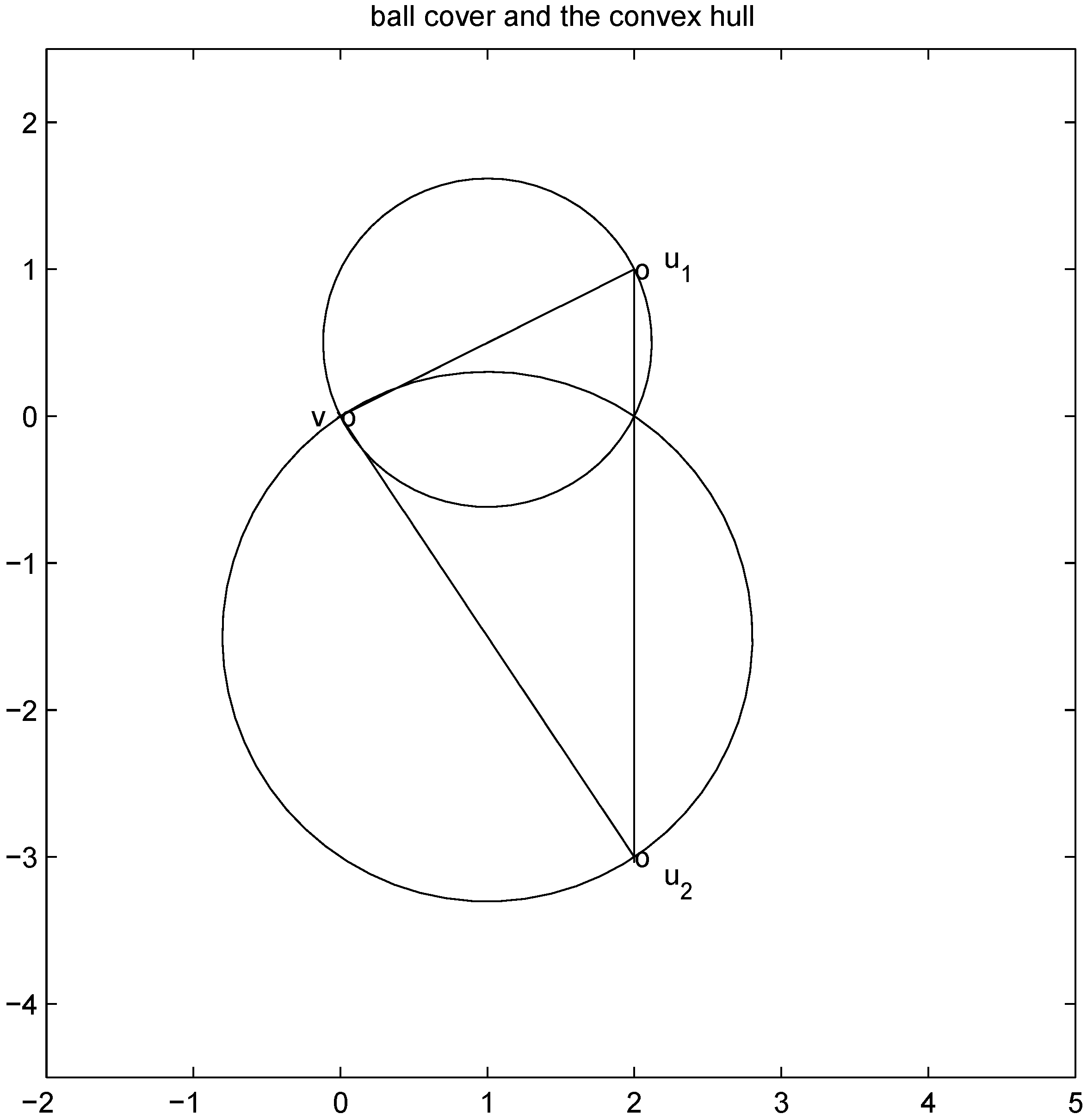
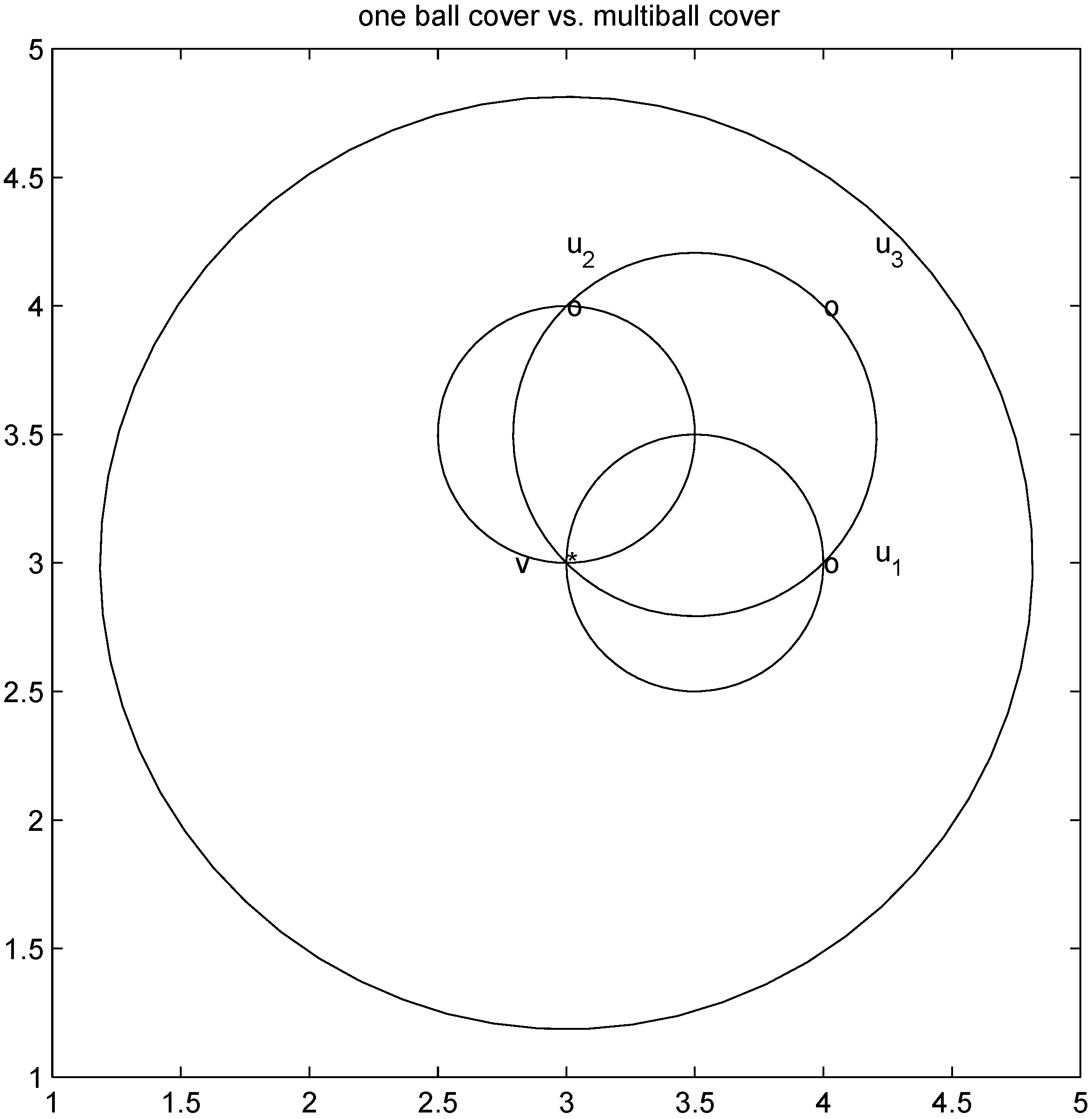
Remark 4.1 Let ,and . If the Step 6 inequality holds for each node, then each point of the ball centered at with radius is contained in the l₂ ball of radius δ centered at v (see Figure 2). Hence the sufficient condition offered by Algorithm 4.1 is more conservative than the one suggested in [8].

Figure 2. conservative cover by a single l₂ ball.

Figure 2. conservative cover by a single l₂ ball.

Algorithm 4.1 can be executed with a variety of different norms, and, as we show next, l₂ might not be the best one when communication between the nodes should be minimized.

Remark 4.2 Let ,

thedistance is given by the l₁ norm, and the aim is to monitor the inequality . Let

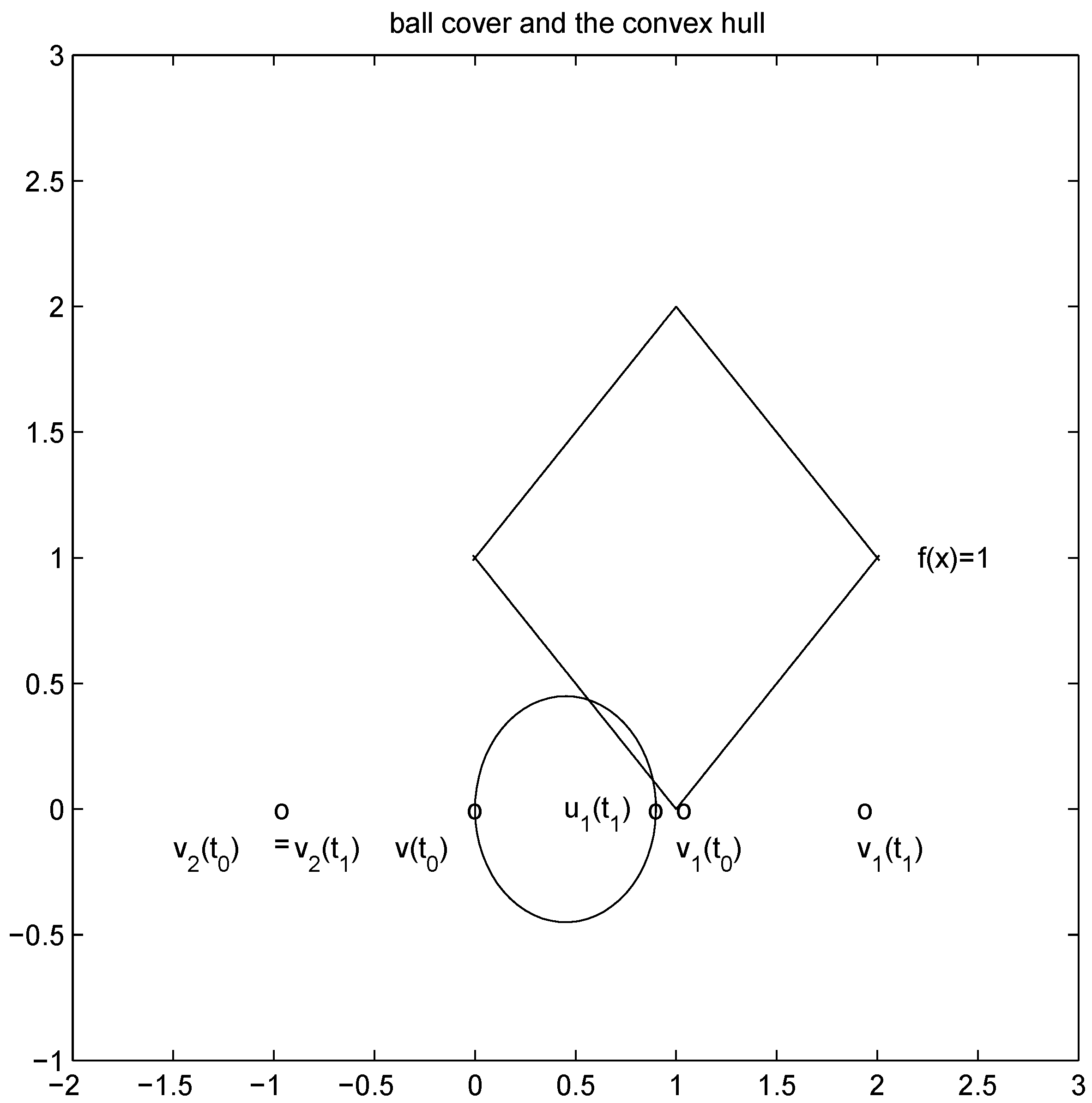
We first consider the “ball cover" construction suggested in [8]. With this data with , and with . At the same time . It is easy to see that the l₂ ball of radius centered at intersects the l₁ ball of radius 1 centered at (see Figure 3). Hence the algorithm suggested in [8] requires nodes to communicate at time t₁.

On the other hand the l₁ distance from to the set is 1, and since

Algorithm 4.1 requires no communication between nodes at time t₁. In this particular case the sufficient condition offered by Algorithm 4.1 is less conservative than the one suggested in [8].

Figure 3. l₂ ball cover requires communication.

Figure 3. l₂ ball cover requires communication.

Remark 4.3It is easy to see that inclusion Equation (8) fails when is an l₁ ball of radius centered at . Indeed, when, for example,

(see Figure 4) one has

In the next section we apply Algorithm 4.1 to a real life data and report number of required mean computations.

Figure 4. failed cover by l₁ balls.

Figure 4. failed cover by l₁ balls.

5. Experimental Results

We apply Algorithm 4.1 to data streams generated from the Reuters Corpus RCV1–V2. The data is available from [16] and consists of 781,265 tokenized documents with DID (document ID) ranging from 2651 to 810596.

The methodology described below attempts to follow that presented in [8]. We simulate n streams by arranging the feature vectors in ascending order with respect to DID, and selecting feature vectors for the stream in the round robin fashion.

In the Reuters Corpus RCV1–V2 each document is labeled as belonging to one or more categories. We label a vector as “relevant" if it belongs to the “CORPORATE/INDUSTRIAL" (“CCAT") category, and “spam" otherwise. Following [9] we focus on three features: “bosnia", “ipo", and “febru". Each experiment was performed with 10 nodes, where each node holds a sliding window containing the last 6700 documents it received.

First we use 67,000 documents to generate initial sliding windows. The remaining 714,265 documents are used to generate data streams, hence the selected feature information gain is computed 714,265 times. Based on all the documents contained in the sliding window at each one of the 714,266 time instances, we compute and graph 714,266 information gain values for the feature “bosnia" (see Figure 5).

For the experiments described below the threshold value r is predefined, and the goal is to monitor the inequality while minimizing communication between the nodes. From now on we shall assume simultaneous arrival of a new text at each node.

Figure 5. information gain values for the feature “bosnia”.

Figure 5. information gain values for the feature “bosnia”.

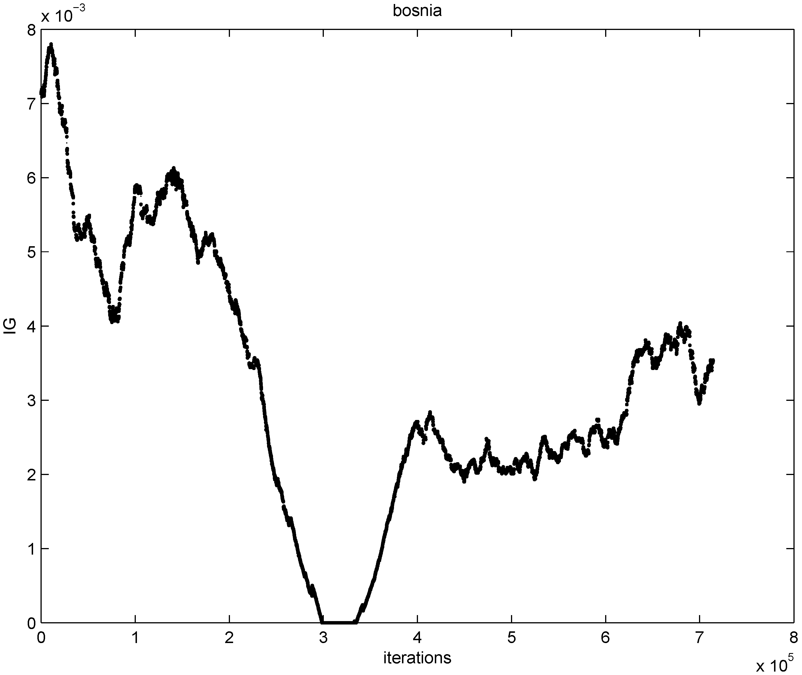
As new texts arrive, the local constraint (i.e., inequalities ) at each node is verified. If at least one node violates the local constraint, the average is updated. Our numerical experiment with the feature “bosnia", the l₂ norm, and the threshold (reported in [8] as the threshold for feature “bosnia" incurring the highest communication cost) shows overall 4006 computation of the mean vector. An application of Equation (14) yields 240,360 messages. We repeat this experiment with l_∞, and l₁ norms. The results obtained and collected in Table 2 show that the smallest number of the mean updates is required for the l₁ norm.

Table 2. number of mean computations, messages, and crossings per norm for feature “bosnia" with threshold .

Distance	Mean Comps	Messages	LL	LG	GL	GG
l2	4006	240,360	959	2	2	3043
l∞	3801	228,060	913	2	2	2884
l1	3053	183,180	805	2	2	2244

Table 2. number of mean computations, messages, and crossings per norm for feature “bosnia" with threshold .

Distance	Mean Comps	Messages	LL	LG	GL	GG
l2	4006	240,360	959	2	2	3043
l∞	3801	228,060	913	2	2	2884
l1	3053	183,180	805	2	2	2244

Throughout the iterations the mean goes through a sequence of updates, and the values may be larger than, equal to, or less than the threshold r. We monitor the case the same way as that of . In addition to the number of mean computations, we collect statistics concerning “crossings" (or lack of thereof), i.e., number of instances when the location of the mean v and its update relative to the surface are either identical or different. Specifically over the monitoring period we denote by:

• 1. “LL" the number of instances when and ,
• 2. “LG" the number of instances when and ,
• 3. “GL" the number of instances when and ,
• 4. “GG" the number of instances when and .

The number of “crossings" is reported in the last four columns of Table 2.

Note that variation of vectors does not have to be uniform. Taking on account distribution of signals at each node may lead to additional communication savings. We illustrate this statement by a simple example involving just two nodes. If, for example, there is a reason to believe that

(15)

then the number of node violations may be reduced by imposing node dependent constraints

so that the faster varying signal at the second node enjoys larger “freedom" of change, while the inequality

holds true. Assignments of “weighted" local constraints requires information provided by Equation (15). With no additional assumptions about signal distribution, this information is not available. Unlike [11] we refrain from making assumptions regarding possible underlying data distributions, instead we estimate the weights as follows:

• 1. Start with the initial set of weights
  (16)
• 2. As texts arrive at the next time instance each node computes
  If at time a local constraint is violated, then, in addition to messages (see Equation (14)), each node j broadcasts to the root, the root computes , and transmits the updated weights
  back to node j.

Broadcasts of weights cause increase of total number of messages per iteration to

(17)

With inequalities in Step 6 of Algorithm 4.1 substituted by the number of mean computations is reported in Table 3.

It is of interest to compare results presented in Table 3 with those reported, for example, in [9]. The comparison, however, is not an easy task. While [9] reports the threshold as the threshold value that incurred the highest communication cost, the paper leaves the concept of “communication cost" undefined (we define transmission of a double precision real number as a single “message"). In addition [9] provides a graph of “Messages vs. Threshold" only. It appears that the maximal value of “bosnia Messages vs. Threshold" graph is somewhere between 100,000 and 200,000.

Table 3. number of mean computations, messages, and crossings per norm for feature “bosnia" with threshold , and stream dependent local constraint .

Distance	Mean Comps	Messages	LL	LG	GL	GG
l2	2388	191,040	726	2	2	1658
l∞	2217	177,360	658	2	2	1555
l1	1846	147,680	611	2	2	1231

Table 3. number of mean computations, messages, and crossings per norm for feature “bosnia" with threshold , and stream dependent local constraint .

Distance	Mean Comps	Messages	LL	LG	GL	GG
l2	2388	191,040	726	2	2	1658
l∞	2217	177,360	658	2	2	1555
l1	1846	147,680	611	2	2	1231

We repeat the experiments with “ipo" and “febru" and report the results in Table 4 and Table 5 respectively. The results obtained with stream dependent local constraints is a significant improvement over those presented in [10]. Consistent with the results in [10] l₁ norm comes up as the norm that requires smallest number of mean updates in all reported experiments.

Table 4. number of mean computations, messages, and crossings per norm for feature “febru" with threshold , and stream dependent local constraint .

Distance	Mean Comps	Messages
l2	1491	119,280
l∞	1388	111,040
l1	1304	104,320

Table 4. number of mean computations, messages, and crossings per norm for feature “febru" with threshold , and stream dependent local constraint .

Distance	Mean Comps	Messages
l2	1491	119,280
l∞	1388	111,040
l1	1304	104,320

Table 5. number of mean computations, messages, and crossings per norm for feature “ipo" with threshold , and stream dependent local constraint .

Distance	Mean Comps	Messages
l2	7656	612,480
l∞	7377	590,160
l1	6309	504,720

Table 5. number of mean computations, messages, and crossings per norm for feature “ipo" with threshold , and stream dependent local constraint .

Distance	Mean Comps	Messages
l2	7656	612,480
l∞	7377	590,160
l1	6309	504,720

6. Future Research Directions

In what follows we briefly outline a number of immediate research directions we plan to pursue.

The local constraints introduced in this paper depend on history of a data stream at each node, and variations over time contribute uniformly to local constraints. Attaching more weight to recent changes than to older ones may contribute to further improvement of monitoring process.

Table 6 (borrowed from [10]) shows that in about 75% of instances (3034 out of 4006) the mean is updated because of a single node violation. This observation naturally leads to the idea of clustering nodes, and independent monitoring of the node clusters equipped with a coordinator. The monitoring will become a two step procedure. At the first step node violations are checked in each node separately. If a node violates its local constraint, the corresponding cluster computes updated cluster coordinator. At the second step, violations of local constraints by coordinators are checked, and if at least one violation is detected the root is updated. Table 6 indicates that in most of the instances only one coordinator will be effected, and, since communication within cluster requires less messages, the two step procedure briefly described above has a potential to bring additional savings.

Table 6. number of nodes simultaneously violating local constraints. for feature “bosnia" with threshold , and l₂ norm

nodes	violations
1	3034
2	620
3	162
4	70
5	38
6	26
7	34
8	17
9	5
10	0

Table 6. number of nodes simultaneously violating local constraints. for feature “bosnia" with threshold , and l₂ norm

nodes	violations
1	3034
2	620
3	162
4	70
5	38
6	26
7	34
8	17
9	5
10	0

We note that a standard clustering problem is often described as “…finding and describing cohesive or homogeneous chunks in data, the clusters" (see e.g., [17]). The monitoring data streams problem requires to assign to the same cluster i nodes so that the total change within cluster is minimized, i.e., nodes with different variations that cancel out each other as much as possible should be assigned to the same cluster. Hence, unlike classical clustering procedures, one needs to combine “dissimilar" nodes together. This is a challenging new type of a difficult clustering problem.

Realistically, verification of inequality should be conducted with an error margin (i.e., the inequality should be investigated, see [9]). A possible effect of an error margin on the required communication load is another direction of future research.

7. Conclusions

Monitoring streams over distributed systems is an important and challenging problem with a wide range of applications. In this paper we build on the approach for monitoring an arbitrary threshold functions suggested in [10], and introduce stream dependent local constraints that serve as a feedback monitoring mechanism. The obtained preliminary results indicate substantial improvement over those reported in [10], and demonstrate that monitoring with l₁ norm requires fewer updates than that with l_∞ or l₂ norm.

References

- Madden, S.; Franklin, M.J. An Architecture for Queries Over Streaming Sensor Data. In Proceedings of the ICDE 02, San Jose, CA, 26 February–1 March 2002; pp. 555–556.
- Dilman, M.; Raz, D. Efficient Reactive Monitoring. In Proceedings of the Twentieth Annual Joint Conference of the IEEE Computer and Communication Societies, Anchorage, Alaska, 2001; pp. 1012–1019.
- Zhu, Y.; Shasha, D. Statestream: Statistical Monitoring of Thousands of Data Streamsin Real Time. In Proceeding of the 28th international conference on Very Large Data Bases (VLDB), Hong Kong, China, 2002; pp. 358–369.
- Yi, B.-K.; Sidiropoulos, N.; Johnson, T.; Jagadish, H.V.; Faloutsos, C.; Biliris, A. Online Datamining for Co–Evolving Time Sequences. In Proceedings of ICDE 00IEEE Computer Society, San Diego, CA, 2000; pp. 13–22.
- Manjhi, A.; Shkapenyuk, V.; Dhamdhere, K.; Olston, C. Finding (Recently) Frequent Items in Distributed Data Streams. In Proceedings of the 21st International Conference on Data Engineering (ICDE 05), Tokyo, Japan, 2005; pp. 767–778.
- Wolff, R.; Bhaduri, K.; Kargupta, H. Local L2-Thresholding Based Data Mining in Peer-to-Peer Systems. In Proceedings of the SIAM International Conference on Data Mining (SDM 06), Bethesda, MD, USA, 2006; pp. 430–441.
- Wolff, R.; Bhaduri, K.; Kargupta, H. A generic local algorithm with applications for data mining in large distributed systems. IEEE Trans. Knowl. Data Eng. 2009, 21, 465–478. [Google Scholar] [CrossRef]
- Sharfman, I.; Schuster, A.; Keren, D. A geometric approach to monitoring threshold functions over distributed data streams. ACM Trans. Database Syst. 2007, 23, 23–29. [Google Scholar]
- Sharfman, I.; Schuster, A.; Keren, D. A Geometric Approach to Monitoring Threshold Functions over Distributed Data Streams. In Ubiquitous Knowledge Discovery; May, M., Saitta, L., Eds.; Springer–Verlag: New York, NY, USA, 2010; pp. 163–186. [Google Scholar]
- Kogan, J. Feature Selection over Distributed Data Streams through Convex Optimization. In Proceedings of the Twelfth SIAM International Conference on Data Mining (SDM 2012), Anaheim, CA, USA, 2012; pp. 475–484.
- Keren, D.; Sharfman, I.; Schuster, A.; Livne, A. Shape sensitive geometric monitoring. IEEE Trans. Knowl. Data Eng. 2012, 24, 1520–1535. [Google Scholar] [CrossRef]
- Gray, R.M. Entropy and Information Theory; Springer–Verlag: New York, NY, USA, 1990; pp. 119–162. [Google Scholar]
- Hinrichsen, D.; Pritchard, A.J. Real and Complex Stability Radii: A Survey. In Controlof Uncertain Systems; Hinrichsen, D., Pritchard, A.J., Eds.; Birkhauser: Boston, MA, USA, 1990; pp. 119–162. [Google Scholar]
- Rudin, W. Principles of Mathematical Analysis; McGraw-Hill: New York, NY, USA, 1976. [Google Scholar]
- Rockafellar, R.T. Convex Analysis; Princeton University Press: Princeton, NJ, USA, 1970. [Google Scholar]
- Bottou, L. Home Page. Available online: leon.bottou.org/projects/sgd (accessed on 14 September 2012).
- Mirkin, B. Clustering for Data Mining: A Data Recovery Approach; Chapman & Hall/CRC: Boca Raton, FL, USA, 2005. [Google Scholar]
© 2012 by the authors; licensee MDPI, Basel, Switzerland. This article is an open-access article distributed under the terms and conditions of the Creative Commons Attribution license (http://creativecommons.org/licenses/by/3.0/).
Share and Cite
Malinovsky, Y.; Kogan, J. Monitoring Threshold Functions over Distributed Data Streams with Node Dependent Constraints. Algorithms 2012, 5, 379-397. https://doi.org/10.3390/a5030379
Malinovsky Y, Kogan J. Monitoring Threshold Functions over Distributed Data Streams with Node Dependent Constraints. Algorithms. 2012; 5(3):379-397. https://doi.org/10.3390/a5030379
Chicago/Turabian StyleMalinovsky, Yaakov, and Jacob Kogan. 2012. "Monitoring Threshold Functions over Distributed Data Streams with Node Dependent Constraints" Algorithms 5, no. 3: 379-397. https://doi.org/10.3390/a5030379
APA StyleMalinovsky, Y., & Kogan, J. (2012). Monitoring Threshold Functions over Distributed Data Streams with Node Dependent Constraints. Algorithms, 5(3), 379-397. https://doi.org/10.3390/a5030379