1. Introduction
Volcanism combines complex geophysical and geochemical processes that vary in composition, duration, and intensity from location to location and episode to episode. Therefore, successful eruption forecasting will only be achieved through the use of methods that simultaneously weigh empirical experience and real time interpretation of processes [
1]. Event trees have proven to be useful tools for forecasting volcanic activity [
2,
3,
4]. In 2002, Newhall and Hoblitt outlined a generic event tree structure for forecasting various types of volcanic activity and associated hazards. This process has since been adopted and improved upon by a variety of researchers to forecast volcanic activity at various locations throughout the world [
5,
6,
7,
8,
9,
10,
11,
12]. These event tree implementations require probability density functions to be manually derived on a volcano-by-volcano basis. This means every volcano being monitored will have a unique and unvalidated set of statistical functions driving its prediction process. As a result, each instance of the algorithm will use subjectively selected detection thresholds that possess a unique and unquantified false alarm rate.
This research initiative aims to improve and standardize the event tree forecasting process. The method employed here also uses Newhall and Hoblitt’s generic event tree infrastructure. However, we have augmented its decision making process with a suite of empirical statistical models that are derived through logistic regression. Each model is constructed from a geographically diverse dataset that was assembled from a collection of historic volcanic unrest episodes. The dataset consists of monitoring measurements (e.g., seismic), source modeling results, and historic eruption activity information. The regression uses a generalized linear model routine (GLMR) that assumes a binominal response variable and employs a logit linking function. This process allows for trends in the relationship between modeling results, monitoring data, historic information, and the known outcome of the events to drive the formulation of the statistical models. It yields a static set of logistic models that weight the contributions of empirical experience and monitoring data relative to one another. They estimate the probability of a particular event occurring based on the current values of a set of predefined explanatory variables, are highly transportable, and do not need to be redefined for each volcano being monitored. This provides a simple mechanism for simultaneously accounting for the geophysical changes occurring within the volcano and the historic behavior of analog volcanoes in short-term forecasts. In addition, a rigorous cross validation process is used to document the algorithm’s performance, identify optimum detection thresholds, and quantify false alarm rates. The methodology is easily extensible, where recalibration can be performed or new branches added to the decision making process with relative ease. Such a system could aid federal, state, and local emergency management officials in determining the proper response to an impending eruption and can be easily deployed by a National Volcano Early Warning System (NVEWS).
This paper is organized into several sections. It begins with an overview of the volcanic eruption forecasting algorithm, logistic models, and cross validation analysis. The next section provides a detailed discussion of forecasts generated by the algorithm. The final section discusses the conclusions that can be drawn from this work and provides an overview of future research initiatives that may improve the algorithm’s performance.
2. Eruption Forecasting Algorithm
An event tree is a decision making framework that estimates the probability of a set of pre-defined events using a tree like decision making process. Each branch or node of the tree represents a set of possible outcomes for a particular event, which increase in specificity with each step. Progression to the next branch is accomplished when the probability estimate for the preceding node exceeds a pre-defined threshold. Our algorithm is rooted in a general state of unrest and grows to forecast volcanic activity in increasing detail, such as the probability of eruption, intensity, and location.
Figure 1.
Schematic representation of the event tree, where the clone label indicates the tree structure at that point is identical to that below. The color code represents the USGS ground-based hazard declarations and are superimposed over their respective event tree branch.
Figure 1.
Schematic representation of the event tree, where the clone label indicates the tree structure at that point is identical to that below. The color code represents the USGS ground-based hazard declarations and are superimposed over their respective event tree branch.
The event tree utilized in this research is shown in
Figure 1. Each node estimates the conditional probability for a specific event via Bayes theorem, which is defined as
where P(n − 1|n) is the likelihood, P(n) is the prior probability, P(n − 1) is the marginal probability, P(n|n − 1) is the posterior probability, the prime symbol represents the complement, and n is the event tree node. Our event tree implementation is comprised of the following nodes:
• Node 1. Unrest: Does the geophysical activity at the selected volcano exceed a predetermined threshold? Geophysical activity includes heightened seismicity or surface deformation. If the amount of unrest exceeds a predefined threshold, the decision making process progresses to the next branch, otherwise it terminates and restarts when new data are available. If the predefined threshold is exceeded, the probability that unrest is occurring equals one, which is given by
where
ν1 is the summation of several explanatory variables that are defined in
Section 2.3.
• Node 2. Magmatic Intrusion: Is the observed unrest the result of a magmatic intrusion? Fluid motion can be detected from the presence of heightened levels of seismicity having specific spectral characteristics or continuous or rapidly varying surface deformation. Possible causes of unrest that are not related to fluid motion or not indicative of an impending eruption include tectonic and geothermal activity. If the unrest is related to fluid motion, the process progresses to the next branch, otherwise it terminates and restarts when new data are available. The probability that an intrusive event is occurring is given by
where P(2) is defined as
and
X2,N is a node specific set of
N independent explanatory variables described in
Section 2.4.
• Node 3. Eruption: Does the detected fluid motion have the potential to reach the surface and cause an eruption? If the source of the unrest is a magmatic intrusion with associated seismicity, the probability that the fluid will reach the surface may be high if that particular volcano has a historically high eruption frequency. If the observed, modeled, and historic information support this hypothesis, the algorithm moves to the next branch, otherwise it terminates and restarts when new data are available. The probability that an eruption will occur is given by
where P(3) is defined as
and
X3,N is a node specific set of
N independent explanatory variables described in
Section 2.4.
• Node 4.
Intensity: Will the eruption intensity exceed a VEI of 1? The determination of the intensity will be driven by the training dataset defined in
Table 1. The probability of the eruption’s intensity exceeding a Volcanic Explosivity Index, (
V EI), of 1 is given by
where P(4) is defined as
and
X4,N is a node specific set of
N independent explanatory variables described in
Section 2.4.
• Node 5. Vent Location: Where is the eruption likely to occur? A vent location probability map is generated and the area with the highest probability of occurrence is identified as the likely eruption location. Given that the previous conditions are satisfied, the most probable vent location may be those with collocated surface deformation and seismicity. The probability of an eruption occurring at any location in a specified area is given by
where
J is the total number of probable vent locations,
j is the location under consideration, and
P(5) is defined in
Section 2.5.
The probability of an event occurring at a particular event tree node is defined as
where
l is the event tree node for which the probability is being calculated. For example, the probability of an eruption occurring at the
jth location is calculated from the product,
P(Θ
1)
P(Θ
2)
P(Θ
3)
P(Θ
4)
![]()
, whereas the probability of an eruption occurring at a given volcano is estimated by
P(Θ
1)
P(Θ
2)
P(Θ
3).
Table 1.
Raw logistic regression training data.
Table 1.
Raw logistic regression training data.
| Episode | Response Var. | Independent Variable |
|---|
| Year | Volcano | VEI | Er | In | MM | TNE | TCSM | Days | TEH | Ref. |
| 1993 | Medicine Lake(2,3,4) | 0 | 0 | 0 | 0 | 115 | 6.0e + 21 | 2492 | 1 | [13] |
| 1993 | Makushin(3,4) | 0 | 0 | 1 | 1 | 0 | 0 | 365 | 12 | [14] |
| 1994 | Hengill(2,3,4) | 0 | 0 | 1 | 1 | 63450 | 7.7e + 23 | 1607 | 0 | [15] |
| 1995 | Trident(2,3,4) | 0 | 0 | 1 | 1 | 69 | 3.2e + 19 | 137 | 13 | [16] |
| 1996 | Lassen Peak(2,3,4) | 0 | 0 | 0 | 0 | 110 | 3.4e + 21 | 1460 | 1 | [17] |
| 1996 | Eyjafjallajökull(2,3,4) | 0 | 0 | 1 | 1 | 144 | 5.2e + 19 | 114 | 2 | [18] |
| 1996 | Akutan(2) | 0 | 0 | 1 | 1 | 1194 | 7.6e + 22 | 32 | 34 | [19] |
| 1996 | Iliamna(2,3,4) | 0 | 0 | 1 | 1 | 1477 | 2.1e + 21 | 382 | 2 | [20] |
| 1996 | Peulik(2,3,4) | 0 | 0 | 1 | 1 | 0 | 0 | 365 | 2 | [21,22] |
| 1997 | Kilauea(2,3) | 1 | 1 | 1 | 0 | 1869 | 1.9e + 22 | 20 | 63 | [23] |
| 1998 | Kiska(2,3,4) | 0 | 0 | 0 | 0 | 0 | 0 | 365 | 3 | [24] |
| 1998 | Grimsv"{o]tn(2,3,4) | 3 | 1 | 1 | 1 | 31 | 9.4e + 20 | 10 | 29 | [25] |
| 1999 | Shishaldin(2,3,4) | 3 | 1 | 1 | 0 | 688 | 9.0e + 22 | 42 | 34 | [26] |
| 1999 | Fisher(2,3,4) | 0 | 0 | 0 | 1 | 0 | 0 | 365 | 1 | [27] |
| 2000 | Katla(2,3,4) | 0 | 0 | 1 | 1 | 12460 | 1.2e + 23 | 2190 | 4 | [28] |
| 2000 | Kilauea(2,3,4) | 0 | 0 | 0 | 0 | 48 | 5.8e + 20 | 13 | 63 | [29] |
| 2000 | Three Sisters(2,3,4) | 0 | 0 | 1 | 1 | 0 | 0 | 1460 | 1 | [22] |
| 2000 | Hekla(2,3,4) | 3 | 1 | 1 | 1 | 196 | 3.4e + 20 | 15 | 9 | [30,31] |
| 2000 | Eyjafjallajökull(2,3,4) | 0 | 0 | 1 | 1 | 170 | 4.1e + 20 | 365 | 2 | [32] |
| 2001 | Etna(2,3,4) | 2 | 1 | 1 | 1 | 414 | 1.0e + 23 | 28 | 115 | [33] |
| 2001 | Okmok(4) | 0 | 0 | 0 | 1 | 19 | 8.1e + 21 | 2 | 16 | [34] |
| 2001 | Aniakchak(2,3,4) | 0 | 0 | 0 | 1 | 13 | 5.8e + 20 | 64 | 1 | [35] |
| 2002 | Hood(2,3,4) | 0 | 0 | 0 | 0 | 86 | 7.8e + 22 | 60 | 2 | [36] |
| 2002 | Etna(2,3,4) | 3 | 1 | 1 | 1 | 353 | 2.1e + 23 | 94 | 115 | [37] |
| 2003 | Veniaminof(2) | 2 | 1 | 1 | 1 | 103 | 6.2e + 20 | 1050 | 22 | [38] |
| 2004 | Grimsvötn(2,3,4) | 3 | 1 | 0 | 0 | 920 | 6.3e + 21.9 | 490 | 29 | [39] |
| 2004 | Spurr(3,4) | 0 | 0 | 0 | 0 | 2743 | 5.1e + 20 | 239 | 2 | [40,41] |
| 2004 | Etna(2,3,4) | 1 | 1 | 1 | 1 | 156 | 4.8e + 21 | 186 | 115 | [42] |
| 2004 | Saint Helens(2,3,4) | 2 | 1 | 1 | 1 | 1094 | 1.5e + 23 | 21 | 14 | [43] |
| 2005 | Augustine(2,3,4) | 3 | 1 | 1 | 1 | 2007 | 3.1e + 20 | 80 | 9 | [44] |
| 2006 | Korovin(2,3,4) | 1 | 1 | 0 | 1 | 377 | 1.4e + 21 | 329 | 7 | [45,46] |
| 2007 | Pavlof(2) | 2 | 1 | 1 | 0 | 2 | 8.8e + 18 | 30 | 39 | [47] |
| 2007 | Upptyppingar(2,3,4) | 0 | 0 | 1 | 0 | 3124 | 6.5e + 20 | 133 | 0 | [48] |
| 2008 | Yellowstone(2,3) | 0 | 0 | 1 | 1 | 2594 | 6.9e + 22 | 49 | 0 | [49] |
| 2008 | Paricutin(2,3,4) | 0 | 0 | 0 | 0 | 0 | 0 | 21900 | 1 | [50] |
| 2008 | Hengill | 0 | 0 | 0 | 0 | 3309 | 1.1e + 24 | 10 | 0 | [51] |
| 2008 | Okmok(2,3,4) | 4 | 1 | 1 | 1 | 464 | 4.9e + 21 | 100 | 16 | [34,52] |
| 2008 | Kasatochi(2,3,4) | 4 | 1 | 1 | 0 | 1489 | 7.4e + 24 | 22 | 1 | [53] |
| 2009 | Redoubt(2,3,4) | 3 | 1 | 1 | 1 | 4219 | 3.9e + 21 | 365 | 6 | [31] |
| 2010 | Eyjafjallajökull(2,3,4) | 4 | 1 | 1 | 1 | 4019 | 1.1e + 22 | 100 | 2 | [54] |
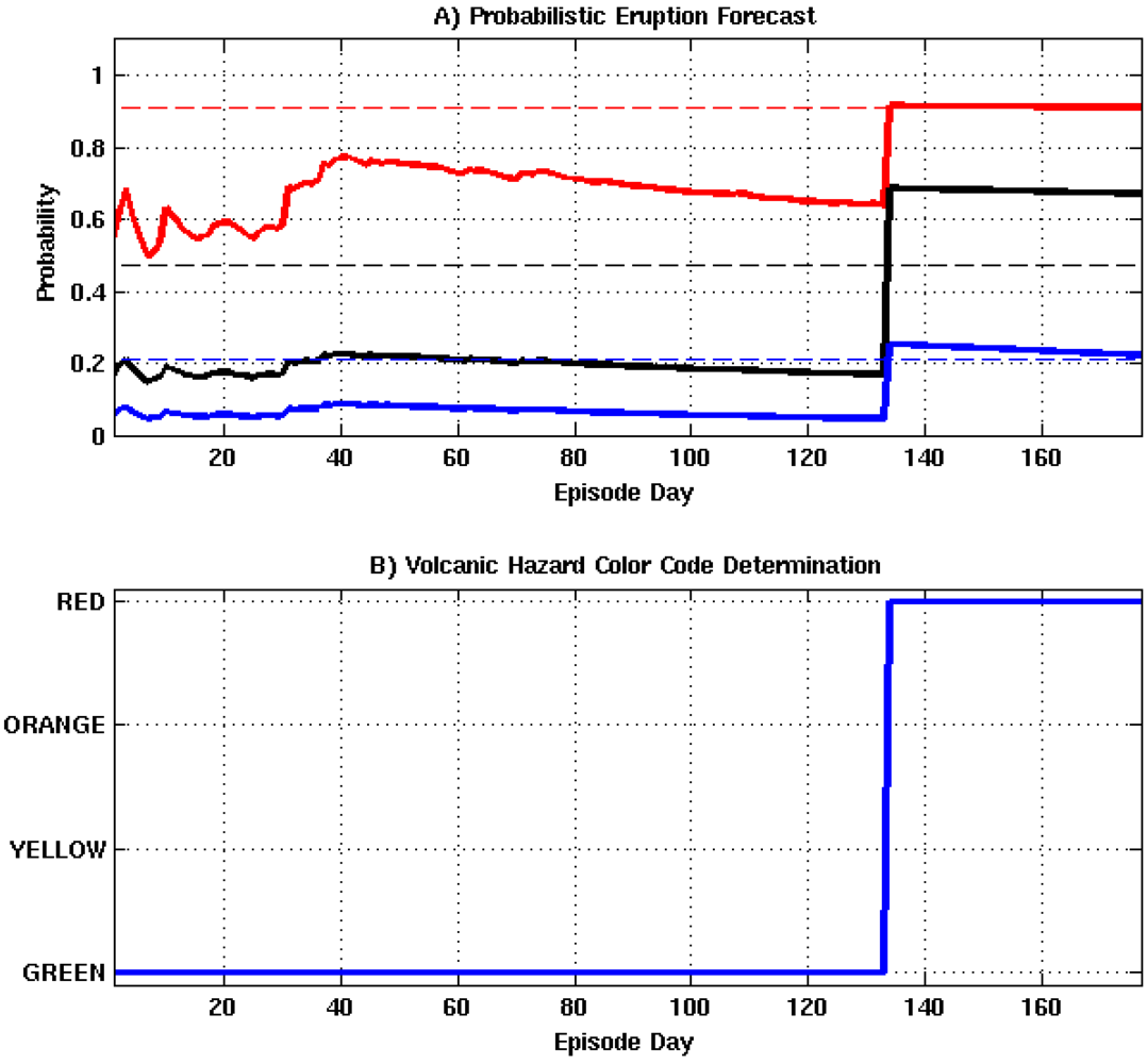
The event tree was adapted to issue warnings according to the United States Geological Survey (USGS) ground-based volcanic hazard system. Our system assigns colors ranging from green to red to a particular volcano according to its current eruption hazard condition, where green = normal, yellow = advisory, orange = watch, and red = warning.
Figure 1 shows the color code assignments relative to each stage of the event tree. The final color designation is set according to the point in the algorithm where processing is terminated. For example, if the algorithm is activated by a new unrest episode and is not allowed to progress past the eruption node, because the probability of occurrence does not exceed a predefined decision threshold, then the final hazard level is set to orange. However, if the algorithm were to progress to the intensity node the hazard level is set to red.
2.1. Logistic Regression
Logistic regression is a statistical modeling method used to analyze multivariate problems [
55,
56,
57]. It attempts to describe the complex relationship between a set of independent explanatory variables and a response variable. This popular modeling approach is used extensively in medical research, bioinformatics, and marketing analysis [
58]. It has also found use in geophysical applications, such as the prediction of landslides and rain rate [
59,
60].
The logistic function, f(z), is given by
where z is a value computed from a logistic model. The range of f(z) is bound between 0 and 1 over ±∞. Unlike other modeling techniques, a probability between 0 and 1 is guaranteed with logistic regression regardless of the value of z. The logistic model is the weighted summation of a set of explanatory variables, which is defined as
where β0 is a constant (intercept), βm are the weighting (regression) coefficients, and Xm are the explanatory variables. Values of β0 and βm are determined through maximum likelihood estimation via a GLMR. This requires a training dataset consisting of a collection of observations that relate the outcome of a particular event to the explanatory variables.
Using this technique, we derived a suite of logistic models to compute the prior probability for the nth event tree node. These models are defined as the conditional probability
where
θn is the outcome (
i.e., 1 or 0) of the event represented by the
nth node and
zn is its respective logistic model. Weighting coefficients for each logistic model are described in
Section 2.4.
The goodness-of-fit (G) of a logistic model is often assessed using a likelihood ratio test [
56]. The test statistic is derived from the difference between the deviance,
−2ln(Ln), of the null and full models, where the null model is simply a constant with no associated explanatory variables. The deviance is similar to the residual sums of squares metric from ordinary least squares regression in the sense that it attempts to estimate the discrepancy between the modeled and observed data. Thus, the quality of the regression model decreases with increasing deviance. Here
G is estimated via the ratio
where Lnull and Lfull are the likelihoods of the null and full models. The test statistic is x2 distributed, where its degrees of freedom, df, are equivalent to the number of constrained predictors (explanatory variables) in the logistic model. Statistical significance of the difference is estimated using a hypothesis test which compares the p-value of the test statistic to a predefined significance level (0.05), where the null hypothesis states the null model fits the data better than the full model. If there is strong evidence against the null hypothesis (e.g., p < 0.05), then it can be rejected in favor of the full model.
2.2. Training Data
A database comprised of monitoring data, source modeling results, and historic eruption information from a series of volcanic unrest episodes is required for deriving the logistic model coefficients. Unfortunately, no such database existed in the public domain at the time of this study. Therefore, one had to be constructed for this research. Ideally, a large and diversified set of data is desired for identifying the set of explanatory variables that will produce the most robust logistic model. Moreover, it is also desirable to identify a large number of events that either culminate or fail to culminate into an eruption. However, published accounts of volcanic unrest events vary greatly in detail and do not contain a consistent set of observations. This problem is exasperated by the fact that events which eventually result in an eruption tend to be published, while those that fail are not. This has artificially biased the open literature toward eruptive events as opposed to those that eventually fail [
61]. As a result, only a small set of unrest events with known sources and a consistent set of explanatory variables could be identified for this research.
The database constructed for this work is listed in
Table 1. It is a collection of unrest events with a consistent set of observations whose causes were identified through source modeling. The 40 events in the database were gathered from various volcanoes in Northern America, Iceland, and Italy. For an event to be included in the database, a seismic catalog and modeling results that identify the source of the unrest must be available. These data were acquired from a combination of journal articles, technical reports, conference papers, and open seismic catalogs that are made freely available to the public by a number of organizations (e.g., USGS, ANSS, Icelandic Meteorological Institute) via the internet. It is assumed that this collection of events represent a random sample of volcanic activity in the northern hemisphere and is representative of this population.
Table 1 consists of eleven columns. The first two columns list the episode year and volcano of origin. Column three is the event’s (
V EI). The fourth column, (
Er), specifies whether the event culminated in an eruption, where true (eruption) and false (no eruption) outcomes are represented by a 1 or 0. The cause of the unrest is listed in column five, (
In), where a value of 1 or 0 states whether the source is a magmatic intrusion or not. Source modeling results are listed in column six, (
MM), where a value of 1 or 0 states if the source of the unrest can be modeled as a magmatic intrusion or not. The total number of earthquakes occurring over the course of the episode is listed in column seven, (
TNE). An estimate of the total cumulative seismic moment generated throughout the episode, (
TCSM), is listed in column eight. The duration of each episode in terms of days is listed in column nine, (
Days). The total number of eruptions at a particular site over the last 211 years is listed in column ten, (
TEH). This time span represents the extent of the Smithsonian Institute (
SI) global volcanism database of eruptions that are known to have occurred in modern history (post 1800) [
62]. It is meant to prevent overestimation of the probability of eruption at sites that typically display high levels of geologic activity but rarely erupt. The Yellowstone caldera is a prime example of where such a term is necessary. If historic eruption activity is not accounted for at Yellowstone, forecasts would show that an eruption is imminent (probability of eruption = 1.0) inside the caldera on an almost continuous basis. When historic eruptive activity is taken into consideration, the probability of eruption is adjusted to account for long periods of non-eruptive behavior. Finally the source of the information listed in each row is referenced in column eleven.
Superscripts above the volcano name represent that sample’s participation in the derivation of logistic coefficients for each node. Note that the logistic regression is performed after the TNE and T CSM columns are transformed to average values per day and the normalization factor (1e20dyn − cm) is applied to the cumulative seismic moment estimates.
2.3. Node 1: Detection of Volcanic Unrest
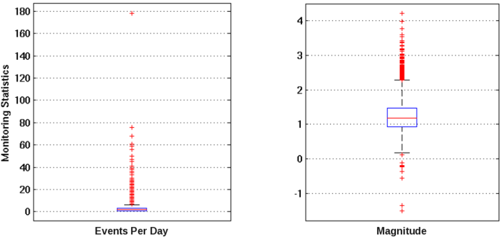
Anomalous geologic activity (e.g., volcanic unrest) is detected using the method described in [
63]. Historic information collected by a variety of multidisciplinary remote and in-situ sensing techniques is used to identify activity that is markedly different (
i.e., outliers) from past behavior. Discipline specific outlier thresholds are derived from
where c is a constant,
Q1 and
Q3 are the first and third quartiles of the sample distribution, and (
Q3−Q1) is the interquartile range [
64]. Unique thresholds are derived empirically on a volcano-by-volcano and monitoring discipline basis using Equation 15, where c is set empirically for each monitoring discipline.
The severity of the anomaly is estimated from the weighted summation of a collection of binary variables. The general form of the severity estimate is defined as
where βm are weighting coefficients and Xm are binary variables that are toggled from 0 to 1 when measurements from their respective monitoring discipline exceeds its outlier detection threshold. Here the functional form of Equation 16 is expressed as
where each binary variable is defined in
Table 2. In this case, all variables are weighted equally (
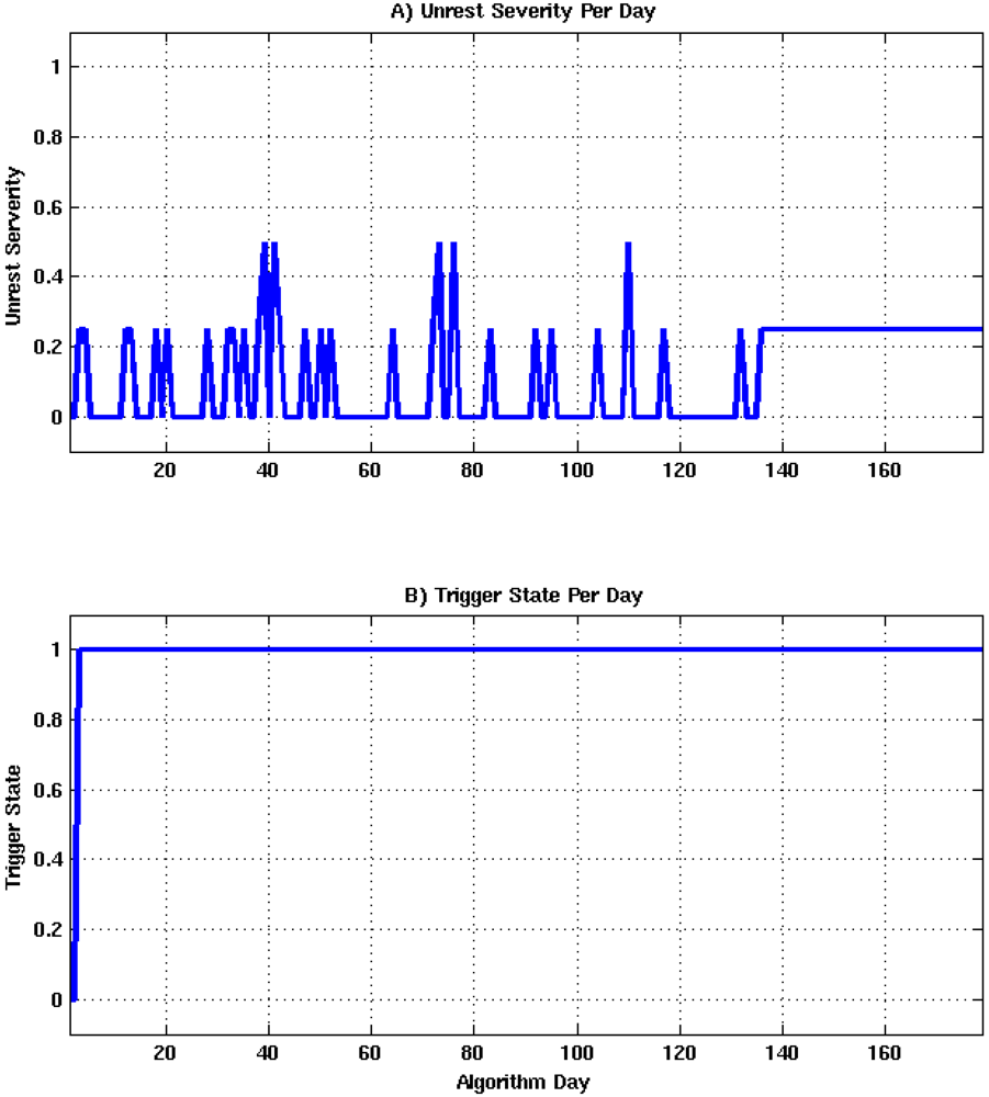
βm = 0.25) to allow activation of the forecasting algorithm upon the detection of unrest by one or more monitoring techniques. Severity declarations are based on the number of simultaneous cross-disciplinary detections, where
ν1 values of 0.25, 0.50, 0.75, and 1.0 represent low, moderate, heightened, and extreme levels of unrest. This triggering mechanism differs from those described in previously published event tree implementations (e.g., [
7]) through its use of outlier analysis for detection threshold estimation and the incorporation of source modeling information.
Table 2.
Explanatory variable names, descriptions, and possible values for node 1.
Table 2.
Explanatory variable names, descriptions, and possible values for node 1.
| Explanatory Variable | Description | Value |
|---|
| Xsr | Seismicity Rate | 0/1 |
| Xdf | Surface Deformation | 0/1 |
| Xlm | Large Magnitude | 0/1 |
| Xmd | Model Indicates Intrusion | 0/1 |
2.4. Nodes 2-4: Intrusion, Eruption, and Intensity
Ideally, the regression uses many combinations of random samples from the population we are attempting to model. After many iterations, a distribution of parameter estimates, such as the sample mean or regression coefficients, can be produced and their true value estimated. In this case, however, there are no additional data available. Therefore, a bootstrapping approach is used to estimate the distribution of logistic model coefficients for nodes 2, 3, and 4 using selected subsets of data from
Table 1.
Bootstrapping is a resampling technique that produces M datasets from a single set of random samples taken from a specific population. Each of the newly constructed datasets contains a random combination of samples that were drawn from the original dataset. Since a sample with replacement process is used, it is possible for each new dataset to contain multiple or no copies of any particular sample. Thus, the probability that a particular sample is selected for inclusion in a bootstrapped dataset each time a drawing is made is 1/N, where N is the number of samples in the original dataset.
Model coefficients for each node were estimated from the distributions generated after 50,000 bootstrapped GLMR iterations. The distributions for each of the logistic model coefficient appears to be bimodal. The two distributions represent cases where the regression is either properly or ill constrained. Situations where the regression is ill constrained caused the GLMR to fail after reaching its maximum number of iterations, which results in a bogus set of model coefficients. Conversely, properly constrained cases represent runs where the GLMR converges to a solution within its maximum number of iterations. Therefore, the ill constrained results are rejected as outliers and the properly constrained distributions are retained and used to estimate logistic model information. In all cases, the median value of the truncated distributions are used to estimate the coefficients for each model.
The logistic models for nodes 2, 3, and 4 are shown in Equations 18–20 and a description of each explanatory variable is listed in
Table 3. Node 3 (Equation 19) required an additional explanatory variable to account for the relationship between historic eruption activity and monitoring data. The likelihood ratio test for each model yielded p-values of 0.001, 0.014, and 0.007, which provides strong evidence against the null hypothesis for each node.
Table 3.
Logistic model explanatory variable names, descriptions, and possible range of values.
Table 3.
Logistic model explanatory variable names, descriptions, and possible range of values.
| Explanatory Variable | Description | Value |
|---|
| XMM | Unrest consistent with intrusion model | 0 or 1 |
| XNE | Average Number of Earthquakes Per Day | 0 – ∞ |
| XCSM | Average Normalized Cumulative Seismic Moment Per Day | 0 – ∞ |
| XDAYS | Episode Duration in Days | 0 – ∞ |
| XERH | Average Eruption History | 0 – ∞ |
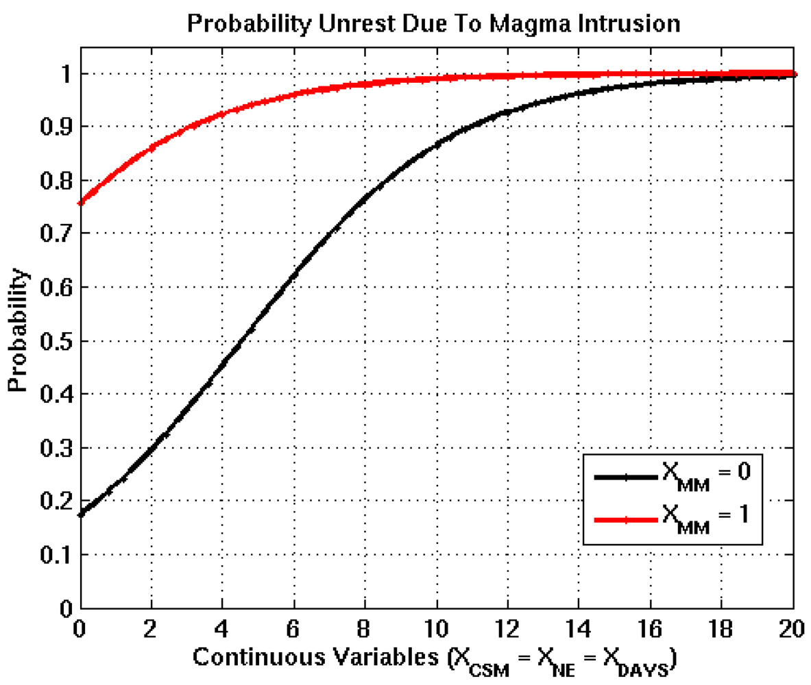
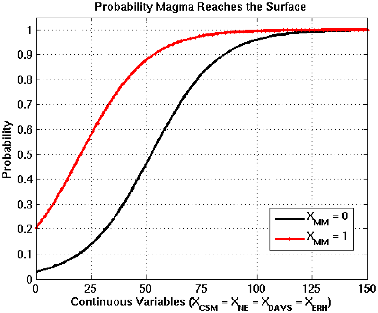
The influence of the source modeling results (XMM) on each logistic function is examined by setting all other explanatory variables equal to each other and plotting the model response for values ≥ 0.
Figure 2,
Figure 3,
Figure 4 show that positive modeling results increase the probability of occurrence for each node. In addition, each plot shows that even in the absence of positive modeling results, episodes producing large numbers of earthquakes and/or releasing large amounts of seismic energy have a high probability of being generated by a magmatic intrusion. Moreover, they also show that the probability of an eruption is non-zero when all explanatory variables are equal to zero. This result is reassuring, since eruptions have been known to occur without any precursory activity or warning.
Figure 2.
Logistic functions derived from bootstrapping process for the intrusion node, where the black and red curves represent XMM =0 and XMM =1. The transition of XMM from 0 to 1 increases the probability of occurrence by 0.60, which is the difference between the black and red curves when all continuous input variables are equal to 0.
Figure 3.
Logistic functions derived from bootstrapping process for the Eruption node, where the black and red curves represent XMM =0 and XMM =1. The transition of XMM from 0 to 1 increases the probability of occurrence by 0.17, which is the difference between the black and red curves when all continuous input variables are equal to 0.
Figure 4.
Logistic functions derived from bootstrapping process for the intensity node, where the black and red curves represent XMM =0 and XMM =1. The transition of XMM from 0 to 1 increases the probability of occurrence by 0.13, which is the difference between the black and red curves when all continuous input variables are equal to 0.
2.5. Node 5: Vent Location
The spatial probability density function (PDF) for estimating the probability of vent formation (V) at the jth location is derived from the data used for monitoring a particular volcanic center. Here the PDF is constructed from deformation data (Xdef) and the spatiotemporal distribution of seismic epicenters (Xseis). Combining this information yields the expression
where
J is the total number of probable vent locations under consideration. A detailed overview of the vent location algorithm employed in this paper is discussed in [
65].
2.6. Cross Validation
Binary classification problems attempt to categorize the outcome of an event into one of two categories, either true (1) or false (0). This process can result in one of four possible outcomes that are defined as follows:
• True Positive (TP): Predicted and actual results are 1 (Valid Detection)
• False Positive (FP): Predicted result is 1, but actual result is 0 (False Alarm)
• False Negative (FN): Predicted result is 0, but actual result is 1 (Missed Detection)
• True Negative (TN): Predicted and actual results are 0 (Valid Non-detection)
The quality of a binary classifier is assessed through a receiver operating characteristic (ROC) analysis. A ROC curve is generated by plotting the prediction algorithm’s true positive rate (TPR or sensitivity) versus its false positive rate (FPR or 1-specificity). These parameters are defined as
and are both a function of the decision (detection) threshold,
t. The algorithms predictive capability is quantified by computing the “area under the ROC” (AUROC) curve [
56,
66]. Its predictive power increases as the AUROC approaches 1.0 and decreases as the AUROC approaches 0.0. An AUROC of 0.5 is equivalent to randomly selecting an outcome. The objective of any classification algorithm is to maximize the AUROC. The accuracy and precision of the algorithm represent a measure of its ability to consistently estimate the true outcome of an event. These metrics are estimated using
where both expressions are a function of t.
The prediction power of the forecasting algorithm is characterized using a bootstrapped, leave-one-out (LOO), cross validation methodology. This process requires the removal of one sample from the training data, regeneration of the statistical model using the remaining data, and prediction of the outcome of the removed sample via the new model. Cross validation for each forecasting stage was conducted using 50,000 bootstrapped datasets. This is repeated for each sample in the training set for a collection of detection thresholds that range between 0.0 and 1.0. If the resulting probability is greater than or equal to the threshold, the outcome of the event is declared to be true. If the probability is less than the threshold, the outcome of the event is declared to be false. Since the outcome of each of the training events is known, the number of TP, TN, FP, and FN detections can be determined as a function of the detection threshold and plotted in ROC space.
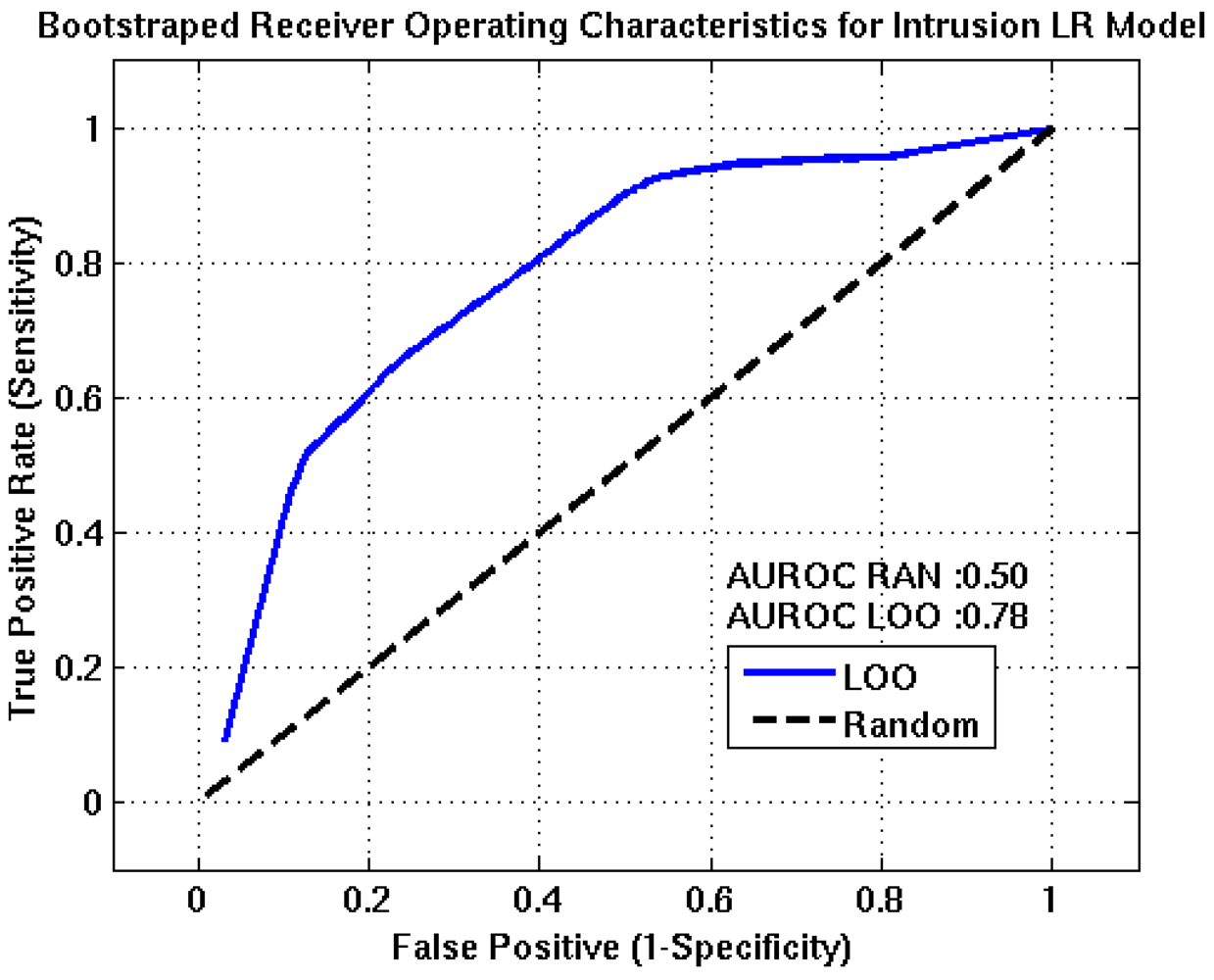
ROC curves for the intrusion, eruption, and intensity event tree nodes are shown in
Figure 5,
Figure 6,
Figure 7. In each plot, the blue line represents the nodes forecasting capability and the black line is the ROC resulting from randomly guessing an outcome. Optimum detection thresholds for each stage of the algorithm are determined from the point on the ROC curve that is closest to the point of perfect classification (0,1), which represents the best trade-off between the TPR and FPR. AUROC estimates for the intrusion, eruption, and intensity nodes are 0.78, 0.81, and 0.80, respectively. These results suggest the algorithm has good forecasting capabilities.
Figure 5.
Receiver Operating Characteristics for the intrusion event tree node. The AUROC value of approximately 0.78 suggests this node will have fair to good predictive capabilities. TPR, FPR, accuracy, and precision estimates of 71%, 29%, 71% and 85% are obtained at the optimum detection threshold, (0.91).
Figure 6.
Receiver Operating Characteristics for the eruption event tree node. The AUROC value of approximately 0.81 suggests this node will have fair to good predictive capabilities. TPR, FPR, accuracy, and precision estimates of 75%, 21%, 78%, and 74% are obtained at the optimum detection threshold, (0.47).
Figure 7.
Receiver Operating Characteristics for the intensity event tree node. The AUROC value of approximately 0.80 suggests this node will have fair to good predictive capabilities. TPR, FPR, accuracy, and precision estimates of 73%, 19%, 78%, and 70% are obtained at the optimum detection threshold, (0.21).
2.7. Algorithm Implementation
Block diagrams highlighting the functionality of the forecasting algorithm are shown in
Figure 8,
Figure 9. Once the process is initiated at a selected volcano, it searches all available monitoring and modeling data for outliers on a day-by-day basis. As data are fed into the algorithm, the user has the option to use the information to model the source of an event. Once the source has been determined, the modeling input parameter (
XMM ) is set to 1 if the unrest is the result of a magmatic intrusion or 0 otherwise. In addition, the algorithm provides a mechanism for a human analyst to override any of the automated results. This allows the analyst to introduce information that may not have been accounted for in the algorithm’s decision making process (e.g., personal experience or information not included in the training data).
Figure 8.
Schematic diagram showing the data flow to and from the forecasting algorithm.
Figure 8.
Schematic diagram showing the data flow to and from the forecasting algorithm.
Upon the detection of unrest, the algorithm’s trigger state vector transitions from 0 to 1. While in the trigger state, data corresponding to the appropriate explanatory variables is routed directly to nodes 2–5 for a user specified number of days. During this time the algorithm produces probability estimates for each node, a daily color coded hazard declaration, an unrest severity estimate, and a vent location probability map. Once the specified number of days has been reached, the trigger states returns to 0, and outlier detection is reinitialized.
Figure 9.
Internal functionality of the forecasting algorithm, where gray indicates processes internal to the algorithm, blue represents external data sources, and green identifies products.
Figure 9.
Internal functionality of the forecasting algorithm, where gray indicates processes internal to the algorithm, blue represents external data sources, and green identifies products.
The logistic models can be recalibrated upon the introduction of new samples into the training dataset. Once the models have been redefined and validated, the old models are replaced, and the new functionality is instantly available at all sites being monitored. This guarantees that all forecasting results are derived from the most recent set of logistic models.
4. Comparisons Between Algorithms
The results generated by the VEFA are compared with those derived from the BETEF v2.0 application. The BETEF tool was developed by Warner Marzocchi, Laura Sandri, and Jacopo Selva of the Istituto Nazionale di Geofisica e Vulcanologia (INGV) and is freely available via the internet. It employs the statistical processing methodology described in [
7,
9]. To use the tool, unique statistical models must be developed for each volcano being monitored. This means each instance of the application uses a set of assumptions and statistical models that are valid only for a specific volcano. These models are non-transportable and have no defined false positive rate or optimized detection threshold. All model weighting coefficients and detection thresholds used by this application are selected subjectively by the user at the time of their development.
The models used for each example were trained using monitoring and modeling data acquired from the most recent unrest episode preceding the event under test. Modeling results (XMM ) were included in the BETEF training set to determine their influence on its forecasting capability. Since eruption history is built directly into the BETEF model during the design process, the XERH parameter is not required as a real time input. Weighting coefficients for all BETEF input parameters (XNE, XCSM , XMM , and XDAYS) were set to 1. All VEFA and BETEF forecasts are based on the same input data to ensure the comparability of results. The median value of the BETEF forecast is used for comparison purposes in all examples shown below. Error estimates were excluded from the comparisons since they are large and typically span the entire probability range.
Forecasts for Grimsvötn and three other volcanoes were compared. The additional volcanoes are located in the western portion of North America and frequently exhibit varying forms of unrest. Okmok is an active shield volcano located on the northern portion of Umnak Island in the center of the Aleutian Arc. Comparison forecasts precede Okmok’s 2008, VEI 4, eruption. Mount Saint Helens is an active stratovolcano that is situated in the Cascade Mountain Range in the southwestern section of Washington State and last erupted in 2004. Forecasts for Mount Saint Helens are generated over a period of seismic activity in February 2011 that was not due to volcanic unrest. The Yellowstone caldera is located in the Snake River Valley in the northwestern portion of Wyoming and last erupted several thousand years ago. Forecasts for Yellowstone are derived over an unprecedented episode of volcanic unrest that occurred in late 2010. The outcome of each test event and its associated seismicity level, in terms of low or high, is listed in
Table 5.
Table 5.
Test event outcome for each algorithm stage and associated seismicity level, where 1 or 0 indicates whether the event occurred or not and if seismicity levels were high or low.
Table 5.
Test event outcome for each algorithm stage and associated seismicity level, where 1 or 0 indicates whether the event occurred or not and if seismicity levels were high or low.
| Volcano | Intrusion | Eruption | Intensity (VEI>1) | High Seismicity |
|---|
| Grimsvötn | 1 | 1 | 1 | 1 |
| Mount Saint Helens | 0 | 0 | 0 | 0 |
| Okmok | 1 | 1 | 1 | 0 |
| Yellowstone | 1 | 0 | 0 | 1 |
Intrusion forecast comparisons for each example are shown in
Figure 17A–D. Intrusion probability estimates for the Grimsvötn and Yellowstone episodes are in very good agreement with one another. However, both of these episodes have a significant amount of associated seismicity which is likely driving the BETEF’s predictions. There are substantial differences between the forecasts for Okmok and Mount Saint Helens. In both cases, the results provided by the VEFA are driven by source modeling results since there is little seismicity associated with these episodes. The supplied modeling information does not appear to influence the BETEF forecasts for Okmok and Mount Saint Helens.
Figure 17.
Intrusion probability comparisons for selected episode days, where each time sample is highlighted with a circle and the VEFA and BETEF results are shown in blue and red. (A) Grimsvötn 2011; (B) Mount Saint Helens 2011; (C) Okmok 2008; (D) Yellowstone 2010.
Figure 17.
Intrusion probability comparisons for selected episode days, where each time sample is highlighted with a circle and the VEFA and BETEF results are shown in blue and red. (A) Grimsvötn 2011; (B) Mount Saint Helens 2011; (C) Okmok 2008; (D) Yellowstone 2010.
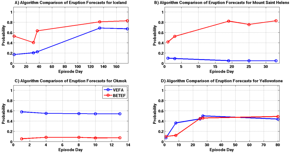
Eruption forecast comparisons are shown in
Figure 18A–D. Forecasts generated for the Grimsvötn and Yellowstone episodes are fairly similar. However, this agreement is again most likely due to the high levels of seismicity produced by these episodes. The large difference between the Okmok and Mount Saint Helens forecasts is still observed, where the results differ on average by 0.6 and 0.7, respectively. This discrepancy is likely due to the lack of seismicity associated with these episodes and the VEFA’s ability to properly assimilate source modeling information.
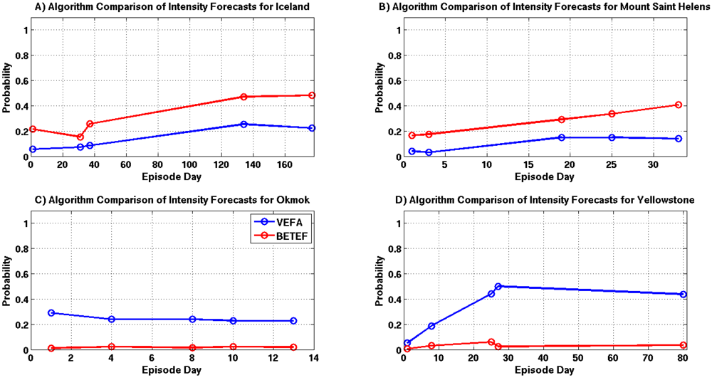
A comparison of eruption intensity estimates are shown in
Figure 19A–D. Forecasts for the Yellowstone episode are significantly different, while the results for Grimsvötn, Okmok and Mount Saint Helens show only small differences. The discrepancy in the Yellowstone forecasts are likely due to the VEFA’s knowledge of the source and the high levels of seismicity associated with this episode.
Figure 18.
Eruption probability comparisons for selected episode days, where each time sample is highlighted with a circle and the VEFA and BETEF results are shown in blue and red. (A) Grimsvötn 2011; (B) Mount Saint Helens 2011; (C) Okmok 2008; (D) Yellowstone 2010.
Figure 18.
Eruption probability comparisons for selected episode days, where each time sample is highlighted with a circle and the VEFA and BETEF results are shown in blue and red. (A) Grimsvötn 2011; (B) Mount Saint Helens 2011; (C) Okmok 2008; (D) Yellowstone 2010.
Figure 19.
Intensity probability comparisons for selected episode days, where each time sample is highlighted with a circle and the VEFA and BETEF results are shown in blue and red. (A) Grimsvötn 2011; (B) Mount Saint Helens 2011; (C) Okmok 2008; (D) Yellowstone 2010.
Figure 19.
Intensity probability comparisons for selected episode days, where each time sample is highlighted with a circle and the VEFA and BETEF results are shown in blue and red. (A) Grimsvötn 2011; (B) Mount Saint Helens 2011; (C) Okmok 2008; (D) Yellowstone 2010.
5. Summary and Conclusions
An algorithm that forecasts volcanic activity using an event tree analysis system and logistic regression has been developed, characterized, and validated. The suite of logistic models that drive the system were derived from a geographically diverse dataset comprised of source modeling results, monitoring data, and the historic behavior of analog volcanoes. This allows the algorithm to simultaneously utilize a diverse set of information in its decision making process. A bootstrapping analysis of the training dataset allowed for the estimation of robust logistic model coefficients. Probabilities generated from the logistic models increase with positive modeling results, escalating seismicity, and high eruption frequency. The cross validation analysis produced a series of ROC curves with AUROC values in the 0.78–0.81 range, indicating that the algorithm has good forecasting capabilities. In addition, ROC curves also allowed for the determination of the false positive rate and optimum detection threshold for each stage of the algorithm.
Modeling results had a significant influence on the probability estimates for the intrusion and eruption nodes and a moderate effect on the intensity node. Logistic functions illustrated in
Figure 2,
Figure 3,
Figure 4 show the influence of modeling information on probabilities decreases between nodes 2, 3, and 4. This result makes sense, because the presence of fluid motion alone does not guarantee escalating volcanic activity. Probability estimates for node 2 should be significantly higher with positive modeling result, since its function is to forecast the presence of fluid motion. However, there is no guarantee an eruption will occur in the presence of fluid motion. Furthermore, the intensity of an eruption is a function of the fluid’s chemical composition, accumulation rate, and amount pressure exerted on its storage vessel. Thus the degradation of the modeling results influence on the probability estimates generated by later nodes is consistent with eruption mechanics.
A comparison of the performance between the VEFA and BETEF further illustrates the power of using source modeling information to produce short-term intrusion and eruption forecasts. Source modeling data significantly enhanced the VEFA’s forecasting capabilities, especially in situations where little or no associated seismicity exists. This point is confirmed by the differences in the BETEF and VEFA intrusion and eruption forecasts for Okmok and Mount Saint Helens. In both cases, the VEFA leveraged source modeling information to confirm or deny the observed unrest was the result of fluid motion. While the BETEF was also given this information during the development and evaluation of its statistical models, it was unable to make the physical connection between the input data and the source of the unrest. Comparison results suggest that a static suite of empirical statistical models derived from a geographically diverse and sparse dataset are transportable and can compete with, and in some cases outperform, non-transportable empirical models trained exclusively from site specific information. This assessment is supported by comparison results showing that the VEFA forecasts are more consistent with the actual outcome of the test events listed in
Table 5.
To the best of our knowledge, this is the first time logistic regression is used to forecast volcanic activity. Furthermore, the derivation of optimized detection thresholds allowed for the quantification of the USGS hazard levels and the determination of an associated false positive rate. This was made possible by the data contained in the volcanic unrest database constructed exclusively for this research. The incorporation of source modeling data into the event tree’s decision making process has initiated the transition of volcano monitoring applications from simple mechanized pattern recognition algorithms to a physical model based system. This paper shows the VEFA has potential for forecasting volcanic activity at various locations throughout the world. Moreover, it can potentially aid civil authorities in determining the proper response to an impending eruption and can be easily implemented by a NVEWS. It should be stressed, however, that this algorithm is meant to assist and not replace the volcanologist in assessing the potential hazard associated with volcanic unrest episodes. Its results should be weighed carefully against a scientist’s personal experience and all other available information. It must also be stressed that low probability of occurrence means the event is unlikely, but not impossible. There will be situations where an unlikely event will occur.
Future work will focus on expanding the training dataset. Emphasis will be placed on identifying additional explanatory variables that can further enhance the predictive power of the algorithm. The Earth Observatory of Singapore, Nanyang Technological University, is leading a research initiative to develop a global volcanic unrest database referred to as WOVOdat [
72]. This database will contain observations from various monitoring technologies and source modeling results from volcanoes all over the world. However, this database is under construction and is not yet open to the public. Once available, each of the logistic models will be redefined to exploit this diverse and comprehensive database. In addition, comparisons with other decision making techniques such as Classification and Regression Tree (CART) analysis will also be performed.


 , whereas the probability of an eruption occurring at a given volcano is estimated by P(Θ1) P(Θ2) P(Θ3).







 samples within 1.15 km of each epicenter are set to 1. Due to the absence of modeling information, maps for days 1 and 37 show probable vent locations scattered over the Vatnajökull icecap. Initially, the search area spans 2979 km2, J = 7,094,495, and all
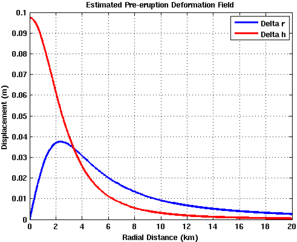
  = 0. Modeling results shown in Figure 11 suggest that the deformation source is located approximately 3.33 km below the caldera center and has an isotropic radiation pattern with a 17 km radius. This information provides the justification to quantitatively constrain the PDF to a square search area spanning 1156 km2, reduce J to 2,788,920 probable locations, and set all
  = 1. As seismic activity accumulates over time, the spatial PDF begins to highlight a preferred vent location. Maps computed for day 134 and day 177 show that the most likely area for vent formation is in the south and southeastern portions of the caldera. Grimsvötn’s 2011 eruption occurred in the southern section of the caldera with a VEI greater than 1.0 [71].

