Abstract
We present a complete, end-to-end computer-aided detection (CAD) system for identifying lesions in the colon, imaged with computed tomography (CT). This system includes facilities for colon segmentation, candidate generation, feature analysis, and classification. The algorithms have been designed to offer robust performance to variation in image data and patient preparation. By utilizing efficient 2D and 3D processing, software optimizations, multi-threading, feature selection, and an optimized cascade classifier, the CAD system quickly determines a set of detection marks. The colon CAD system has been validated on the largest set of data to date, and demonstrates excellent performance, in terms of its high sensitivity, low false positive rate, and computational efficiency.
1. Introduction
Colorectal cancer is the second leading cause of cancer related death in western countries and the third most common human malignancy in the United States [1]. Most colorectal cancers arise from pre-malignant polyps in the colon that develop into cancer over time. The progression from polyp to cancerous lesion takes more than ten years for most patients. Because of this slow growth rate, colon cancer screening [2] is an effective method for polyp detection, and subsequent removal reduces the risk of colorectal cancer by up to 90 percent [3]. Colonoscopy, the endoscopic examination of the colon using a flexible video camera, is the standard approach to colorectal screening; however, in recent years there has been much interest in CT Colonography (CTC), which uses CT images of the cleansed and insufflated colon [4]. Polyps can then be detected by a clinical reader who examines the CT data using advanced visualization software that provides both 3D endoluminal views of the colon as well as 2D multi-planar reformatted slices.
Compared to optical colonoscopy, CTC has the advantages that it affords rapid imaging of the entire colon, is less invasive, and has virtually no risk of perforation of the colon. Clinical studies suggest CTC can provide similar detection performance as colonoscopy but has a reduced risk of complication [5]. Although CT imaging typically exposes the patient to 5-8 mSv of radiation, this exposure is comparable to a few years of natural background radiation, and therefore should not be a significant component of the consideration to use CTC for polyp screening [6].
The lesion size is directly related to the likelihood of malignancy [2]. Diminutive polyps, i.e., those less than 6 mm in size (measured in the single largest dimension of the polyp head) are not thought to confer significant clinical risk. Small polyps in the 6–9 mm range are typically pre-cancerous and are of interest for reporting during the exam; such polyps may be flagged for surveillance or surgical removal. Lesions 10 mm and larger confer higher clinical risk, as 10–25% of these lesions may exhibit malignancy.
Although CTC has been demonstrated to be an effective colorectal screening approach [7], it is possible for the clinical reader to fail to detect lesions, due to the large quantity of data generated (typically 800–2000 images per patient). Computer-aided detection (CAD) software assists the clinical reader by automatically analyzing the CT data and highlighting potential lesions. CAD may detect lesions that would have otherwise been missed by the reader, and furthermore may give the reader more confidence that lesions were not missed during the read. It has been demonstrated that the use of CAD leads to improvements in reader performance (at all levels of experience) in detecting lesions in CTC data [8, 9].
An important challenge in developing CAD software is robustness, as the CAD must work effectively across a wide range of operating conditions. Patients may have different preparations, including the type and degree of cathartic cleansing, the use or lack thereof of liquid and fecal tagging agents, and level of insufflation of the colon during scanning. Different imaging hardware (from various manufacturers) or imaging protocols (slice thickness, tube current, patient positioning, etc.) may be employed. Populations may have differences as well, coming from different institutions, and may be symptomatic or asymptomatic. Another, often overlooked issue relates to the computational resources required to run the CAD. Given the vast quantity of data to be analyzed, the processing must be fast in order to optimize the clinical workflow, and additionally be memory efficient to be practical when running in conjunction with advanced visualization software.
1.1. Related work
Given the clinical importance of polyp detection, the subject of CTC-CAD has received considerable interest in the literature. Since there is no universally agreed upon set of a data and evaluation methodology for comparing CAD systems, clear and accurate comparisons between different CAD systems are not possible. However, a summary of many recent CTC-CAD systems, presented in Table 1, does provide a picture of the state-of-the-art in CTC-CAD. In the table, where possible, we list the data sources (number of centers from which the data came), training and testing data sets (in terms of patients), per-polyp sensitivity, false positives (FPs)/volume, and runtime when executed on a new volume (note different computers and CPUs are used so exact comparisons are not available). More statistical confidence would be attributed to CAD systems tested on larger sets of data. For the reasons mentioned earlier, in the table we focus on the detection of lesions 6 mm and larger. Note that each patient is scanned twice; once in a prone position and once in a supine position. Throughout the paper, we report FPs/volume, as is the convention in CTC.

Table 1.
CTC-CAD results reported in the literature. From left to right: columns refer to the reference, number of different data centers from which the data came, number of patients used in training, number of patients used in testing, per polyp sensitivity, false positives per volume (per patient false positive rates can be determined by multiplying the per volume false positive rate by 2), and algorithm runtime per volume.
| Reference | Data cen | Train | Test | Per-polyp sens. | FP / vol. (or 2x per patient) | Runtime / vol. |
|---|---|---|---|---|---|---|
| Yoshida et al. [10] | 71 | 71 | 90% (5mm+) | 1 | ||
| Paik et al. [11, 12] | 2 | 8 | 35 | <35% (5mm+) | 2.5 | |
| Summers et al. [13] | 3 | 394 | 792 | 61.3% (6mm+) | 3.95 | 10 min |
| Bogoni et al. [14] | 2 | 88 | 62 | 90.5% (5mm+) | (3 median) | 4 min |
| Jerebko et al. [15] | 96 | 72 | 94% (5mm+) | 4.3 | ||
| Bhotika et al. [16] | 42 | 81.6% (>6mm) | 5.2 | |||
| Tu et al. [17] | 117 | 35 | 92% (6mm+) | 5.8 | ||
| Kim et al. [18] | 15 | 35 | 77.1% (6mm+) | 3.1 | ||
| Dundar et al. [19] | 2 | 169 | 201 | 86% (n/a) | 5 | 4 min 43 sec |
| Qiu et al. [20] | 2 | 10 | 98 | 100% (n/a) | 3 | several minutes |
| Sundaram et al. [12] | 2 | 35 | 76% (5mm+) | 2.5 | 2 min 20 sec | |
| Suzuki et al. [21] | 1 | 10 | 73 | 96.4% (5mm+) | 0.55 | |
| Li et al. [22] | 3 | 394 | 793 | 77.4% (6mm+) | 2.91 | |
| Liu et al. [23] | 3 | 395 | 791 | 75% (6 - 9 mm) | 2.5 | |
| van Ravesteijn et al. [24] | 4 | 86 | 307 | 85 - 100% (6mm+) | 4-6 | |
| This paper | 8 | 180 | 3106 | 90.1% (6mm+) | 4.7 (3 median) | 1 min 23 sec |
Progress on the problem of CTC-CAD started with the pioneering work of Vining et al. [25], who identified polyps as an abnormal thickening of the colonic wall. Subsequent work by others focuses primarily on use of curvature as a mechanism for detecting polyps. The work of Summers et al. [13] utilizes mean curvature computed at voxels on the mucosal surface. Yoshida and Nappi [26] apply shape index and curvedness [27] to find initial candidates, which are then clustered and classified using quadratic discriminant analysis, whereas Kim et al. [18] rely on eigenvalues of the Hessian matrix. Instead of computing curvature information on the voxel grid, Sundaram et al. [12] apply a geometry processing approach directly on a mesh-based representation of the colon. Van Ravesteijn et al. [24] use the second principle curvature in a differential equation that is solved explicitly on a mesh or implicitly on the image grid to identify polyp candidates. Jerebko et al. [15] extend [14] by analyzing the symmetry of curvature patterns of raised objects in the colonic lumen. Others have deduced analytic shape models [16] to approximate local geometry of the colon, or measure the degree to which back-projected surface normals overlap [11, 28]. Still others have analyzed texture patterns of electronic biopsy images of the flattened colon [20].
In addition to advances in initial detection of polyp candidates using various intensity and morphologic features, much progress has been made in classification. Initial work in colon CAD focused on applications of relatively simple machine learning algorithms to differentiate patterns of lesions from non-lesions. Recent work by Dundar et al. [19] designs optimized cascade classifiers using an AND-OR framework to minimize an overall objective function. Suzuki et al. [21] extend Yoshida et al.’s approach [26] with a massive-training artificial neural network to further reduce false positive findings, showing promising results. Liu et al. [23] apply manifold learning techniques such as diffusion maps and local linear embedding for dimensionality reduction in conjunction with a support vector machine. Recently in the computer vision and machine learning literature, there has been much interest in Adaboost, which forms a strong classifier from a set of weak learners and is less sensitive to overfitting than other classifiers. Tu et al. [17] design a probabilistic boosting tree composed of Adaboost classifiers for automatic polyp detection without requiring colon segmentation. Ideally, the data used to develop and validate the CAD will comprise a diverse set of CTC scans that fully characterize the populations, patient preparations, CT scanners, and imaging protocols in clinical practice. Naturally, data used for testing the CAD should be independent of the data used to train the system.
1.2. Our contribution
In this paper, we present a complete, end-to-end CAD system for the detection of lesions (polyps or cancers) in CTC. Our system has been designed to offer robust performance in the presence of variations in image data and patient preparation. It has been developed and validated using data from eight different institutions, with different imaging hardware (Siemens, GE, Philips, Toshiba), scanning protocols and patient preparation. In addition, the CAD system has been optimized for computational efficiency by making use of efficient 2D and 3D processing, software optimizations, multi-threading, feature selection using information-theoretic techniques, and an optimized cascade classifier. Clinical results on the largest ever colon CAD trial (over 3000 patients) demonstrate per-polyp sensitivity of and average (3 median) false positives per volume. In addition, the CAD runs in 1 minute and 23 seconds (average) on a standard quad-core 2.4 GHz processor while requiring at most 150 MB of RAM regardless of the number of images in the volume.
The rest of the paper is organized as follows. In Section 2 we present an overview of our CAD system, followed by more detailed descriptions of the major components in Section 3, Section 4, Section 5 and Section 6. In Section 7 we present experimental results demonstrating the effectiveness of our approach. Finally, in Section 8 we conclude the paper and discuss future work.
2. CAD System Overview
A block diagram of our colon CAD system, illustrating its major components, appears in Figure 1. Starting with a CT image, an automatic colon segmentation algorithm first identifies voxels representing the colon, producing a region of interest for subsequent processing. Next, a candidate generation step analyzes the mucosal surface, finding and grouping, as 3D regions, protrusions into the lumen. For each region, statistical features are calculated and used in a cascade Adaboost classifier. The calculation of features is interleaved with the classifier stages for computational efficiency, as will be described in more detail below. The final CAD marks are then presented to the reader.
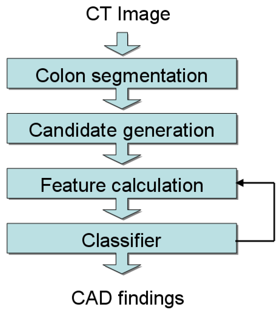
Figure 1.
Block diagram for CAD system overview.
3. Colon Segmentation
The colon segmentation step produces a binary colon mask that represents the voxels corresponding to the colon; a block diagram of this subcomponent is provided in Figure 2. When the scan is performed, the patient’s colon is distended with carbon dioxide (or air), which appears very dark in the CT image. Ideally the colon is a singly-connected air-filled region as a result of the distension, however, collapsed segments are possible. Additionally, the patient may have been administered oral contrast agents for tagging liquid and solid residues in the colon. In the CT image, these appear as very bright regions (typically with Hounsfield units (HU) ). The colon segmentation is designed to be robust to these complicating factors.
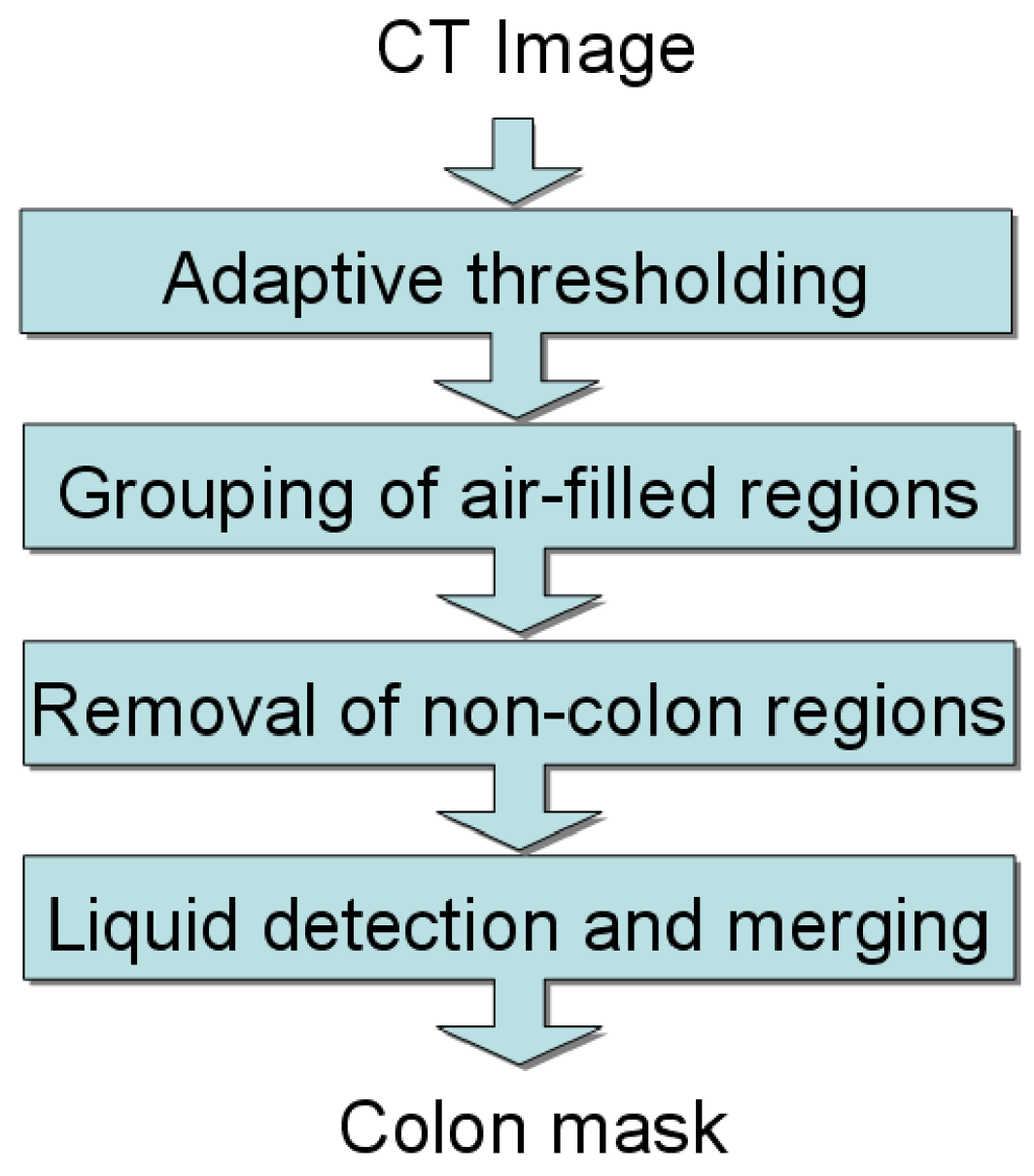
Figure 2.
Block diagram for the colon segmentation.
We note that all steps in our colon segmentation process the image (and resulting segmentation mask, stored on the hard drive) in consecutive order along axial slices, with only a few slices loaded into memory at any given time. Such out-of-core [29] processing provides an effective way to achieve memory-efficiency when dealing with large data sets.
3.1. Adaptive thresholding and grouping
The first step of our colon segmentation approach is an adaptive thresholding of the image, separating it into air and non-air voxels. Following [30], the threshold is computed adaptively based on the image histogram using an entropy-based measure, and clipped to ensure it is within the range . After thresholding, all air voxels are foreground and all non-air voxels are background in the segmentation mask, as demonstrated in Figure 3(a). Next, foreground voxels are grouped into disjoint segments and labeled based on their 3D connectivity. While voxels corresponding to the air-filled colon are easily found as a result of this thresholding, often other air-filled anatomies like the lungs, small bowel, and stomach, as well as the air outside the body are included. Removal of these non-colon segments is described in the next subsection.
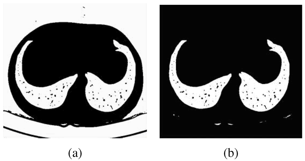
Figure 3.
Thresholding (a) and outer air removal (b) demonstrated on an axial slice that includes the lungs.
3.2. Removal of non-colon segments
At this stage, the air outside the body is easily discarded from the mask by detecting the largest connected component touching the image border. An example after this operation is shown in Figure 3(b). From the remaining voxels, a bounding box (used later) is determined and encloses the body of the patient. Next, the remaining 3D regions are analyzed in order to separate the colon from the remaining non-colon regions. Care is taken to design the non-colon segment removal for high sensitivity; that is, it is preferable to include a small non-colon region than to remove a colon region. Although this may later lead to false positive CAD marks outside the colon, such CAD marks are easily dismissed by the clinical reader and significantly less important than false negatives in the colon.
The lung detection and removal algorithm analyzes 2D axial slices, moving from the top of the volume down towards the rectum. Lung detection is primarily based on two features of the lungs:
- The lungs contain many small blood vessels, which appear as small “holes” in the segmentation mask.
- The lungs are continuous anatomic regions and therefore should have significant overlap in adjacent axial slices.
On a 2D slice, a small region is considered to be a hole if it is contained within a labeled region and consists of or more connected background pixels; holes appear as small dark regions as shown in Figure 3 (b). A 3D labeled region is considered to be lung if it contains at least holes. and were set to 2 and 10 experimentally. Once the lung regions are detected on each 2D slice, the amount of overlap on adjacent slices is determined. Starting with the topmost slice in the volume, the degree of overlap of the ith labeled region is determined with lung regions on the next slice, that is,
where is a threshold set as . If the above condition holds, is removed from the segmentation mask.
The stomach is located near the lung area and near the transverse colon and often appears as a large hollow object in the CT scan. A 3D labelled object is identified as stomach if it only appears in the top (as measured in the z-direction) one third of the volume. After detection, the stomach is removed from the segmentation mask.
Small bowel can be detected and removed from the segmentation mask based on the following observations:
- Small bowel segments tend to have smaller volume than large bowel segments.
- In a coronal view, the colon frames (surrounds) the small bowel, as shown in Figure 4.
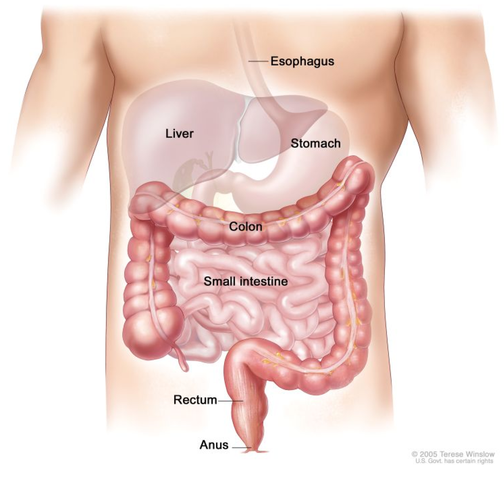
Figure 4.
Illustration of the small bowel (intestine) and colon. Notice that the small bowel is framed by the colon in this coronal view. Public domain image courtesy of the U.S. government.
Based on these observations, we first remove any segment below , which eliminates much of the small bowel. However, when the colon is sufficiently distended, some small bowel segments may still remain in the segmentation mask. A second filter is applied using the bounding box , which is reduced mm on all six sides, forming a new bounding box . Any segment with bounding box that is completely contained in is removed from the segmentation mask.
3.3. Liquid detection and merging
In CTC, fecal materials are often tagged by orally administered contrast agents that are opaque to X-rays, appearing as the bright regions in the colon in Figure 5 (a). These materials can assist in differentiating residual solid stool versus tissues like polyps, since the resulting intensity in the CT image for the agent is high, usually in the range . In this step of the algorithm, the liquid contrast agent is detected and merged with the segmentation mask. Liquid is detected primarily using three features:
- The liquid has a high intensity.
- The liquid is below an air-filled region.
- The interface between the liquid and air is planar.
This function performs a simple thresholding in the original image using a high threshold . The voxels above the threshold are labeled into distinct regions. For each region, an analysis is done on each axial slice to determine its flatness. A bright region is considered flat in a 2D slice if of its pixels have the same y (corresponding to the axis of gravity) value. is determined as , where is the width of the region’s bounding box. To fill the partial volume between the air and the liquid region, rays are cast from the liquid region upwards along the y axis towards the air, and the voxels in between are added to the segmentation mask, as demonstrated in Figure 5 (b).
After this step, the colon segmentation is complete and the foreground voxels in the mask represent the colonic region of interest used in subsequent processing. A sample colon segmentation appears in Figure 5 (c).
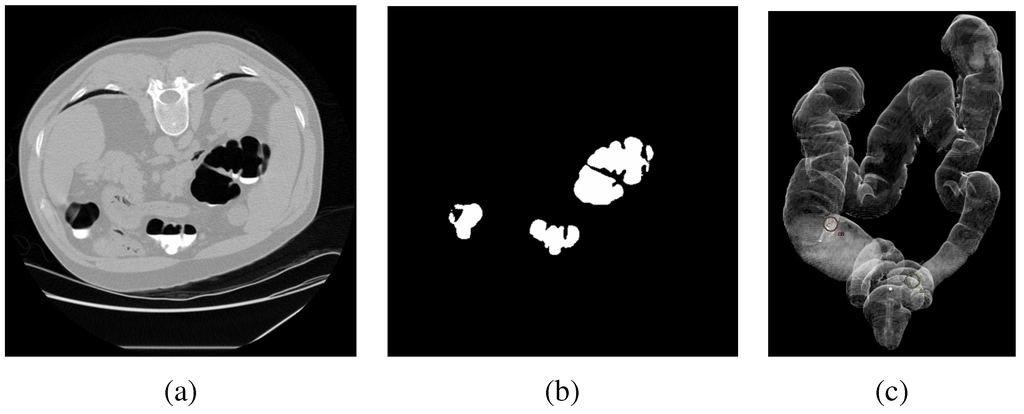
Figure 5.
Original slice (a) and colon segmentation after liquid detection and merging (b). Final colon segmentation, with overlaid CAD marks (c).
4. Candidate Generation
Candidate generation identifies, using the colon segmentation, 3D regions (also called raised objects in this paper) that protrude into the colon lumen. As with the colon segmentation, all processing is done on a slice-by-slice basis, traversing the volume axially.
4.1. Critical point detection
For each 2D slice, each point along the contour of the colon is analyzed in terms of its convexity. Raised objects will have at least one concave point and should be accompanied by two convex points, on either side of the concave point, where the object is attached to the surface. Examples are shown in Figure 6. From this convexity determination, raised objects are extracted from the image.
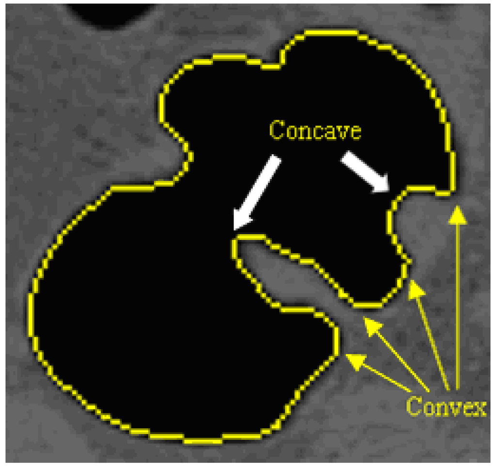
Figure 6.
Convexity analysis along a 2D contour of the colon segmentation.
First, an angle is computed each point along the contour based on a chain code [31] using an eight neighborhood. Due to the discrete nature of the data, angles are naturally quantized to angles. To provide robustness to noise, a lowpass Gaussian filter with standard deviation is applied to smooth the angles. Then, each point is classified as convex, concave, or smooth, using the following equation:
where . Critical points are those for which this classification changes; i.e., points where the convexity/concavity transitions. The concave regions of the contour are identified, and the convex critical points defining the start and end points of the raised object are detected. A line between the two critical points is drawn, and the 2D region defined by this line and the concave part of the contour is stored as a 2D candidate. A schematic illustration is provided in Figure 7.
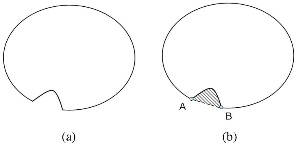
Figure 7.
Schematic illustration of a 2D slice (a) for detection of critical points A and B, as well as the candidate region (rendered with gray stripes) shown in (b).
4.2. Formation of 3D regions
After all axial slices within the bounding box of the colon have been processed to generate 2D candidates, a grouping algorithm is run to produce 3D candidate regions. 2D candidate regions are grouped if they overlap and their core regions also overlap. The core is the central part of a region for which all points have a boundary-seed distance greater than , where is the maximum value of the distance transform in the region. The use of the core allows for the separation of polyps from folds in cases where the two objects are attached. The output of this step is a 3D candidate region.
Our candidate generation method [32] has several advantages. First, by processing the data in a slice-by-slice fashion, only a small subset of 3D volume is loaded at any time, thus achieving memory efficiency. In addition, the detection of concave regions is independent of the size of the raised object; thereby enabling detection of raised objects of any size. The candidate generation is designed to detect as many true positives as possible. However, it may include many false positive regions (in particular, folds), which are subsequently removed by our classifier using region-based features, discussed next.
5. Region-Based Features
While the candidate generation produces a set of 3D candidate regions that may potentially be lesions, at this stage in the processing there are typically thousands of candidates. A set of descriptive features that characterize each region are calculated and used in a cascade classifier, described in the next section. We note that each 3D candidate is a small subvolume of the original CT image, therefore, all feature calculations (and subsequent classification) is performed on this subvolume, achieved with low memory usage. We now describe our features, which have been categorized into the following classes: intensity, differential geometry, texture, volume, and other features, described below.
5.1. Intensity features
Statistical features of the image intensity are useful in discriminating between true positives and false positives (typically folds, residual stool, etc.). For example, tagged stool tends to have a very high intensity. Untagged stool tends to have small pockets of air, which results in a higher CT variance for the voxels in the region. Using the set of voxels in the 3D region, we compute the following six intensity features:
- Mean, standard deviation, maximum
- Entropy and skew of histogram
- Average correlation of intensities from adjacent 2D slices
5.2. Differential geometric features
Polypoidal lesions may have a hemispherical shape or contain sections of their shape that are locally spherical. As a result, features derived from curvature of the mucosal surface are often highly discriminative, especially when distinguishing polypoidal lesions (part spherical) from folds (part cylindrical, or ridge-like). Differential geometric features can be computed from an explicit representation of the mucosal surface [12] or implicitly on the isosurface around a voxel [33, 34]. Following the example of [10], for each voxel in the region, we compute the volumetric shape index (SI) and curvedness (CV), defined as
where and are the principal curvatures, computed directly from the image intensities. Every distinct shape, except for the plane, corresponds to a unique shape index. Most importantly for colon CAD, spherical shapes have a high shape index of 1.0, while ridge-like shapes have a lower shape index of 0.75; this enables the discrimination of polyps from folds. The curvedness represents the size of the curved object. For instance, a smaller and larger sphere might have the same shape index but different curvedness values. After computing the shape index and curvedness at each voxel in the region, we then compute the following nine statistical features of the region:
- Mean, entropy, skew, standard deviation, and maximum of shape index
- Mean, entropy, skew, and standard deviation of curvedness
5.3. Gradient concentration features
The degree to which image gradients converge within a region is a discriminative feature for identifying polyps. Following the example of [10, 35], we compute the gradient concentration (GC) and directional gradient concentration (DGC) (see [10] for mathematical details) at each point in the region. Then, we compute the following statistical features using both the GC and DGC, producing 18 total features:
- Mean, min, max, variance, mean of ten highest values, ratio of min and max
- Skew, kurtosis, entropy of histogram
5.4. Texture features
Several authors have recently explored the use of texture features to differentiate lesions from non-lesions [17, 36, 37, 38]. For each region, we perform texture analysis following Laws [39], who forms 2D convolution kernels as outer products of 1D convolution kernels. The 1D kernels we use include
which compose the following 2D convolution kernels: , , , , , , , , . Each slice of the region is convolved with these kernels, resulting in 9 output filterings. For each, we then compute the following statistical features, resulting in a set of 27 texture features:
- Mean, standard deviation
- Entropy of histogram
5.5. Volume features
We compute various volume-based features to characterize the region. Diminutive findings are often identified based on the number of voxels in the region. Since folds typically appear as thin cylindrical structures, they may have a small maximum distance based on a boundary-seeded distance transform [40]. Other features are based on the degree of sphericity of the region. Specifically, we compute:
- Number of voxels in region multiplied by slice thickness
- Maximum value of boundary-seeded distance transform applied to region
- Ratio of actual volume to that of a sphere with the maximal diameter of region
- Number of voxels with shape index multiplied by slice thickness (shape cluster size)
5.6. Other shape features
Some other shape features computed include:
- Region width (maximum diameter)
- Region height
- Ratio of height to width of region
- Elongation, defined as the ratio of eigenvalues derived from the covariance matrix of points in the region.
- Number of voxels with “dot” value (described in detail below) greater than a threshold .
The dot feature we use is based on the dot enhancement approach of [41], originally designed to enhance the objects in an image of a specific shape. For each voxel, the dot value is defined as
where are three eigenvalues of the Hessian matrix calculated from second derivatives of image.
To reduce the effect of the noise and also to take into account different object sizes, multi-scale Gaussian image smoothing is performed prior to the calculation of the second derivatives. Following [41], for objects with diameters in the range to be detected, discrete smoothing scales are calculated as , , where . The maximum dot value calculated among the different scales is chosen to be the final dot value for each voxel in the region. In this paper, Gaussian scales are used. The feature is then the total number of voxels with dot value greater than .
5.7. Other binary features
Finally, some binary features are computed as well:
- Region touching liquid (detected during colon segmentation)
- Region submerged (detected during colon segmentation)
- Region is small (defined as having a width less than 3.5 mm or height less than 1.4 mm)
In total, there are a potential set of 72 unique features that can be used to characterize a region in the CT image. The majority of features have low computational cost, since the 3D regions are typically small subvolumes of the entire scan. However, the gradient concentration, texture features, and dot feature are most expensive, a fact that is used later in designing our classifier.
6. Classification
In this section, we describe our classification methodology, which is based on cascade Adaboost. For efficiency, the first stage of the cascade is based on features that have low computational cost and selected by a feature selection technique.
6.1. Challenge
The candidate generation was designed to keep a high sensitivity, even at the expense of many false positives. As a result, the candidates exhibit a large class imbalance. Therefore, an accurate identification of polyp regions (minority) from the non-polyp regions (majority) is a challenge for a CAD classifier; techniques such as [42] can be used to tackle such problems. Moreover, the features differ in terms of their computational complexity; some are more expensive to compute than others. For efficiency, it is therefore undesirable to compute a full feature set for all candidates when many can be rejected using a reduced set of features that are simple to compute.
6.2. Cascade
A cascade framework of Adaboost was proposed by Viola and Jones [43] to solve the problem of face detection. The cascade is a degenerate decision tree, with each node an Adaboost classifier. A positive result from the first classifier triggers the evaluation of a second classifier, both of which are designed to achieve high detection rates. A positive result from the second classifier triggers a third classifier, and so on. A negative outcome at any point leads to the immediate rejection of the candidate. With the difficulties of a huge number of candidates and features in face detection, the cascade approach can construct simple classifiers which, at the early stages of the cascade, reject the vast majority of negative samples while detecting almost all positive instances, thereby achieving results with significantly reduced computation. Only the difficult samples require more complex features.
A limitation of the cascade framework is that the target of each node (detection rate and false positive rate) has to be chosen manually, and is therefore subjective based on the experience of the developer of the classifier. Unfortunately, in standard cascade implementations, there is no direct relationship between the objective taken at each node and the overall performance. To overcome this, we adopted a cascade optimization method developed by Sun et al. [44], who present a cascade indifference curve, which connects the performance of each node with the overall performance. This leads to an automated cascade with improved overall performance, without requiring a target for each node.
6.3. Adaboost
AdaBoost, introduced by Freund and Schapire [45], is a serial ensemble approach that builds an additive model. At each step of the ensemble construction, the approach adds a new weak learner that can focus on misclassified samples from the previous step by reweighting the training samples (increasing the weights of misclassified examples and decreasing the weights of correctly classified samples). In this way, it forms a strong classifier with a linear combination of weak learners. AdaBoost has shown a strong performance in many applications. In our implementation, weak learners are decision stumps that include a selected single feature and a threshold value that operates on the feature to form a decision boundary between positive and negative class samples.
6.4. Feature selection with mutual information
For the first stage of our classifier, we rely on features that have low computational cost, so that many candidates can be rejected quickly. To select these features from the complete set of low-cost features, we employ the maximum relevance, minimum redundancy (MRMR) technique proposed by [46].
In information theory, mutual information measures the statistical dependency between two random variables. The problem of feature selection can be interpreted as a search for a subset of features that jointly have the largest dependency on the target class (polyps, in our case). The MRMR approach, which extends work from Battiti [47] and Kwak and Choi [48], selects a good subset of features as the one that has a large dependency on the target class. However, a difficulty of estimating multivariate densities accurately makes the computation challenging, especially for continuous features. Instead of seeking maximum dependency, MRMR seeks a subset of features that are maximally relevant on the target class but for which the features within the subset are minimally redundant. It can be formulated as
where D and R represent the relevance and dependence, respectively, and measures the mutual information between feature and the target class c, and measures the mutual information between two features and . In practice, Equation 9 can be implemented incrementally as follows:
The method starts by seeking a single feature that is maximally relevant to target class, and includes in the set . From the remaining features , it then seeks the next feature that is maximally relevant to target class but minimally redundant with features that have been previously selected. The selected feature, along with feature set , forms feature set . This process iterates until the number of features has reached m features, .
6.5. Data and training
The CT colonography data in our experiments consisted of 382 patients (764 CT volumes) of prone and supine volumes collected from 8 institutions. The data is highly diverse. CT images were generated using scanners from all the major manufacturers, including Siemens, GE, Philips, and Toshiba, with 4, 8, 16, 32, and 64 multi-slice configurations, as described in Table 2. KVp ranged from , and exposure ranged from 29–500 mAs. Patients were placed in feet first prone and supine, head first prone and supine, as well as decubitus positions. All subjects were scanned within the last 10 years (1999–2008) and roughly were administered fluid and fecal tagging. When measuring performance of the CAD, the sensitivity is measured per polyp (that is, if a polyp is detected on either or both volumes it is considered a true positive) and false positives are measured per volume, as is the convention in CTC. Per patient false positive rates can be determined by multiplying the per volume false positive rate by 2.

Table 2.
Scanning equipment used to produce the data.
| Manufacturer | Model | Multi-slice configurations |
|---|---|---|
| Siemens | Somatom | 4, 16, 64 |
| GE | Lightspeed | 4, 8, 16 |
| Philips | Brilliance | 4, 64 |
| Toshiba | Aquilon | 16, 32, 64 |
This data was split into two subsets: dataset1, containing 180 patients (360 volumes) for training and dataset2, containing 202 patients (404 volumes) for independent testing. On each slice, the average pixel dimensions were mm by mm, and on this varied set of data, the slice thickness ranged between mm to mm. Dataset1 had 168 polyps mm in size, and 102 polyps mm in size. Dataset2 had 119 polyps mm in size, and 75 polyps mm in size. We randomly divided dataset1 as for training and for validation, which was used to test and adjust the training to maximize performance. We also tested the constructed model on dataset2. For ground truth, three medical experts performed a consensus annotation of the scans.
The training data was randomly divided into for training AdaBoost and for determining the objective performance for each node. The candidate generation algorithm typically produces a few thousand candidates, which are then classified using the 72 features described in the previous section. At the first node of the cascade, a four feature subset was selected by MRMR from the cost-efficient feature set and trained by AdaBoost. These selected features are variance of intensity, shape index cluster size, and mean and variance of shape index. The selected features provide an intuitive meaning for false positive filtering, as described in Yoshida et al.’s paper [26], which applies shape index clustering for candidate generation. After the first stage, any feature may be used by the cascade when required by the classifier.
In testing, the feature calculation is interleaved with the cascade classifier. At any particular stage in the cascade, we only compute the required features. The full set of features is only computed for the regions that are hardest to classify, resulting in computational savings.
6.6. Multi-threading and software optimizations
To achieve further computational efficiency, the CAD system has been multi-threaded using OpenMP pragmas, which are compiler directives for parallelization. Specifically, the features/classifier loop has been multi-threaded, effectively sending a subset of the candidates for classification to each core of the processor. Multi-threading is implemented using #pragma omp parallel for directives, placed immediately above the loop. The directive instructs the compiler to spawn multiple threads of control, where each thread is responsible for a portion of the loop. For example, in a quad-core implementation, it is likely the four threads would be spawned, theoretically resulting in a 4x speedup of the loop; however, the actual speedup is typically less than this due to synchronization and shared memory. The multi-threaded code produces the exactly the same results as the single-threaded version of the code. More information about OpenMP and its specifications can be found at the official website, www.openmp.org.
In addition to multi-threading, we also applied software optimizations to compute the CAD marks quickly, inspired by optimizations for fast boundary-seeded distance transforms [40], labeling [49], and hole detection. Prior to the software optimizations and multi-threading, the system took on average 3 min, 42 seconds to process a volume. After optimization, this time reduced nearly to 1 min, 23 seconds, when tested on a standard quad-core 2.4 GHz processor. As a result of the memory-efficient implementation, the system only requires at most 150 MB of RAM regardless of the number of images in the volume.
7. Results
7.1. Experimental results
A quantitative evaluation of the performance of our CAD has been conducted for the detection of lesions above 6 mm and 10 mm, respectively. As mentioned previously, the testing data includes 202 patients (404 volumes), with 119 lesions above 6 mm and 75 lesions above 10 mm. A CAD mark is considered successful if the point lies within the ground truth annotation. Free-Response Operator Characteristic (FROC) curves plotting the sensitivity vs. false positives appear in Figure 8, showing the detection performance at these two size thresholds. The points along the curve demonstrate the performance after successive stages in the cascade. Although the entire FROC curve is shown, the performance at the operating point available in the commercially available product (Medicsight ColonCAD 4.0) is indicated in the plot. At this point, the CAD system achieves an overall per-polyp sensitivity of (for polyps 10mm and greater) and (for polyps 6 mm and greater), with the same false positives of 4.5 per volume on average. These results are summarized in Table 3.
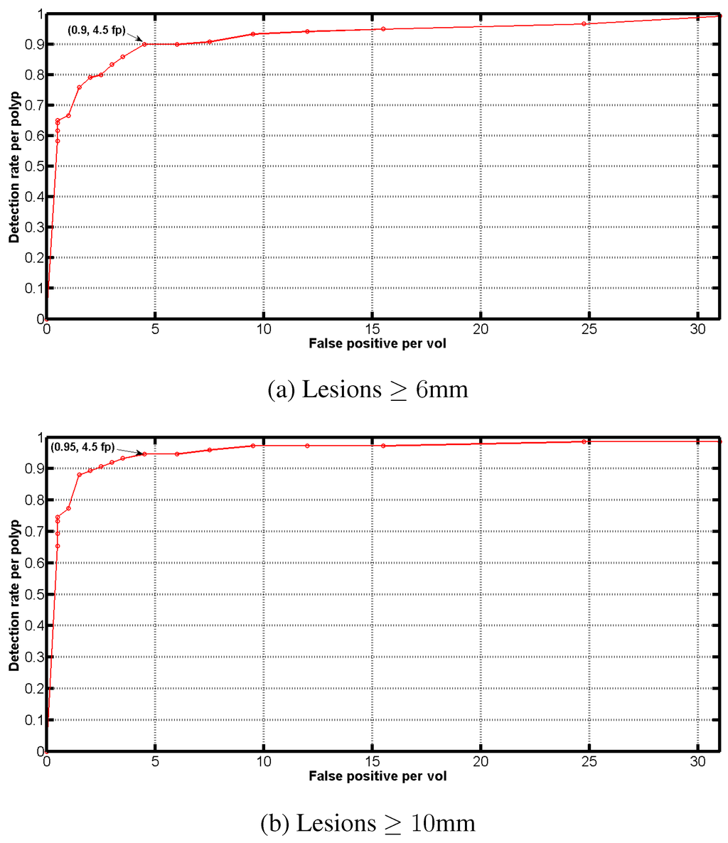
Figure 8.
FROC curves demonstrating CAD performance on independent test data for lesions mm (a) and mm (b).
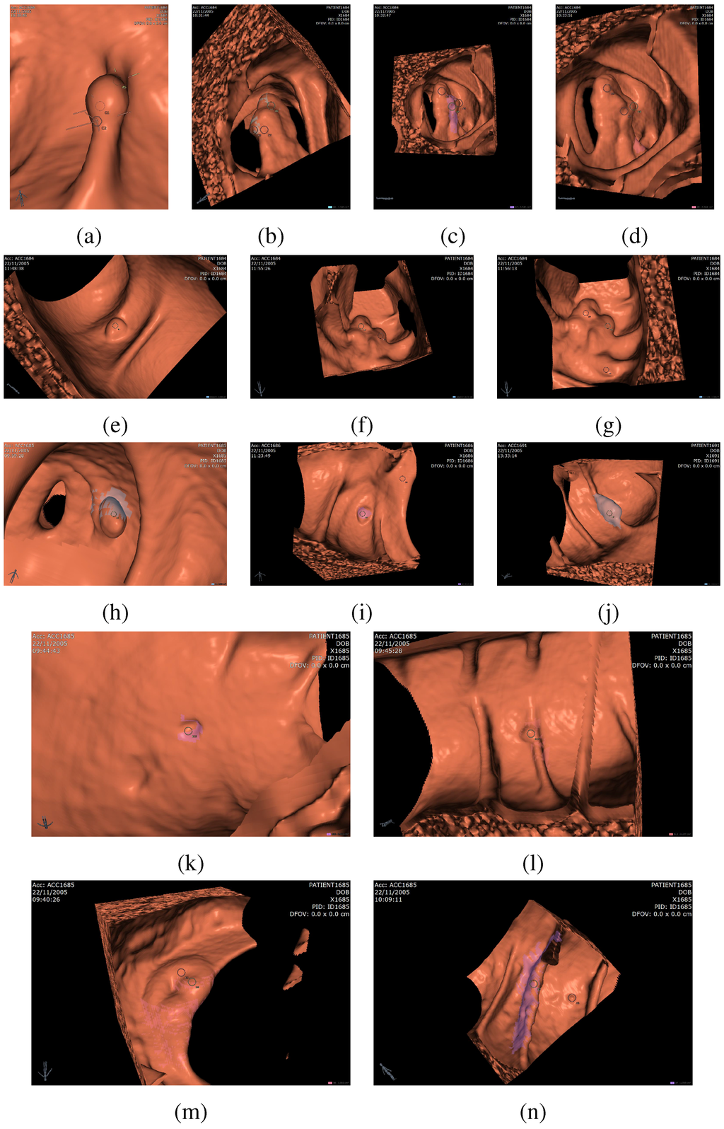
Figure 9.
Examples of detected polyps and false positives, (a)-(l) are examples of detected polyps, (m)-(n) are examples of false positives. In particular, successfully detected sessile polyps appear in (e), (i), and (k), pedunculated polyps in (d) and (h), and polyps on folds in (a), (j), and (l). False positives shown in the figure relate to the ileocecal valve (m) and a thick fold (n).

Table 3.
Evaluation of our CAD on 202 patients at the specified operating point.
| Polyp diameter | Sensitivity | False positives |
|---|---|---|
| 6mm+ | 90% | 4.5 |
| 10mm+ | 95% | 4.5 |
Figure 9 gives visual examples of detected polyps (a)-(l) and false positives (m)-(n). The CAD system accurately detects sessile polyps (e.g., (e), (i), (k)) as well as pedunculated polyps ((d), (h)) and polyps on haustral folds ((a), (j), (l)). One common source of false positives is the ileocecal valve (ICV), which is the valve that connects the colon to the small bowel. The ICV often appears as a protruding shape in the colonic lumen and is picked up by the CAD as a false positive, shown in (m). A false positive appearing on a thick haustral fold is shown in (n). Some true positive diminutive polyps (less than 6 mm) may be detected by the CAD, as shown in (k)-(l). These polyps cannot be avoided entirely since the match between the detected region diameter and the actual lesion diameter is not exact in all cases.
7.2. Clinical results
A clinical research group from the University of Wisconsin has independently evaluated the colon CAD system performance in a large trial of asymptomatic patients in a screening population. All patents underwent cathartic preparation and were administered oral tagging agent. The data consisted of CTC volumes corresponding to 3106 adults, which, to our knowledge, is the largest patient cohort ever used in an evaluation of a colon CAD system. There were 607 polyps mm in this data set. This data set was also independent of the data used to train the CAD system.
As reported in [9], the per-polyp sensitivity was 90.1% (547/607) for all polyps greater than 6mm in size. Detection of polyps ≥10mm had sensitivity of 96% (168/175). 100% (13/13) cancers were found by the CAD system. Per-patient sensitivity, which measures whether a patient has at least one polyp, was 93.8% (350/373) for polyps ≥6mm and 96.5% (137/142) for polyps ≥10 mm. Also of note, the CAD found 15 additional polyps that had been missed by expert readers. The CAD system generated an average of false positives per volume in average, with a median of 3.

Table 4.
Sources of false positives.
| Cause of FPs | Percentage |
|---|---|
| Tagged stool | 31.2% |
| Ileocecal valve | 18.8% |
| Thick fold | 18.2% |
| Outside of large intestine | 10.3% |
| Rectal catheter or balloon | 8.3% |
| Other | 13.2% |
This group also analyzed the causes of CAD errors [50]. Table 4 illustrates the percentage of different causes of false positives. It shows that a large number comes from tagged stool (). Other frequent sources of false positives include the ICV, thick folds, CAD marks outside of the colon, and false detections on the rectal catheter of balloon used to insufflate the colon. The major source of false negatives was liquid contrast agents.
The overall conclusion from this study was that the CAD demonstrated robust performance, with high sensitivity and low false positive rate, and provided valuable complementary information to the expert radiologists interpreting the CTC data.
8. Conclusions
In this paper, we presented a complete, end-to-end CAD system for the detection of colorectal lesions in CTC images. Our system was developed on a wide array of data, coming from eight different institutions, and independently clinically tested on the largest cohort to date for a colon CAD system. Results demonstrate excellent performance, achieving high per-polyp sensitivity with a clinically acceptable number of false positives. In addition, by utilizing efficient 2D and 3D processing, software optimizations, multi-threading, feature selection, and an optimized cascade classifier, the CAD system generates its results in approximately 1 min, 23 seconds on average while utilizing less than 150 MB of RAM. Future work on the CAD system will continue to improve the detection rate. Specifically, we are interested in improving robustness with regards to tagging to reduce false positives due to tagged stool, which usually has a bright boundary and a darker core due the tagging agent clinging to the surface of the stool. Furthermore, we are revisiting our colon segmentation approach, particularly the small bowel removal, to suppress out-of-colon detections, as well as devising algorithms to better suppress detections on the rectal catheter.
References
- Cancer Facts and Figures; American Cancer Society 2007 Annual Report; Atlanta, GA, USA, 2007; Volume 12, pp. 11–12.
- Zalis, M.E.; Barish, M.A.; Choi, J.R.; Dachmann, A.H.; Fenlon, H.M.; Ferrucci, J.T.; Glick, S.N.; Laghi, A.; Macari, M.; McFarland, E.G.; Morrin, M.M.; Pickhardt, P.J.; Soto, J.; Yee, J. CT Colonography Report and Data System: A consensus Proposal. Radiology 2005, 236, 3–9. [Google Scholar] [CrossRef] [PubMed]
- Winawer, S. The Achievements, Impact, and Future of the National Polyp Study. Gastrointestinal Endoscopy 2006, 64, 975–978. [Google Scholar] [CrossRef] [PubMed]
- Johnson, C.D.; Dachman, A.H. CT Colonography: The Next Colon Screening Examination? Radiology 2000, 216, 311–319. [Google Scholar] [CrossRef] [PubMed]
- Kim, D.; Pickhardt, P.; Taylor, A.; Leung, W.; Winter, T.; Hinshaw, J.L.; Gopal, D.V.; Reichelderfer, M.; Hsu, R.H.; Pfau, P.R. CT Colonography versus Colonoscopy for the Detection of Advanced Neoplasia. NEJM 2007, 357, 1403–1412. [Google Scholar] [CrossRef] [PubMed]
- Ranallo, F.N. CT Colonography: An Honest Assessment of Radiation Risks. In Proceedings of the 10th International Symposium on Virtual Colonoscopy, Hyatt Regency Reston, Reston, VA, USA, October 26–28, 2009.
- Johnson, C.D.; Chen, M.; Toledano, A.; Heiken, J.; Dachman, A.H.; Kuo, M.D.; Menias, C.; Stewert, B.; Cheema, J.I.; Obregon, R.G.; Fidler, J.L.; Zimmerman, P.; Horton, K.M.; Coakley, K.; Iyer, R.B.; Hara, A.K.; Halvorsen, R.A.; Casola, G.; Yee, J.; Herman, B.A.; Burgart, L.J.; Limburg, P.J. Accuracy of CT Colonography for Detection of Large Adenomas and Cancers. NEJM 2008, 259, 1207–1217. [Google Scholar] [CrossRef] [PubMed]
- Burling, D.; Moore, A.; Marshall, M.; Weldon, J.; Gillen, C.; Baldwin, R.; Smith, K.; Pickhardt, P.; Honeyfield, L.; Taylor, S. Virtual Colonoscopy: Effect of Computer-Assisted Detection (CAD) on Radiographer Performance. Clin. Radiol. 2008, 63, 549–556. [Google Scholar] [CrossRef] [PubMed]
- Lawrence, E.; Pickhardt, P.J.; Kim, D.H.; Robbins, J. Computer-Aided Detection of Colorectal Polyps: Diagnostic Performance in a Large Asymptomatic Screening Population. In Proceedings of the 10th International Symposium on Virtual Colonoscopy, Hyatt Regency Reston, Reston, VA, USA, October 26–28, 2009.
- Yoshida, H.; Nappi, J.; MacEneaney, P.; Rubin, D.T.; Dachman, A.H. Computer-aided Diagnosis Scheme for Detection of Polypsat CT Colonography. Radiographics 2002, 22, 963–979. [Google Scholar] [CrossRef] [PubMed]
- Paik, D.; Beaulieu, C.; Rubin, G.; Acar, B.; Jeffrey, R.B., Jr.; Yee, J.; Dey, J.; Napel, S. Surface Normal Overlap: A Computer-Aided Detection Algorithm with Application to Colonic Polyps and Lung Nodules in Helical CT. IEEE Trans. Med. Imaging 2004, 23, 661–675. [Google Scholar] [CrossRef] [PubMed]
- Sundaram, P.; Zomorodian, A.; Beaulieu, C.; Napel, S. Colon Polyp Detection using Smoothed Shape Operators: Preliminary Results. Med. Image Anal. 2008, 12, 99–119. [Google Scholar] [CrossRef] [PubMed]
- Summers, R.; Yao, J.; Pickhardt, P.; Franaszek, M.; Bitter, I.; Brickman, D.; Krishna, V.; Choi, J.R. Computed Tomographic Virtual Colonoscopy Computer-Aided Polyp Detection in a Screening Population. Gastroenterology 2005, 129, 1832–1844. [Google Scholar] [CrossRef] [PubMed]
- Bogoni, L.; Cathier, P.; Dundar, M.; Jerebko, A.; Lakare, S.; Liang, J.; Periaswamy, S.; Baker, M.; Macari, M. Computer-Aided Detection (CAD) for CT Colonography: A Tool to Address a Growing Need. British J. Radiol. 2005, 78, S57–S62. [Google Scholar] [CrossRef] [PubMed]
- Jerebko, A.; Lakare, S.; Cathier, P.; Periaswamy, S.; Bogoni, L. Symmetric Curvature Patterns for Colonic Polyp Detection. In Proceedings of the 9th MICCAI Conferences, Copenhagen, Denmark, October 1–6, 2006.
- Bhotika, R.; Mendonca, P.; Sirohey, S.; Turner, W.; Lee, Y.; McCoy, J.; Brown, R.; Miller, J. Part-based Local Shape Models for Colon Polyp Detection. In Proceedings of the 9th MICCAI Conferences, Copenhagen, Denmark, October 1–6, 2006.
- Tu, Z.; Zhou, X.S.; Barbu, A.; Bogoni, L.; Comaniciu, D. Probabilistic 3D Polyp Detection in CT Images: The Role of Sample Alignment. In Proceedings of IEEE Computer Society Conference on Computer Vision and Pattern Recognition, New York, NY, USA, June 17–22, 2006.
- Kim, S.H.; Lee, J.M.; Lee, J.G.; Kim, J.H.; Lefere, P.A.; Han, J.K.; Choi, B.I. Computer-Aided Detection of Colonic Polyps at CT Colonography Using a Hessian Matrix-Based Algorithm: Preliminary Study. Gastrointestinal Imaging 2007, 189, 41–51. [Google Scholar] [CrossRef] [PubMed]
- Dundar, M.; Bi, J. Joint Optimization of Cascaded Classifiers for Computer Aided Detection. In Proceedings of IEEE Computer Society Conference on Computer Vision and Pattern Recognition, Minneapolis, MN, USA, June 18–23, 2007.
- Qiu, F.; Marino, J.; Kaufman, A. Computer Aided Polyp Detection with Texture Analysis. In Proceedings of MICCAI Workshop on Computational and Visualization Challenges in the New Era of Virtual Colonoscopy, Kimmel Center, New York, NY, USA, September 6, 2008.
- Suzuki, K.; Yoshida, H.; Nappi, J.; Armato, S.G.; Dachman, A.H. Mixture of Expert 3D Massive-Training ANNs for Reduction of Multiple Types of False Positives in CAD for Detection of Polyps in CT Colonography. Med. Phys. 2008, 35, 694–703. [Google Scholar] [CrossRef] [PubMed]
- Li, J.; Huang, A.; Yao, J.; Liu, J.; Uitert, R.L.V.; Petrick, N.; Summers, R.M. Optimizaing Computer-Aided Colonic Polyp Detection for CT Colonography by Evolving the Pareto Front. Med. Phys. 2009, 36, 201–212. [Google Scholar] [CrossRef] [PubMed]
- Liu, J.; Wang, S.; Kabadi, S.; Summers, R.M. High Performance Computer Aided Detection System for Polyp Detection in CT Colonography with Fluid and Fecal Tagging. Proc. SPIE 2009, 7260, 72601B:1–72601B:7. [Google Scholar]
- van Ravesteijn, V.F.; van Wijk, C.; Vos, F.M.; Truyen, R.; Peters, J.; Stoker, J.; van Vliet, L. Computer Aided Detection of Polyps in CT Colonography using Logistic Regression. IEEE Trans. Med. Imaging 2010, in press. [Google Scholar] [CrossRef] [PubMed]
- Vining, D.J.; Ge, Y.; Ahn, D.K.; Stelts, D.R. Virtual Colonscopy with Computer-Assisted Polyp Detection. In Computer-Aided Diagnosis in Medical Imaging; Doi, K., MacMahon, H., Giger, M., Hoffman, K.R., Eds.; Elsevier Science: Maryland Heights, MO, USA, 1999; pp. 445–452. [Google Scholar]
- Yoshida, H.; Nappi, J. Three-Dimensional Computer-Aided Diagnosis Scheme for Detection of Colonic Polyps. IEEE Trans. Med. Imaging 2001, 20, 1261–1274. [Google Scholar] [CrossRef] [PubMed]
- Koenderink, J.; Doorn, A.V. Surface Shape and Curvature Scales. Image Vision Comput. 1992, 10, 557–565. [Google Scholar] [CrossRef]
- Chowdhury, T.A.; Whelan, P.F.; Ghita, O. A Fully Automatic CAD-CTC System Based on Curvature Analysis for Standard and Low Dose CT Data. IEEE Trans. Biomed. Eng. 2007, 55, 888–901. [Google Scholar] [CrossRef] [PubMed]
- Lindstrom, P. Out-of-Core Simplification of Large Polygonal Models. In Proceedings of SIGGRAPH, New Orleans, LA, USA, July 23–28, 2000.
- Huang, L.K.; Wang, M.J.J. Image Thresholding by Minimizing the Measures of Fuzziness. Pattern Recogn. 1995, 28, 41–51. [Google Scholar] [CrossRef]
- Jain, A.K. Fundamentals of Digial Image Processing; Prentice Hall: Englewood Cliffs, NJ, USA, 1989. [Google Scholar]
- Lesion Boundary Detection. UK Patent 2,415,563, 2009.
- Thirion, J.; Gourdon, A. Computing the Differential Characteristics of Isointensity Surface. Comput. Vis. Image Underst. 1992, 61, 190–202. [Google Scholar] [CrossRef]
- Monga, O.; Benayoun, S. Using Partial Derivatives of 3D Images to Extract Typical Surface Features. In Proceedings of the 3rd Annual Conference of Integrating Perception, Planning and Action, Perth, Australia, July 8–10, 1992; pp. 225–236.
- Kobatake, H.; Murakami, M. Adaptive Filter to Detect Rounded Convex Regions: Iris Filter. In Proceedings of ICPR, Vienna, Austria, August 25–29, 1996.
- Wang, Z.; Li, L.; Anderson, J.; Harrington, D.; Liang, Z. Colonic Polyp Characterization and Detection Based on Both Morphological and Texture Features. In Proceedings of the 18th International Congress and Exhibition on Computer Assisted Radiology and Surgery, Chicago, IL, USA, June 23–26, 2004.
- Wang, T.; Lu, H.; Zhang, J.; Zhang, G.; Liu, X. Computer-Aided Detection for Virtual Colonoscopy Based on 3D Texture Analysis. In Proceedings of the 22nd International Congress and Exhibition on Computer Assisted Radiology and Surgery, Barcelona, Spain, June 25–28, 2008.
- Lu, H.; Zhang, G.; Wang, T.; Jiao, C.; Wang, J.; Liang, Z. Computer-Aided Polyp Detection Based on 3D Texture Analysis for Virtual Colonoscopy. In Proceedings of the MICCAI 2008 Workshop on Computational and Visualization Challenges in the New Era of Virtual Colonoscopy, Kimmel Center, New York, NY, USA, September 6, 2008.
- Laws, K. Textured Image Segmentation. PhD thesis, University of Southern California, Los Angeles, CA, USA, 1980. [Google Scholar]
- Lohmann, G. Volumetric Image Analysis; Wiley: Hoboken, NJ, USA, 1998. [Google Scholar]
- Li, Q.; Sone, S.; Doi, K. Selective Enhancement Filters for Nodules, Vessels, and Airway Walls in Two- and Three-Dimensional CT Scans. Med. Phys. 2003, 30, 2040–2051. [Google Scholar] [CrossRef] [PubMed]
- Zheng, Y.; Yang, X.; Beddoe, G. Reduction of False Positives in Polyp Detection using Weighted Support Vector Machines. In Proceedings of EMBC, Lyon, France, August 23–26, 2007.
- Viola, P.; Jones, M.J. Robust Real-Time Face Detection. Int. J. Comput. Vis. 2004, 57, 137–154. [Google Scholar] [CrossRef]
- Sun, J.; Rehg, J.M.; Bobick, A.F. Automatic Cascade Training with Perturbation Bias. In Proceedings of CVPR, Washington, DC, USA, June 27–July 2, 2004; pp. 276–283.
- Freund, Y.; Scharpire, R.E. A Decision-Theoretic Generalization of On-line Learning and an Application to Boosting. J. Comput. Syst. Sci. 1997, 55, 119–139. [Google Scholar] [CrossRef]
- Peng, H.; Long, F.; Ding, C. Feature Selection Based on Mutual Information: Criteria of Max-Dependency, Max-Relevance, and Min-Redundancy. IEEE Trans. Pattern Anal. Mach. Intell. 2005, 27, 1226–1238. [Google Scholar] [CrossRef] [PubMed]
- Battiti, R. Using Mutual Information for Selecting Features in Supervised Neural Net Learning. IEEE Trans. Neural Networks 1994, 5, 537–550. [Google Scholar] [CrossRef] [PubMed]
- Kwak, N.; Choi, C.H. Input Feature Selection for Classification Problems. IEEE Trans. Neural Netw. 2002, 13, 143–157. [Google Scholar] [CrossRef] [PubMed]
- He, L.; Chao, Y.; Suzuki, K.; Wu, K. Fast Connected-Component Labeling. Pattern Recogn. 2009, 42, 1977–1987. [Google Scholar] [CrossRef]
- Barnes, E. VC CAD Nabs Undetected Polyps in Jumbo Screening Study; AuntMinnie.com: Tucson, AZ, USA, November 9 2009. [Google Scholar]
© 2010 by the authors; licensee Molecular Diversity Preservation International, Basel, Switzerland. This article is an open-access article distributed under the terms and conditions of the Creative Commons Attribution license http://creativecommons.org/licenses/by/3.0/.