ALE-PSO: An Adaptive Swarm Algorithm to Solve Design Problems of Laminates

Abstract

This paper presents an adaptive PSO algorithm whose numerical parameters can be updated following a scheduled protocol respecting some known criteria of convergence in order to enhance the chances to reach the global optimum of a hard combinatorial optimization problem, such those encountered in global optimization problems of composite laminates. Some examples concerning hard design problems are provided, showing the effectiveness of the approach.

1. Introduction

The Particle Swarm Optimization method (PSO) is a metaheuristic introduced by Eberhart and Kennedy [1] to solve complex optimization problems. It inspired by and it mimics in an algebraic way the social behaviour and dynamics of groups of individuals (particles), such as the flocks of birds, whose groups displacements are not imposed by a leader: the same overall behaviour of the flock guides itself. Working on a population of individuals (the swarm) rather than on a single particle (each one representing in a real world problem a vector of numbers in Rⁿ who is a candidate to the solution of a given minimization problem), the PSO paradigm is in principle well suited to solve hard non-linear non-convex optimization problems. Its main advantage is its true simplicity: a PSO is a zero-th order algorithm, i.e. it is based upon the only knowledge of the objective function: no calculation of derivatives is needed, so that it is able to tackle problems ruled by discrete variables too. In addition, the standard algorithm is very simple and short, so that calculations are usually very quick with respect to other metaheuristics, like for instance genetic algorithms, for the same objective.

Nevertheless, as the most part of numerical optimization algorithms, it depends upon a certain number of parameters, proper to the algorithm itself, which must be chosen to guarantee the convergence, rapidity and robustness of the algorithm itself: this is the so-called problem of PSO parameters tuning. Unfortunately, tuning parameters depends mostly upon the objective function; so, a set of well suited parameters for a given problem can be a bad choice in another case. Tuning of parameters is mostly based upon experience, and in some cases several tests can be necessary to find a good tuning. For this reason, some attempts has been made to establish, on one side, the dynamics of the swarm, though often on very simplified models, to obtain some conditions for the convergence of the swarm towards a final point of the design space (but, a priori, there is no guarantee that this final point will be a global, or even, in some cases, a local minimum), see for instance the works of Shi and Eberhart [2], Oczan and Mohan [3], Clerc and Kennedy [4], Trelea [5], Liu et al [6], Jiang et al [7], and on the other side to propose adaptive PSO algorithms, i.e. algorithms which tune the parameters during the calculation, see for instance the papers of Hu and Eberhart [8], Yasuda et al [9,10], Yamaguchi et al [11], DeBao and ChunXia [12].

This paper proposes a new PSO algorithm, called ALE-PSO (Adaptive Local Evolution –PSO) which has the possibility to tune all the parameters of a standard PSO algorithm and to let evolve the main numerical coefficients along the computation steps through a power law specified by the user. Each coefficient can be updated independently by the others, so as to optimize the trade-off between the exploration and exploitation capabilities of the numerical procedure with respect to a given objective function. The algorithm can also handle constrained problems, by a technique which is essentially a barrier method.

The code ALE-PSO has been conceived mainly for dealing with some hard problems concerning the optimal design of laminates made by composite materials. In this field, the basic problem of the designer is to dispose of a numerical tool able to handle effectively the problems caused by the discontinuities and anisotropy of the laminates. The most part of design problems of laminates can be reduced to a general one: find an equivalent homogenised plate responding to some optimal criteria and having some specified necessary elastic symmetries (normally, orthotropy, at least for the membrane behaviour, and uncoupling between bending and extension). Roughly speaking, the discontinuities at the interfaces of the layers are forgotten in a homogenised model of the laminate; nevertheless, the changes of mechanical behaviour from one layer to another result in a final objective function which is, usually, highly non-linear and non-convex. In such cases, a suitable numerical algorithm, able to handle hard combinatorial problems, is needed. The author and co-workers proposed in the past a general way to formulate the design problems of laminates with respect to their elastic symmetries, [13], based upon the polar method for the representation of anisotropic tensors, Verchery [14], and an enhanced genetic algorithm to handle this kind of problems [15]. The purpose of this paper is to show that PSO algorithms can be effectively used for this kind of problems, but that, for the hardest of them, an adaptive strategy of parameters tuning must be adopted in order to find good values of the solutions.

The paper is composed as follows: a general recall of a PSO standard algorithm is given in section 2, while section 3 exposes the characteristics of ALE-PSO. The concept of trajectory of the numerical parameters is introduced in section 4, and possible choices of the trajectories are proposed according to conditions for the convergence published in the literature. In section 5 the general way to formalise an optimization problem for a laminate by the polar method is briefly recalled and section 6 contains numerical tests of ALE-PSO on some laminate design problems. Final remarks and conclusions are contained in section 7.

2. Standard PSO algorithm

The standard PSO algorithm can be condensed in the following updating rule:

$$\begin{array}{l}{u}_{t+1}^k=r_0\hspace{0.17em}{c}_0\hspace{0.17em}{u}_t^k+r_1\hspace{0.17em}{c}_1\hspace{0.17em}\left(p_t^k-x_t^k\right)+r_2\hspace{0.17em}{c}_2\hspace{0.17em}\left(p_t^g-x_t^k\right),\\ x_{t+1}^k=x_t^k+u_{t+1}^k, \hspace{0.17em} \hspace{1em}\text{for} k=1,\dots ,m,\hspace{1em}t=1,\dots ,s.\end{array}$$

(1)

where:

• $x_{t+1}^k$: vector representing the position, in the n-dimensional problem space, of the k-th particle in a swarm of m particles, at the time-step t+1 of s total steps;
• $u_{t+1}^k$: displacement (often called velocity) of the particle $x^k$ from its position $x_t^k$ at the time step t to its updated position $x_{t+1}^k$ at the time-step t+1;
• $p_t^k$: vector recording the best position occupied so far by the k-th particle (personal best position); in a minimization problem for the objective function f(x), $p_t^k$ is updated as follows:

  $$p_{t+1}^k=\{\begin{array}{ll}{p}_t^k,& \text{if}\hspace{0.17em}f\left(x_{t+1}^k\right)\ge f\left(p_t^k\right),\\ x_{t+1}^k,& \text{if}\hspace{0.17em}f\left(x_{t+1}^k\right)<f\left(p_t^k\right);\end{array}$$

  (2)
• $p_t^g$: vector recording the best position occupied so far by any particle in the swarm (global best position); in a minimization problem for the objective function f(x), $p_t^g$ is updated as follows:

  $$p_{t+1}^g\in \left\{p_{t+1}^k,\hspace{0.17em}\hspace{0.17em}k=1,\dots ,m\right\}\text{ such that}\hspace{1em}f\left(p_{t+1}^g\right)=\underset{\hspace{0.17em}k=1,\dots ,m}{\min }f\left(p_{t+1}^k\right);$$

  (3)
• r₀, r₁, r₂: independent random coefficients, uniformly distributed in the range [0,1];
• c₀, c₁, c₂: real coefficients called respectively inertial, cognition and social parameter.

Normally, the computation is stopped once t=s and the solution is the best individual found so far, i.e. $p_s^g$, while the minimum so obtained is $f\left(p_s^g\right)$.

Basically, the PSO standard algorithm updates the position of each particle using a linear combination of the previous velocity, the distance of the particle from its historical best position and its distance from the global best position found so far. The use of the random coefficients r₀, r₁, r₂, together with the fact that usually the original swarm is randomly generated, gives a stochastic nature to the algorithm. Anyway, this stochastic nature is weighted, in some way, by the presence of the coefficients c₀, c₁, c₂: their value has a paramount importance in the convergence, stability and search domain exploration of the algorithm. It has been proved in several cases that for hard minimization problems only a good choice of these parameters can determine the success of the algorithm, so their choice is of the greatest importance. Unfortunately, the best choice of these parameters is function-dependent, and sometimes it is difficult to found a suitable set of parameters. For this reason, one can think to update also the coefficients c₀, c₁ and c₂, so as to improve the convergence of the algorithm towards a global minimum by a variable compromise between the exploration and exploitation of the search space: in a first stage, exploration can be preferred, in order to improve the probability of exploring interesting parts of the search space, while in a later stage, a better exploitation of the results found so far can improve the rapidity and stability of the convergence towards good points. Generally speaking, high values of the coefficients c₀ and c₁ improve exploration capability, while increasing values of c₂ improves stability and rapidity of convergence. So, the basic idea is the following one: in the first steps of the computation, a wide exploration of the search domain is recommended, in order to find interesting regions (i.e. regions where f takes low values); at a later moment, when the search domain has been well explored, it is worth to concentrate the research in the interesting regions found so far, and for this purpose the exploration capability must diminish while the exploitation force must be augmented. Finally, a good strategy can be the following one: to begin the computation with high values of c₀ and c₁ and a low value of c₂; then, along iterations, to decrease the values of c₀ and c₁ and to increase the value of c₂. Nevertheless, some relations among these parameters must be respected in order to ensure stability and convergence; in the next sections, the way ALE-PSO updates these coefficients and how their variation can be controlled are presented.

3. Characteristics of the code ALE-PSO

ALE-PSO is a standard PSO algorithm, having in addition the possibility of specifying a variation law for each one of the coefficients c₀, c₁ and c₂ with the iterations. Some other "switches" can be activated, changing actually the response of the algorithm to a given problem. All these points are briefly described below.

3.1 Updating rule for the coefficients c₀, c₁ and c₂

Coefficients c_j, j=0, 1, 2 are updated according to a power law ruled by three parameters, c_j,0, c_j,s and e_j:

$$c_{j,t}=c_{j,s}+\left(c_{j,0}-c_{j,s}\right)\hspace{0.17em}{\left(\frac{s-t}{s-1}\right)}^{e_j},j\in \left\{0,1,2\right\},$$

(4)

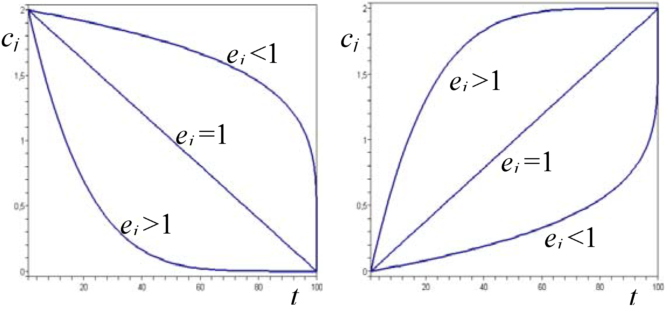
where c_j,t is the value of the coefficient c_j at iteration t, c_j,s at the end of the iterations (t =s) and c_j,0 at the beginning (t=0). The coefficients c_j,0 and c_j,s must be chosen by the user, as well as the power e_j. This last number modulates the variation of the coefficient c_j along the iterations, giving the possibility to the user to increase the rapidity of the variation at the beginning or at the end of the iterations. Some basic examples are shown in Fig. 1: c_j,t increases or decreases quickly at the beginning of the iterations whenever e_j>1, at the end if e_j<1, while the rate of change is constant during iterations if e_j=1.

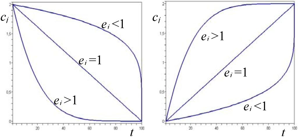
Figure 1. Types of changes of coefficients c_j according to the value of e_j.

Figure 1. Types of changes of coefficients c_j according to the value of e_j.

It is important to notice that the numbers c_j,0, c_j,s and e_j can be chosen independently for j= 0, 1 and 2, letting in this way the user the possibility to increase or decrease, and in different ways, each coefficient c_j independently from the others during iterations. In addition, no restriction are given a priori to the choice of c_j,0 and c_j,s, and they can be negative too.

3.2 Updating the random coefficients r₀, r₁ and r₂

The frequency of updating the random coefficients r₀, r₁ and r₂ can be chosen by the user; in particular, there are three options:

• opt1: r₀, r₁ and r₂ are updated at each iteration (all the particles receive the same value of r₀, r₁ and r₂);
• opt2: r0, r1 and r2 are updated at each particle (all the components of $u_{t+1}^k$ receive the same value of r₀, r₁ and r₂);
• opt3: r₀, r₁ and r₂ are updated at each component of each particle (no repeated values, in principle).

Normally, the third option guarantees a better exploration of the search space, but it is more computing consuming; option 1 is quickest but recommended only for simple problems, as it lowers too much the search capacity of the algorithm, while option 2 is a good compromise for the most part of times.

3.3 Fixing the random coefficient r₀

The random coefficient r₀ can be set equal to 1 for all the iterations; this gives a constant influence of the inertial parameter c₀ for an iteration (and for all the computation if c_0,0=c_0,s). The importance of the inertial parameter has been widely discussed in the literature, see for instance Shi and Eberhart [2]. In the tests performed with ALE-PSO on problems concerning laminates, this choice is not recommended, as it normally diminishes the exploration capability of the algorithm.

3.4 Conservation of the position

Whenever the updated position of a particle gives a higher value of the cost function compared to that of the previous position, ALE-PSO can refuse to update the position, according to a general choice of the user. Actually, this option allows the user to focus the search only on good points and numerical tests revealed that in this way the diagram of convergence of the best individual of each iteration, and mostly that of the population in the average, is regularized and the convergence accelerated. Nevertheless, this option should be activated only for simple problems, as the numerical tests revealed also that this choice increases the probability of convergence towards non global minima.

3.5 Inequality constraints

ALE-PSO can deal also with constrained problems. The strategy for constraint handling in ALE-PSO is essentially a barrier method: the swarm must be feasible at each iteration, i.e. it must be composed by particles respecting all the constraints imposed to the computation. For this reason, the initial swarm is composed by feasible particles and then its updates are guaranteed to be feasible by the following procedure (without lack of generality, we consider here constraints of the form g(x^k)<0):

$$\begin{array}{c}{x}_{t+1}^k=x_t^k+\frac{u_{t+1}^k}{2^{\alpha }},\alpha =0,\hspace{0.17em}1,\hspace{0.17em}2,\mathrm{.....}\\ \text{stop when }g\left(x_{t+1}^k\right)<0.\end{array}$$

(5)

As $x_t^k$ is feasible, this bisection method ensures that, for a sufficiently large α, $x_{t+1}^k$ will be feasible; this procedure is simple, robust and numerical tests have shown that also minima on the boundary of the feasible domain can be reached; it is used also for the control of box constraints. It must be said that ALE-PSO works on a n-dimensional box where all the particles are located at the beginning:

$$a\le x_0^k\le b,$$

(6)

Inequalities (6) being intended to act on each component of the particle x^k. The vectors a and b represent the lower and upper bounds of the particles position in the n-dimensional search space. The above strategy allows respecting conditions (6) at each iteration.

The use of a barrier method is rather important for a PSO, because the evolution of the swarm depends upon two points, p^k and p^g, which must be feasible, but also for the analysis of the convergence of the swarm. In fact, an index of the effectiveness of the algorithm is the control of the average of the objective function over the whole swarm, at each iteration: a good PSO makes all the swarm, and not only the best particle, evolve towards a feasible good point. If the swarm is composed also by unfeasible particles, these can alter significantly the average of the objective, in one sense (decrease) or in the other (increase), which renders difficult to judge about the effectiveness of the algorithm.

3.6 Limitation of the maximum velocity

A classical method to control the stability of the algorithm is the limitation of the maximum velocity to a given value. This is possible also in ALE-PSO; the user defines the maximum allowed velocity component u_max as

$$u_{max}=\nu \hspace{0.17em}\hspace{0.17em}\underset{\hspace{0.17em}i=1,\dots ,n}{\min }\left(b_i-a_i\right),$$

(7)

where $\nu \in [0,1]$ is a reduction coefficient chosen by the user. Nevertheless, this option has proven to be not important in the treatment of laminate design problems with ALE-PSO, because the strategy of control of the box constraints already controls the swarm and at the same time for such problems it is important, at least in the first stage of the calculation, to let the swarm explore as freely as possible the search domain; as limiting the speed contributes to slightly diminish the exploration capability, this option is not recommended for laminates design problems, as it results also in several numerical tests.

4. Trajectory of the numerical parameters

The main problem in the use of a PSO is the tuning of the parameters c₀, c₁, c₂. The stability and convergence of a PSO depends strongly on the choice of these parameters, along with the algorithm's trade off between exploration and exploitation.

As said above, ALE-PSO allows a dynamic tuning of these parameters, i.e. they can vary, according to a power law imposed by the user. So, now the question is: how to establish suitable power laws for the coefficients above? As said in section 2, at the beginning of iterations, c₀ and c₁ should have large values and decrease with iterations, the contrary for c₂. Nevertheless, at each iteration they all should respect some conditions of convergence. Two different set of conditions established by previous researches for the convergence of a standard PSO are considered in this paper, those given by Trelea [5] and those given by Jiang et al [7].

4.1 Trajectory of the parameters in the Trelea's convergence domain

Trelea has considered a simplified case: a deterministic system (i.e. with r₀=1, r₁= r₂=1/2) composed by a single particle. In such a case, he used the theory of dynamical systems to analyse the conditions of convergence of a particle towards an equilibrium point. He has found the following convergence necessary and sufficient conditions:

$$a<1,b>0,2a-b+2>0,$$

(8)

where

$$a=c_0,b=\frac{c_1+c_2}{2}.$$

(9)

These conditions, that determine a triangular domain in the plane (a, b), ensure that the magnitude of the roots of the characteristic equation

$${\lambda }^2-(a-b+1)\lambda +a=0$$

(10)

of the single particle dynamical system is less than one, which is the necessary and sufficient condition for being the equilibrium point an attractor. In addition, the study of the roots of eqn. (10) gives also the quality of the convergence:

• harmonic oscillations around the equilibrium point happen if the roots λ₁ and λ₂ are complex; this happens whenever

  $$a^2+b^2-2ab-2a-2b+1<0;$$

  (11)
• zigzagging around the equilibrium point happens if at least one of the roots (real or complex) has negative real part; this happens whenever

  $$a<0\hspace{1em}\text{or}\hspace{1em}a-b+1<0.$$

  (12)

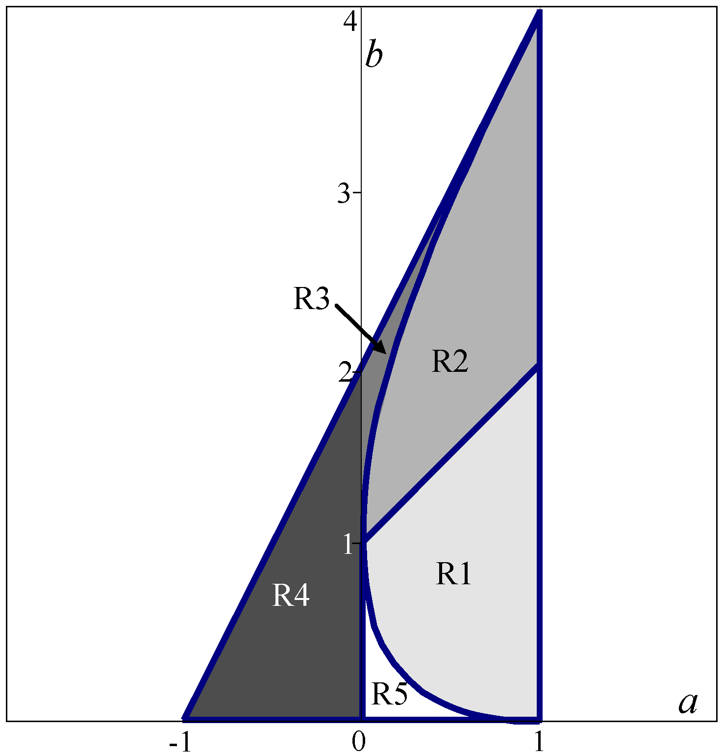
More precisely, we can subdivide the above mentioned triangular domain into five regions (see Fig. 2):

• R1: region where only condition (11) is satisfied (complex roots with positive real parts): oscillatory convergence, with a decay which depends upon the point (a, b);
• R2: region where conditions (11) and (12) are satisfied (complex roots with negative real parts): zigzag superposed to an oscillatory convergence;
• R3: region where only conditions (12) are satisfied and the real roots are both negative: symmetric zigzagging convergence;
• R4: region where only conditions (12) are satisfied and the two real roots have opposite signs: asymmetric zigzagging convergence;
• R5: region where conditions (11) and (12) are not satisfied (two real positive roots): non-oscillatory convergence.

Oscillations and/or zigzagging allows the particle well explore the domain around its equilibrium point, so a choice of the parameters determining a point (a, b) that allows this kind of dynamical behaviour (regions R2 and R3) are well suited for an early stage of the computation; at a final stage, it is better to tend towards conditions allowing quick convergence (i.e., to tend towards regions R4 or R5). So, the update of the parameters should be determined in such a way that their evolution along iterations satisfies this criterion.

Figure 2. Trelea's deterministic convergence domain.

Figure 2. Trelea's deterministic convergence domain.

Actually, each choice of the coefficients c₀, c₁ and c₂ determines a point (a, b) in the convergence region above (or outside it); if the values of c₀, c₁ and c₂ change during iterations, the position of the point (a, b) changes too, describing, with iterations, a trajectory in the plane (a, b). The basic idea is to change the coefficients in order to respect a criterion like the one suggested above (start from region R2 or R3 and evolve towards region R4 or R5) and following a trajectory that belongs to the convergence domain. In this way, convergence conditions are respected at each iteration but the changes of the parameters carries the computation from an initial phase when exploration is preferred to a final phase when exploitation, and the rapidity of the convergence, is preferred. This constitutes a criterion for determining the power laws defining the parameters c₀, c₁ and c₂ update in ALE-PSO.

The analysis of Trelea is simplified and it is based upon a deterministic model; the introduction of the random coefficients r₀, r₁ and r₂ alters the results, and it is questionable if the results found for the deterministic case are still valid. Nevertheless, one could expect that qualitatively things do not change so much, as the same Trelea affirms. The main effect of randomness introduced by coefficients r₀, r₁ and r₂ is an increase of the zigzagging tendency, and hence of exploration, but globally the criterion proposed with the deterministic model can still be considered, if not as a necessary and sufficient condition of convergence, at least as guidelines for the choice of the numerical parameters.

4.2 Trajectory of the parameters in the time domain

Each iteration can be considered as a time step, i.e. t can be identified with time (for this reason vector u is called velocity in the language of PSO's researchers). So, one can consider the changes of the parameters c₀, c₁ and c₂ when they are updated during iterations t; briefly their evolution in the time domain, in the sense specified above, can be considered.

Jiang et al, [7], proposed a different convergence analysis of a PSO standard algorithm: they introduced a stochastic definition of the convergence of the algorithm, in order to take into account the randomness introduced by coefficients r₀, r₁ and r₂. They found the following conditions that can guide the choice of the parameters:

$$0\le a<1,2b>0,0<\phi <{\phi }_1,$$

(13)

where

$$\begin{array}{l}\phi =\left(c_1+c_2\right)\left(1-c_0^2\right)+\frac{1}{6}\left(c_1^2+c_2^2+c_1{c}_2\right)\hspace{0.17em}{c}_0^2-\frac{1}{6}\left(2c_1^2+2c_2^2+3c_1{c}_2\right),\\ {\phi }_1=\frac{1}{6}(1+c_0)\hspace{0.17em}{c}_2^2.\end{array}$$

(14)

Conditions (13) should be respected at each iteration, so they constitute a constraint to the trajectory of the numerical parameters in the time domain. Hence they are conditions that should guide the choice of the power laws determining the update of the numerical parameters in ALE-PSO.

It must be noticed that conditions (13) do not necessarily agree with the Trelea's conditions, as actually they are derived in a different way. For instance, in the Trelea's convergence domain, a negative value of c₀ (=a) is allowed, while it is not admitted by conditions (13). In addition, as the same authors say, conditions (13) are rather difficult to be respected, i.e. they give a small admissible domain for parameters c₀, c₁ and c₂. Nevertheless, conditions (13) constitute some interesting guidelines for the updating of the parameters, and they will be considered in the following.

5. Formulation of optimal design problems for laminates

As said in section 1, the design of laminates must take into account, besides the objective itself (for instance, a sufficient stiffness in one or more directions), also the general elastic properties of the final laminate. The general constitutive law of an elastic laminate is

$$\left\{\begin{array}{c}N\\ M\end{array}\right\}=\left[\begin{array}{cc}A& B\\ B& D\end{array}\right]\left\{\begin{array}{c}{\mathsf{\epsilon }}^o\\ \mathsf{\chi }\end{array}\right\},$$

(15)

where N and M are the tensors of in-plane tractions and of bending moments, ε⁰ is the tensor of in-plane strains for the middle plane, χ is the tensor of curvatures. The fourth order tensors A and D describe respectively the in- and out of-plane behaviour of the plate, while B take into account coupling between them. Usually, designers look for laminates having an orthotropic behaviour, at least in extension, and uncoupled, i.e. B=O, but other elastic properties can also be of interest. All these properties can be taken into account by the following minimization procedure, [13]: consider the quadratic form I(P) of the symmetric matrix H, defined on the 18-dimensional space of the variables P_i:

$$I(P)=P\cdot H\hspace{0.17em}P=H_{ij}{P}_i{P}_j,i,j=1,\dots ,18$$

(16)

with the components of vector P given by

$$\begin{array}{l}{P}_1=\frac{{\overline{T}}_0}{h\hspace{0.17em}M},\hspace{0.17em}\hspace{0.17em}{P}_2=\frac{{\overline{T}}_1}{h\hspace{0.17em}M},\hspace{0.17em}\hspace{0.17em}{P}_3=\frac{{\overline{R}}_0}{h\hspace{0.17em}M},\hspace{0.17em}\hspace{0.17em}{P}_4=\frac{{\overline{R}}_1}{h\hspace{0.17em}M},\hspace{0.17em}\hspace{0.17em}{P}_5={\overline{\Phi }}_0,\hspace{0.17em}\hspace{0.17em}{P}_6={\overline{\Phi }}_1,\\ P_7=\frac{2\hspace{0.17em}{\widehat{T}}_0}{h^2\hspace{0.17em}M},\hspace{0.17em}\hspace{0.17em}{P}_8=\frac{2\hspace{0.17em}{\widehat{T}}_1}{h^2\hspace{0.17em}M},\hspace{0.17em}\hspace{0.17em}{P}_9=\frac{2\hspace{0.17em}{\widehat{R}}_0}{h^2\hspace{0.17em}M},\hspace{0.17em}\hspace{0.17em}{P}_{10}=\frac{2\hspace{0.17em}{\widehat{R}}_1}{h^2\hspace{0.17em}M},\hspace{0.17em}\hspace{0.17em}{P}_{11}={\widehat{\Phi }}_0,\hspace{0.17em}\hspace{0.17em}{P}_{12}={\widehat{\Phi }}_1,\\ P_{13}=\frac{12\hspace{0.17em}{\tilde{T}}_0}{h^3\hspace{0.17em}M},\hspace{0.17em}\hspace{0.17em}{P}_{14}=\frac{12\hspace{0.17em}{\tilde{T}}_1}{h^3\hspace{0.17em}M},\hspace{0.17em}\hspace{0.17em}{P}_{15}=\frac{12\hspace{0.17em}{\tilde{R}}_0}{h^3\hspace{0.17em}M},\hspace{0.17em}\hspace{0.17em}{P}_{16}=\frac{12\hspace{0.17em}{\tilde{R}}_1}{h^3\hspace{0.17em}M},\hspace{0.17em}\hspace{0.17em}{P}_{17}={\tilde{\Phi }}_0,\hspace{0.17em}\hspace{0.17em}{P}_{18}={\tilde{\Phi }}_1.\end{array}$$

(17)

Here, h is the total laminate thickness while M is a factor, whose dimensions are those of an elastic modulus, used to obtain non-dimensional variables, that can be chosen in various ways. In addition,

$$\begin{array}{l}{\overline{T}}_0,{\widehat{T}}_0,{\tilde{T}}_0=\frac{1}{\mu }{\displaystyle \sum _{k=1}^{np}{T}_{0_k}(z_k^{\mu }-z_{k-1}^{\mu })}\text{ ,}\\ {\overline{T}}_1,{\widehat{T}}_1,{\tilde{T}}_1=\frac{1}{\mu }{\displaystyle \sum _{k=1}^{np}{T}_{1_k}(z_k^{\mu }-z_{k-1}^{\mu })},\\ {\overline{R}}_0{e}^{4i{\overline{\Phi }}_0},{\widehat{R}}_0{e}^{4i{\widehat{\Phi }}_0},{\tilde{R}}_0{e}^{4i{\tilde{\Phi }}_0}=\frac{1}{\mu }{\displaystyle \sum _{k=1}^{np}{R}_{0_k}{e}^{4i({\Phi }_{0_k}+{\delta }_k)}(z_k^{\mu }-z_{k-1}^{\mu })},\\ {\overline{R}}_1{e}^{4i{\overline{\Phi }}_1},{\widehat{R}}_1{e}^{4i{\widehat{\Phi }}_1},{\tilde{R}}_1{e}^{4i{\tilde{\Phi }}_1}=\frac{1}{\mu }{\displaystyle \sum _{k=1}^{np}{R}_{1_k}{e}^{4i({\Phi }_{1_k}+{\delta }_k)}(z_k^{\mu }-z_{k-1}^{\mu })},\end{array}$$

(18)

are, in complex form, the 18 polar components of, respectively, tensor A, B and D, with μ=1 for A, μ=2 for B and μ=3 for D; np is the number of plies in the stack and δ_k is the orientation angle of the k-th ply; T_0k, T_1k, R_0k, R_1k, Φ_0k and Φ_1k are the polar parameters of the k-th layer. The polar parameters of an elastic plane tensor L are given, in complex form, by the following functions of the Cartesian components of L:

$$\begin{array}{rrrrrrr}\hfill 8T_0& \hfill =& \hfill L_{1111}& \hfill -2L_{1122}& \hfill +4L_{1212}& \hfill +L_{2222},& \\ \hfill 8T_1& \hfill =& \hfill L_{1111}& \hfill +2L_{1122}& & \hfill +L_{2222},& \\ \hfill 8R_0{\text{ e}}^{\text{4}i{\Phi }_{\text{0}}}& \hfill =& \hfill L_{1111}& \hfill -2L_{1122}& \hfill -4L_{1212}& \hfill +L_{2222}& \hfill +4i\left(L_{1112}-L_{2212}\right),\\ \hfill 8R_1{\text{ e}}^{\text{2}i{\Phi }_{\text{1}}}& \hfill =& \hfill L_{1111}& & & \hfill -L_{2222}& \hfill +2i\left(L_{1112}+L_{2212}\right).\end{array}$$

(19)

The advantage of using polar parameters is their capability to express as simply as possible the symmetries of the elastic behaviour; actually,

• L is orthotropic if and only if

  $${\Phi }_0-{\Phi }_1=K\frac{\pi }{4},K=0,\hspace{0.17em}1;$$

  (20)
• L is R₀-orthotropic, (Vannucci, [16]), if and only if

  $$R_0=0.$$

  (21)
• L is square-symmetric (that is, its components are invariant under rotations of π/4) if and only if

  $$R_1=0;$$

  (22)
• L is isotropic if and only if

  $$R_0=R_1=0.$$

  (23)

For more details on the results of the polar method, the reader is addressed to the original paper of Verchery, [14], or to [17].

H is a symmetric matrix of real coefficients: the choice of its components H_ij determines the kind of problem to be treated. Several choices are possible, so several different problems can be stated in the same way, simply changing the H_ij. H is positive semi-definite and each problem of determining a laminate having some specified general elastic properties can be stated as follows: find an absolute minimum of (16) for a given H. As H is positive semi-definite, these minimums are zero-valued (except in the case of k=1 orthotropy). Clearly, to solve such a problem means to find a vector P satisfying the above statement. As P=P(δ_k), cfr. eqns. (17) and (18), the true design variables of the problem are the orientations δ_k. Eqns. (18) are highly non-linear and non convex with respect to the δ_k, so also function (16) is non-linear and non-convex.

Finally, a unique mathematical form has been given to several different problems of laminate design: the search for the minimum of a positive semi-definite form, which is a classical problem of structural non-convex optimisation. It is worth noting that parameters P_i generalise the concept of lamination parameters introduced by Miki, [18,19], and successively widely used by several authors, but unlike these they have some advantages: they are based upon tensor invariants linked to elastic symmetries, so their use allows a very simple statement of problems concerning these symmetries and in addition they make directly appear the orientation of the reference or material frame.

Of course, the optimal design of laminates cannot be reduced to the unique design of elastic properties; normally, designers want to minimize or maximize a given quantity (volume, stiffness etc.) or to obtain minimum requirements. For the sake of shortness, we consider in the following only this last kind of problems, which can be formalised, in a general way, as:

$$\begin{array}{l}\underset{{\delta }_k,\hspace{0.17em}k=1,\dots ,np}{\text{min}}I\left[P\left({\delta }_k\right)\right],\\ \text{with}\hspace{1em}{g}_j\left[P\left({\delta }_k\right)\right]\le 0,j=1,\mathrm{..},nc,\end{array}$$

(24)

with $g_j\left[P\left({\delta }_k\right)\right]$ a generic constraint imposed to the problem and nc the total number of constraints. In the next section, some numerical examples of this type solved with ALE-PSO are presented.

6. Numerical examples

Several examples concerning different problems of laminates design have been treated with ALE-PSO, the results concerning some of them are presented below. The objective of this paper is the adaptive tuning of numerical parameters, so some characteristics of the computations have been conserved through all the runs of the code, in order to assess the importance of adaptive tuning only. In particular:

• the population size is constant, m=100;
• the number of generations has been fixed to s=300;
• the original population has been sorted randomly once and for all for all the tests, i.e. the tests have been performed on the same starting population for all the cases;
• the option opt3 has been chosen for the updating of the random coefficients, cfr. § 3.2, also for r₀ (it is not fixed to 1);
• there is no limit on the highest velocity, but the position of a particle is controlled to remain in the domain [−90°, 90°]ⁿ (the design variables are the orientation angles of the layers).

Five different types of calculations have been made, the first two with constant parameters c₀, c₁, c₂, whose values have been suggested by Clerc and Kennedy [4], test T1, and by Trelea [5], test T2. The three others tests have been done with a trajectory of adaptive parameters; the data for the parameters are summarized in Tab. 1. In addition, the variations and trajectories of the tests T3, T4 and T5 are presented in Fig. 3 and Fig. 4. Tests T1 and T2 reduces to points in the Trelea's domain, and in horizontal lines (not traced in Fig. 3) in the time domain. It can be noticed that only the test T5 respects both the conditions by Trelea and by Jiang et al. (for test T1, φ = −0.384, while for test T2 φ = −0.328). Actually, it is very difficult to respect all the conditions proposed by Jiang et al, especially the condition φ>0; in fact, to respect this condition it is important to use low values for c₀, but this limits, especially in the first part of the calculation, the exploration of the domain, as it results from a long series of numerical tests.

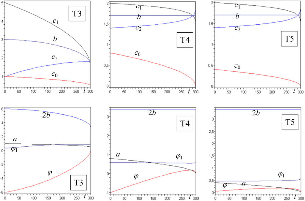
Figure 3. Time-domain trajectories of parameters c₀(=a), c₁, c₂, b, φ and φ₁ for the tests T3, T4 and T5.

Figure 3. Time-domain trajectories of parameters c₀(=a), c₁, c₂, b, φ and φ₁ for the tests T3, T4 and T5.

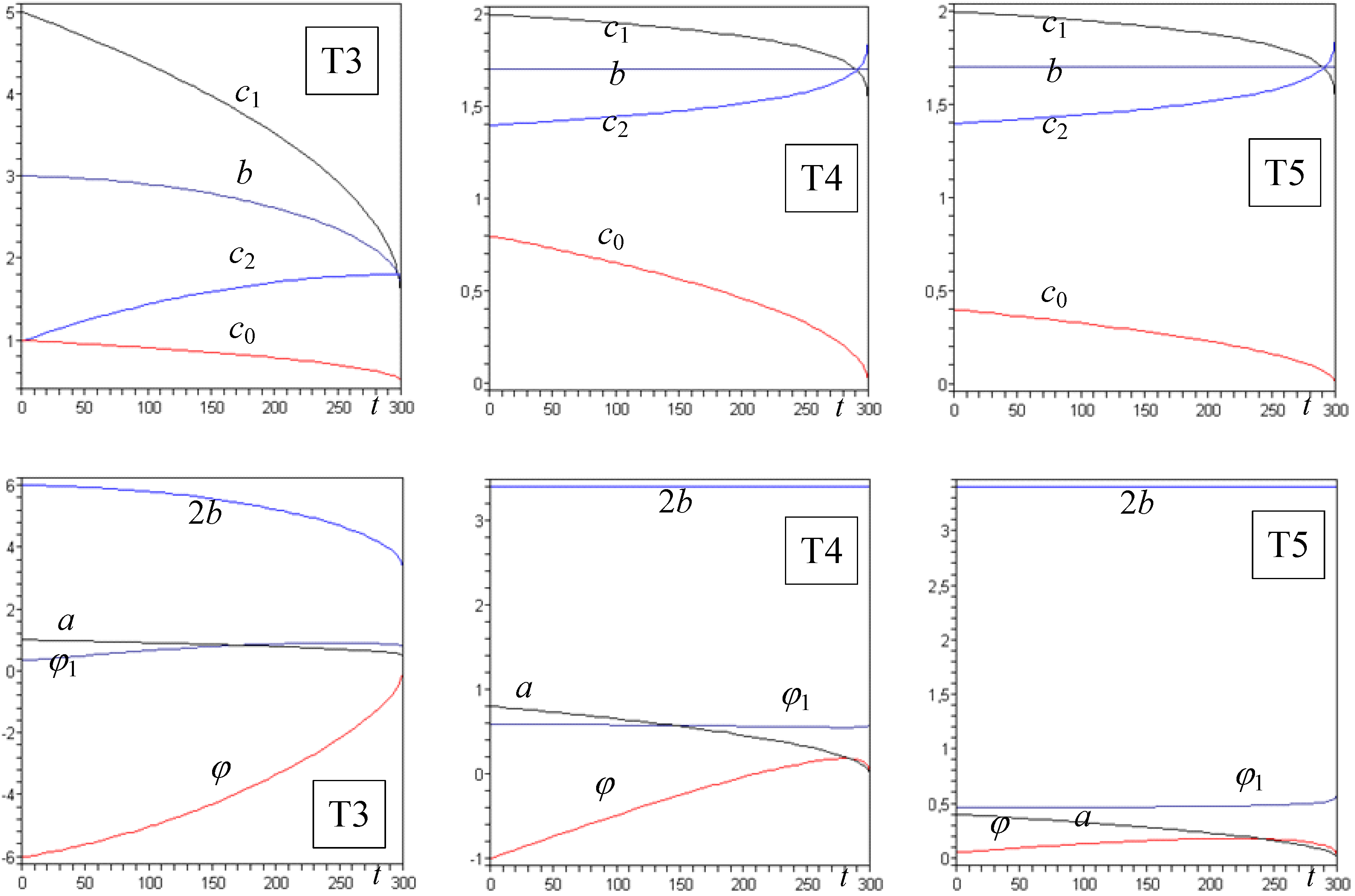
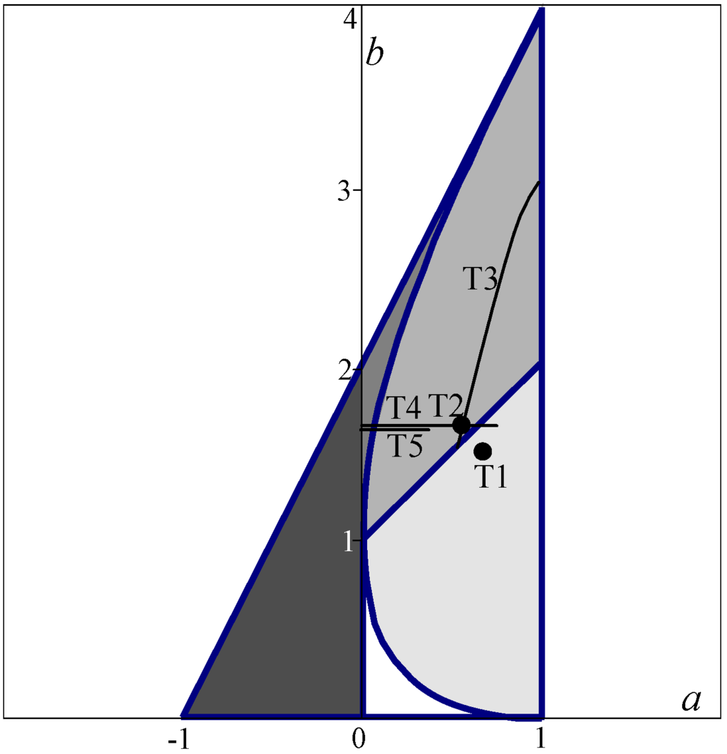
Figure 4. Trajectories in the Trelea's convergence domain of tests T1 to T5.

Figure 4. Trajectories in the Trelea's convergence domain of tests T1 to T5.

Table 1. Numerical data for the tuning of parameters c₀, c₁, c₂ in the tests.

Test	c0,0	c0,s	e0	c1,0	c1,s	e1	c2,0	c2,s	e2
T1	0.729	0.729	0	1.490	1.490	0	1.490	1.490	0
T2	0.600	0.600	0	1.700	1.700	0	1.700	1.700	0
T3	1.000	0.500	0.5	5.000	1.500	0.5	1.000	1.800	2
T4	0.800	0.000	0.5	2.000	1.400	0.2	1.400	2.000	0.2
T5	0.400	0.000	0.5	2.000	1.400	0.2	1.400	2.000	0.2

Table 1. Numerical data for the tuning of parameters c₀, c₁, c₂ in the tests.

Test	c0,0	c0,s	e0	c1,0	c1,s	e1	c2,0	c2,s	e2
T1	0.729	0.729	0	1.490	1.490	0	1.490	1.490	0
T2	0.600	0.600	0	1.700	1.700	0	1.700	1.700	0
T3	1.000	0.500	0.5	5.000	1.500	0.5	1.000	1.800	2
T4	0.800	0.000	0.5	2.000	1.400	0.2	1.400	2.000	0.2
T5	0.400	0.000	0.5	2.000	1.400	0.2	1.400	2.000	0.2

In addition, all the examples refer to laminates composed by identical T300-5208 carbon-epoxy plies, with a thickness of 0.125 mm and whose characteristics are given in Tab. 2, [20]. In the following, the numerical results of three examples are shown; each test has been run 100 times, and the statistics of the runs are given (mean and standard deviation). In Appendix, the results obtained with the above trajectories of the parameters and concerning a well known benchmark are also shown.

Table 2. Technical, Cartesian and polar constants of carbon-epoxy T300-5208 plies (GPa).

E1	E2	G12	ν12	Q11	Q22	Q66	Q12	T0	T1	R0	R1	Φ0	Φ1
181.00	10.30	7.17	0.28	18 1.81	10.35	7.17	2.89	26.88	24.74	19.71	21.43	0°	0°

Table 2. Technical, Cartesian and polar constants of carbon-epoxy T300-5208 plies (GPa).

E1	E2	G12	ν12	Q11	Q22	Q66	Q12	T0	T1	R0	R1	Φ0	Φ1
181.00	10.30	7.17	0.28	18 1.81	10.35	7.17	2.89	26.88	24.74	19.71	21.43	0°	0°

6.1 Example 1

This is the case of the search of fully isotropic laminates with twelve plies. It is a very difficult problem in laminate designs, already treated in the past by the author and co-workers, [21], and by other researchers, [22]; actually, it seems, up to now, that it is impossible to obtain a fully isotropic laminate composed by less than 12 identical plies; this example is a sort of benchmark in the laminates design field.

The case of fully isotropy, that comprehends also bending-extension uncoupling, is determined by the choice $H_{ii}=1,\hspace{0.17em}\hspace{0.17em}i=3,\hspace{0.17em}4,\hspace{0.17em}9,\hspace{0.17em}10,\hspace{0.17em}15\text{,}\hspace{0.17em}16,$ the other components being null, so that function I(P) reduces to

$$I(P)=P_3^2+P_4^2+P_9^2+P_{10}^2+P_{15}^2+P_{16}^2=0.$$

(25)

Quantities P_i must be computed through eq. (18), the problem is hence strongly non-convex, the design variables being the angles δ_k.

The results of the numerical tests are summarised in Tab. 3. For each tests, composed, as already said, by 100 runs of ALE-PSO with the same initial swarm, two quantities, obtained in a run for the objective function, are considered: the best value of the average on the swarm and the value of the best particle in the swarm (i.e. the particle having the lowest value of the objective function). For both these quantities, the statistics data relative to all the 100 runs, are: the mean value, the standard deviation, the best value, the worst value and the number of evaluations n_eval of the objective function to obtain the quantity's mean value.

Of course, the exact solution being valued 0, the data reported in columns 3, 5 and 6 of Tab. 3 are to be considered as numerical residual of the computation. Under a mechanical point of view, a residual of the magnitude 10⁻² for this problem can be considered as technically acceptable, i.e. the final laminate with a value of I(P)~10⁻² can be considered very close to be fully isotropic, under a practical point of view. In Fig. 5, for instance, the case of a laminate with I(P)= 0.023 is shown; it corresponds to the best particle in test T3, whose stacking sequence is [−16.43°, −70.38°, 66.70°, 31.97°, 31.76°, −59.02°, 78.65°, −12.13°, −12.34°, −47.06°, −90.00°, 36.06°]. The directional diagrams of the normalised Cartesian components A_xx*= A_xx/h, B_xx*=2 B_xx/h² and D_xx*=12 D_xx/h³ are shown; actually, B_xx*~0 (almost a dot in the centre of the plot), which confirms that the laminate is uncoupled, while A_xx*~D_xx* and they describe a curve very close to a circle of radius T₀+2T₁=76.36 GPa, as it must be for isotropy.

Table 3. Results of the tests T1 to T5 for example 1.

Test	Run’s best	Mean value	Standard deviation	Best value	Worst value	neval
T1	average	0.203	0.194	0.091	0.686	23830
	particle	0.104	0.077	0.023	0.310	29860
T2	average	0.209	0.185	0.024	0.569	27110
	particle	0.114	0.081	0.023	0.310	29980
T3	average	0.211	0.028	0.023	0.860	27030
	particle	0.061	0.022	0.023	0.090	30000
T4	average	0.102	0.072	0.034	0.243	29900
	particle	0.075	0.023	0.034	0.097	29940
T5	average	0.186	0.225	0.024	0.800	29140
	particle	0.126	0.097	0.024	0.383	29980

Table 3. Results of the tests T1 to T5 for example 1.

Test	Run’s best	Mean value	Standard deviation	Best value	Worst value	neval
T1	average	0.203	0.194	0.091	0.686	23830
	particle	0.104	0.077	0.023	0.310	29860
T2	average	0.209	0.185	0.024	0.569	27110
	particle	0.114	0.081	0.023	0.310	29980
T3	average	0.211	0.028	0.023	0.860	27030
	particle	0.061	0.022	0.023	0.090	30000
T4	average	0.102	0.072	0.034	0.243	29900
	particle	0.075	0.023	0.034	0.097	29940
T5	average	0.186	0.225	0.024	0.800	29140
	particle	0.126	0.097	0.024	0.383	29980

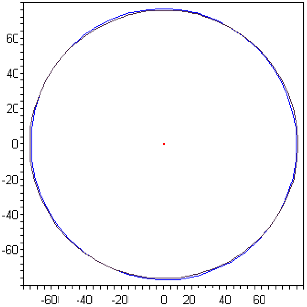
Figure 5. Directional diagrams of A_xx*, D_xx*, almost superposed, and B_xx*, reduced to a dot in the centre (GPa).

Figure 5. Directional diagrams of A_xx*, D_xx*, almost superposed, and B_xx*, reduced to a dot in the centre (GPa).

6.2 Example 2

This is the case of a rectangular laminated plate with 12 plies, designed to be uncoupled and orthotropic in bending, with axes of orthotropy at 0° and 90°; the plate is simply supported, with side lengths along the axes x and y respectively equal to a and b. The additional requirement is that the frequency of the first mode of the bending vibrations must be greater than a minimum specified value ω₀. So, the objective function is still I(P), but now $H_{ii}=1,\hspace{0.17em}\hspace{0.17em}i=\hspace{0.17em}9,\hspace{0.17em}10,\hspace{0.17em}17\text{,}\hspace{0.17em}18,$ so that

$$I(P)=P_9^2+P_{10}^2+P_{17}^2+P_{18}^2=0,$$

(26)

and the problem is constrained by the condition

$$g(P)={\omega }_0-{\omega }_{pq}(P)\le 0$$

(27)

where the frequency ω_pq(P) of the mode having p and q half waves respectively along x and y, is given by, see [23],

$${\omega }_{pq}^2=\frac{{\pi }^4{p}^4{h}^3}{12\sigma \hspace{0.17em}{a}^4}\sqrt{R_0^2+R_1^2}{(1+{\chi }^2)}^2\phi ({\xi }_0,{\xi }_1)\hspace{0.17em},$$

(28)

with

$$\phi ({\xi }_0,{\xi }_1)=\tau +\frac{1}{\sqrt{1+{\rho }^2}}\left[{(-1)}^K\rho {\xi }_0\frac{{\chi }^4-6{\chi }^2+1}{{(1+{\chi }^2)}^2}+4{\xi }_1\frac{1-{\chi }^2}{1+{\chi }^2}\right].$$

(30)

h is the total thickness of the plate, σ its mass per unit area and the three dimensionless quantities χ, ρ and τ, represent respectively the geometric/modal, anisotropic and isotropic parts of the problem:

$$\chi =\frac{qa}{pb},\rho =\frac{R_0}{R_1},\tau =\frac{T_0+2T_1}{\sqrt{R_0^2+R_1^2}}.$$

(31)

Moreover,

$${\xi }_0=\frac{1}{n{p}^3}{\displaystyle {\sum }_{j=1}^{np}{d}_j\cos 4{\delta }_j,}\hspace{1em}{\xi }_1=\frac{1}{n{p}^3}{\displaystyle {\sum }_{j=1}^{np}{d}_j\cos 2{\delta }_j,}$$

(32)

are the classical bending lamination parameters, the coefficients d_j being

$$d_j=12j(j-np-1)+4+3np(np+2).$$

(33)

The results of the numerical tests for this example are shown in Table 4; they refer to the case of a plate with sides a=1 m, b=0.5 m, designed to have ω₁₁≥ ω₀= 150 s⁻¹; the mass of the plate per unit of area is σ =2.4 kg/m² (12 plies of carbon-epoxy T300-5208). The best result is obtained with the trajectory T3: [−66.15°, 66.53°, 44.83°, −36.44°, 48.52°, −5.68°, 77.57°, −89.94°, −84.48°, 38.45°, 57.48°, −46.03°]. For this sequence, the objective function is very close to zero (7.20×10⁻³⁵) and the frequency ω₁₁=162.72 s⁻¹. The elastic properties of this laminate are shown in Table 5 and in Fig. 6; they show that the laminate is really uncoupled (all the polar components of B are practically null) and K=1 orthotropic in bending, with orthotropy axes at 0° and 90° (Φ₀=45°, Φ₁=90°); in addition, the extension behaviour is completely anisotropic, as a result of the fact that no requirement on A has been formulated.

It is worth to recall that bending orthotropy together with uncoupling is a hard requirement to be obtained, cfr. [24]; this example shows that ALE-PSO can easily find uncoupled laminates that are orthotropic in bending.

Table 4. Results of the tests T1 to T5 for example 2.

Test	Run’s best	Mean value	Standard deviation	Best value	Worst value	neval
T1	average	9.78×10−3	4.69×10−3	4.50×10−3	1.80×10−2	25510
	particle	1.04×10−18	1.25×10−18	8.00×10−21	3.30×10−18	29800
T2	average	1.37×10−2	8.14×10−3	4.50×10−3	3.20×10−2	26540
	particle	1.47×10−18	3.32×10−18	8.80×10−29	9.90×10−18	29760
T3	average	1.14×10−2	4.58×10−2	4.50×10−2	2.10×10−2	26040
	particle	1.83×10−31	4.74×10−31	7.20×10−35	1.50×10−30	29670
T4	average	1.18×10−2	5.24×10−3	6.60×10−3	2.20×10−2	25840
	particle	3.00×10−9	9.49×10−9	1.30×10−34	3.00×10−8	27800
T5	average	9.33×10−3	3.97×10−3	1.20×10−3	1.30×10−2	24640
	particle	2.24×10−18	6.60×10−18	5.70×10−34	2.10×10−17	27990

Table 4. Results of the tests T1 to T5 for example 2.

Test	Run’s best	Mean value	Standard deviation	Best value	Worst value	neval
T1	average	9.78×10−3	4.69×10−3	4.50×10−3	1.80×10−2	25510
	particle	1.04×10−18	1.25×10−18	8.00×10−21	3.30×10−18	29800
T2	average	1.37×10−2	8.14×10−3	4.50×10−3	3.20×10−2	26540
	particle	1.47×10−18	3.32×10−18	8.80×10−29	9.90×10−18	29760
T3	average	1.14×10−2	4.58×10−2	4.50×10−2	2.10×10−2	26040
	particle	1.83×10−31	4.74×10−31	7.20×10−35	1.50×10−30	29670
T4	average	1.18×10−2	5.24×10−3	6.60×10−3	2.20×10−2	25840
	particle	3.00×10−9	9.49×10−9	1.30×10−34	3.00×10−8	27800
T5	average	9.33×10−3	3.97×10−3	1.20×10−3	1.30×10−2	24640
	particle	2.24×10−18	6.60×10−18	5.70×10−34	2.10×10−17	27990

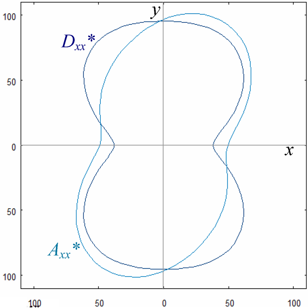
Figure 6. Directional diagrams of A_xx* and D_xx* (B_xx*~ 0) for example 2 (GPa).

Figure 6. Directional diagrams of A_xx* and D_xx* (B_xx*~ 0) for example 2 (GPa).

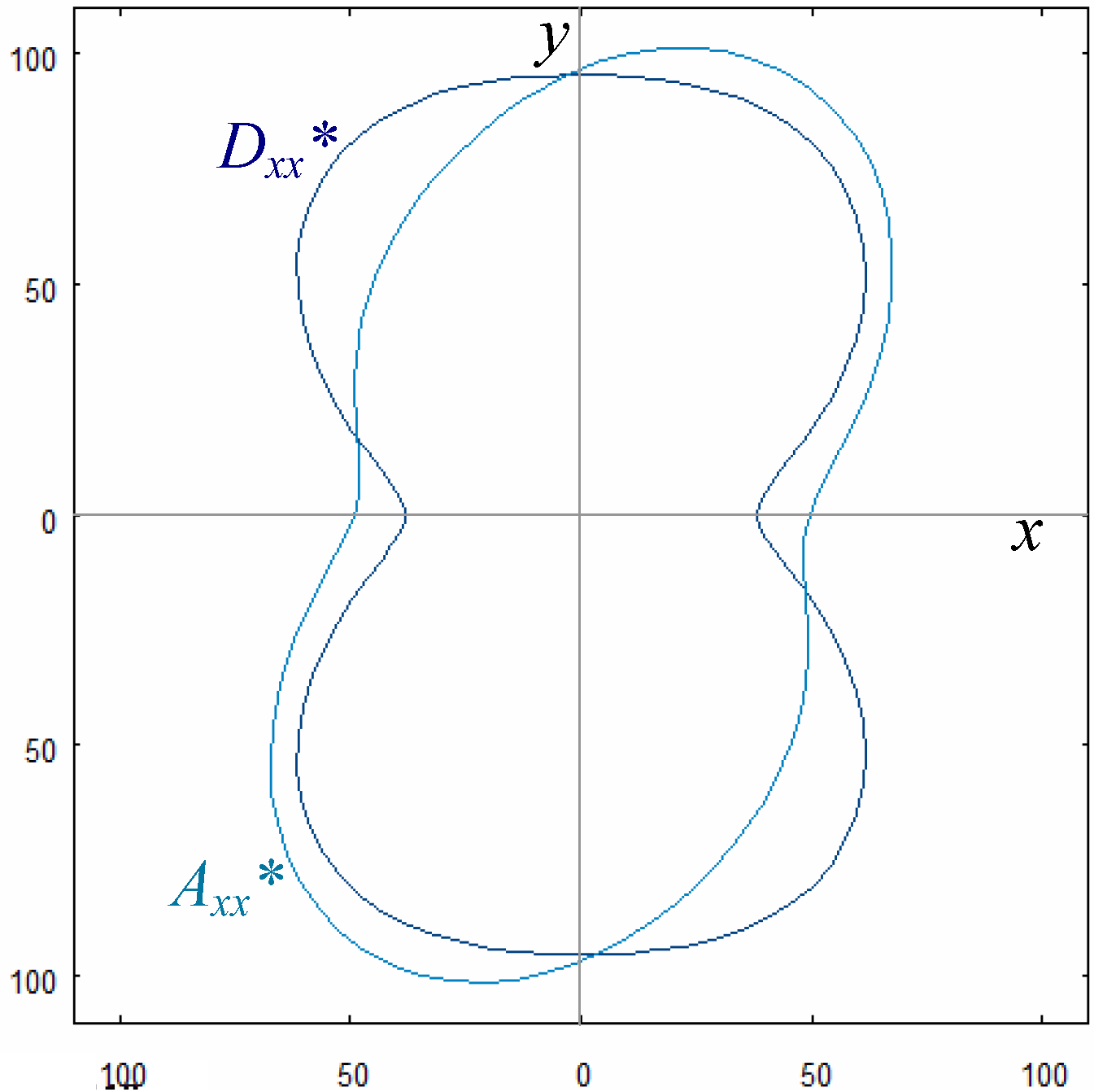
Table 5. Example 2: technical, Cartesian and polar constants of the best solution laminate; C_ij is a generic Cartesian component (GPa).

	Ex	Ey	Gxy	νxy	Cxx	Cyy	Css	Cxy	Cxs	Cys
A*	42.39	81.15	29.11	0.26	49.38	96.79	30.17	25.89	3.94	9.91
B*	-	-	-	-	−7.3×10−4	−8.5×10−4	4.6×10−3	4.6×10−3	3.8×10−3	−1.2×10−2
D*	27.38	68.38	36.42	0.34	38.21	95.43	36.43	32.15	0	0

	Ex	Ey	Gxy	νxy	Cxx	Cyy	Css	Cxy	Cxs	Cys
A*	42.39	81.15	29.11	0.26	49.38	96.79	30.17	25.89	3.94	9.91
B*	-	-	-	-	−7.3×10−4	−8.5×10−4	4.6×10−3	4.6×10−3	3.8×10−3	−1.2×10−2
D*	27.38	68.38	36.42	0.34	38.21	95.43	36.43	32.15	0	0

	T0	T1	R0	R1	Φ0	Φ1
A*	26.88	24.74	4.44	6.86	−34.43°	74.85°
B*	0	0	9.3×10−6	2.3×10−6	-	-
D*	26.88	24.74	9.55	7.15	45°	90°

	T0	T1	R0	R1	Φ0	Φ1
A*	26.88	24.74	4.44	6.86	−34.43°	74.85°
B*	0	0	9.3×10−6	2.3×10−6	-	-
D*	26.88	24.74	9.55	7.15	45°	90°

6.3 Example 3

This is the case of a 8-ply laminate designed to be orthotropic in bending, uncoupled and with the Young’s modulus in the directions x and y constrained to satisfy respectively the conditions E_x ≥E₁=90 GPa and E_y ≥E₂=90 GPa. In addition, it is required that the orientation angles take values each 5°, i.e. 0°, 5°, 10° and so on. The objective function is the same of example 2, but now the constraints to be satisfied are, see [25],

$$\begin{array}{c}{E}_x=\frac{8[T_0{T}_1+{(-1)}^K{T}_1{R}_0{\xi }_0-2R_1^2{\xi }_1^2]}{T_0+2T_1+{(-1)}^K{R}_0{\xi }_0-4R_1{\xi }_1}\ge E_1,\\ E_y=\frac{8[T_0{T}_1+{(-1)}^K{T}_1{R}_0{\xi }_0-2R_1^2{\xi }_1^2]}{T_0+2T_1+{(-1)}^K{R}_0{\xi }_0+4R_1{\xi }_1}\ge E_2.\end{array}$$

(34)

Table 6. Results of the tests T1 to T5 for example 3.

Test	Run’s best	Mean value	Standard deviation	Best value	Worst value	neval
T1	average	8.30×10−3	2.38×10−3	4.80×10−3	1.30×10−2	25140
	particle	6.25×10−4	9.45×10−5	5.70×10−6	2.40×10−4	9510
T2	average	1.66×10−2	1.25×10−2	1.70×10−3	3.70×10−2	25010
	particle	8.91×10−4	1.35×10−3	2.20×10−6	3.70×10−3	3320
T3	average	8.88×10−3	3.63×10−3	4.30×10−3	1.50×10−2	25480
	particle	7.11×10−4	1.19×10−4	1.00×10−6	3.40×10−4	4910
T4	average	3.59×10−3	5.31×10−3	2.50×10−6	1.80×10−2	22150
	particle	8.32×10−4	8.34×10−4	2.50×10−6	2.50×10−3	5710
T5	average	1.23×10−3	1.88×10−3	1.10×10−4	6.40×10−3	21400
	particle	4.55×10−4	5.65×10−4	8.50×10−5	2.00×10−3	2980

Table 6. Results of the tests T1 to T5 for example 3.

Test	Run’s best	Mean value	Standard deviation	Best value	Worst value	neval
T1	average	8.30×10−3	2.38×10−3	4.80×10−3	1.30×10−2	25140
	particle	6.25×10−4	9.45×10−5	5.70×10−6	2.40×10−4	9510
T2	average	1.66×10−2	1.25×10−2	1.70×10−3	3.70×10−2	25010
	particle	8.91×10−4	1.35×10−3	2.20×10−6	3.70×10−3	3320
T3	average	8.88×10−3	3.63×10−3	4.30×10−3	1.50×10−2	25480
	particle	7.11×10−4	1.19×10−4	1.00×10−6	3.40×10−4	4910
T4	average	3.59×10−3	5.31×10−3	2.50×10−6	1.80×10−2	22150
	particle	8.32×10−4	8.34×10−4	2.50×10−6	2.50×10−3	5710
T5	average	1.23×10−3	1.88×10−3	1.10×10−4	6.40×10−3	21400
	particle	4.55×10−4	5.65×10−4	8.50×10−5	2.00×10−3	2980

The results of the tests made for this example are shown in Tab. 6. The best result is once again found by trajectory T3, to which corresponds the anti-symmetric sequence [−5°, −85°, 45°, −55°, 55°, −45°, 85°, 5°]; for this laminate, the value of the objective function is 10⁻⁶, E_x= 112.31 GPa and E_y=66.21 GPa. The elastic properties of this laminate are shown in Table 6 and in Fig. 7; the same remarks made on example 2 can be done again, but now the value of the components of B* are larger, as a consequence of the fact that orientations are not continuous variables and that the layers number is smaller. Nevertheless, when compared with the corresponding components of A* and D*, they are still negligible, i.e. the solution is technically acceptable. In addition, now A* and D* are both K=0 orthotropic, consequence of the anti-symmetry of the stack.

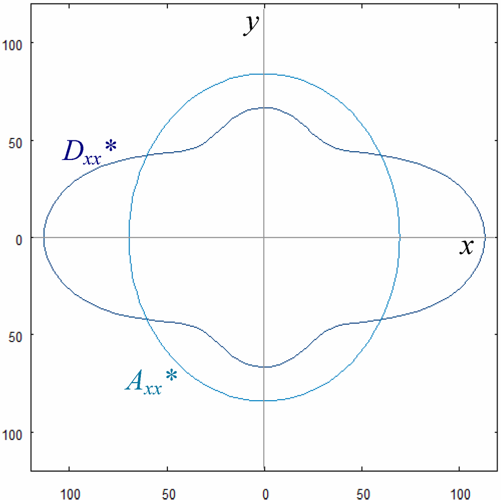
Figure 7. Directional diagrams of A_xx* and D_xx* (B_xx*~ 0) for example 3 (GPa).

Figure 7. Directional diagrams of A_xx* and D_xx* (B_xx*~ 0) for example 3 (GPa).

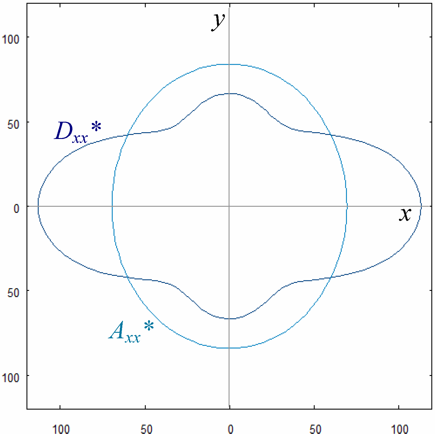
Table 6. Example 3: technical, Cartesian and polar constants of the best solution laminate; C_ij is a generic Cartesian component (GPa).

	Ex	Ey	Gxy	νxy	Cxx	Cyy	Css	Cxy	Cxs	Cys
A*	63.82	77.27	26.32	0.26	69.60	84.26	26.32	22.05	0	0
B*	-	-	-	-	0	0	0	0	0.056	0.006
D*	112.31	66.21	13.06	0.13	113.47	66.89	13.06	8.79	0	0

	Ex	Ey	Gxy	νxy	Cxx	Cyy	Css	Cxy	Cxs	Cys
A*	63.82	77.27	26.32	0.26	69.60	84.26	26.32	22.05	0	0
B*	-	-	-	-	0	0	0	0	0.056	0.006
D*	112.31	66.21	13.06	0.13	113.47	66.89	13.06	8.79	0	0

	T0	T1	R0	R1	Φ0	Φ1
A*	26.88	24.74	0.56	1.83	0°	90°
B*	0	0	0.025	0.016	22.5°	45°
D*	26.88	24.74	13.81	5.82	0°	0°

	T0	T1	R0	R1	Φ0	Φ1
A*	26.88	24.74	0.56	1.83	0°	90°
B*	0	0	0.025	0.016	22.5°	45°
D*	26.88	24.74	13.81	5.82	0°	0°

7. Comments and conclusions

Some considerations can be done about the results shown above. First of all, they all are some rather exigent problems in laminate design, and ALE-PSO has been able to find numerical solutions that are very close to an exact one. A second remark concerns the difference in the order of magnitude of the residuals: it is very small in example 2, while it increases in example 3 and even more in example 1. This is intrinsic to the problem: whilst the case treated in example 2 uses continuous variables and has 12 plies, so that solutions with a residual extremely close to zero can be found, in example 3 there are discrete variables and only 8 layers. These two circumstances contribute to render much more intricate the problem; in fact, it is well known that the difficulty in satisfying the condition of B null increases when the number of plies decreases, and in addition the requirement that the plies can take only discrete values diminishes the number of solutions. For example 1, as already said, the objective is so difficult that it is taken as a sort of benchmark in problems of laminate design. Nevertheless, several solutions have been found, in a very short computing time: all the examples run for no more than 3.5 seconds on a common laptop (the author and co-workers had used in the past a genetic algorithm to treat analogous problems, and example 1 was solved using a population of 2000 individuals and 3000 iterations, for a time of about 30 minutes to be solved with the same order of magnitude of the residual; the best solution found by ALE-PSO has used a population of 100 particles and 300 iterations, i.e. 200 times less evaluations of the objective function; for more details on the use of genetic algorithms in the global design of laminates, see [15], [21].

More interesting is to compare the trajectories of the parameters to determine the most performing one. To this purpose it is worth to consider the cases of the expected and best value of the residual, for the swarm average and best particle; this is done in Tab. 7, where the trajectory giving the best result for each quantity is indicated, using the results of Tab. 3, Tab. 4 and Tab. 6.

Table 7. Summary of the best trajectories for each case.

Example	Expected value		Best value
	average	particle	average	particle
1	T4	T3	T3	T3
2	T5	T3	T5	T3
3	T5	T5	T4	T3

Table 7. Summary of the best trajectories for each case.

Example	Expected value		Best value
	average	particle	average	particle
1	T4	T3	T3	T3
2	T5	T3	T5	T3
3	T5	T5	T4	T3

It can be remarked that T3 is the most suitable trajectory to find the best value of the solution, in all the cases. For the average of the best value, the three trajectories T3, T4 and T5 are equally performing. For the expected value, T5 seems to be the best choice. In any case, trajectories T3, T4 or T5 give better results than the cases of T1 and T2, i.e. when parameters are fixed. But, more important, is another fact: the parameters in T1 and T2 have been accurately chosen after a long series of numerical tests and, especially for the case of T1, the values of the parameters are so precise (0.729 for c₀, 1.49 for c₁ and c₂) that it is doubtful their effectiveness for the whole objective functions.

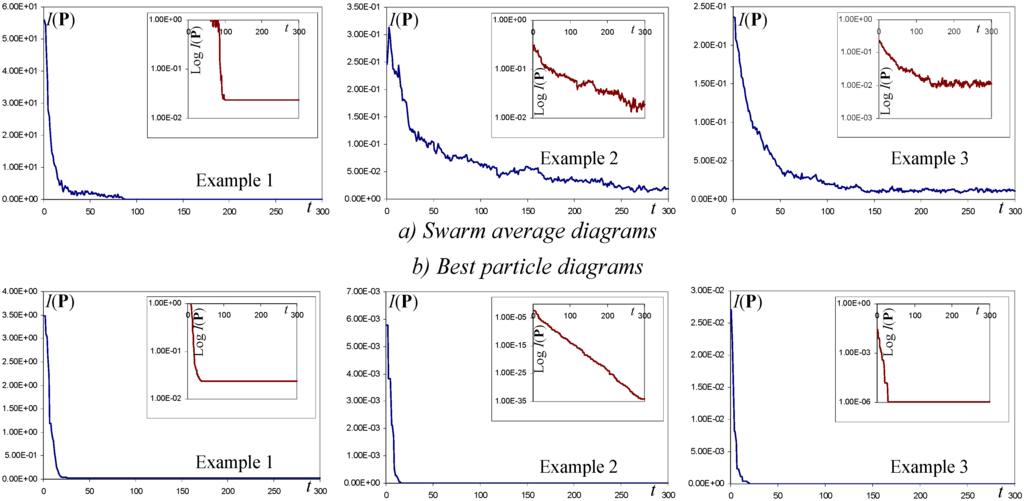
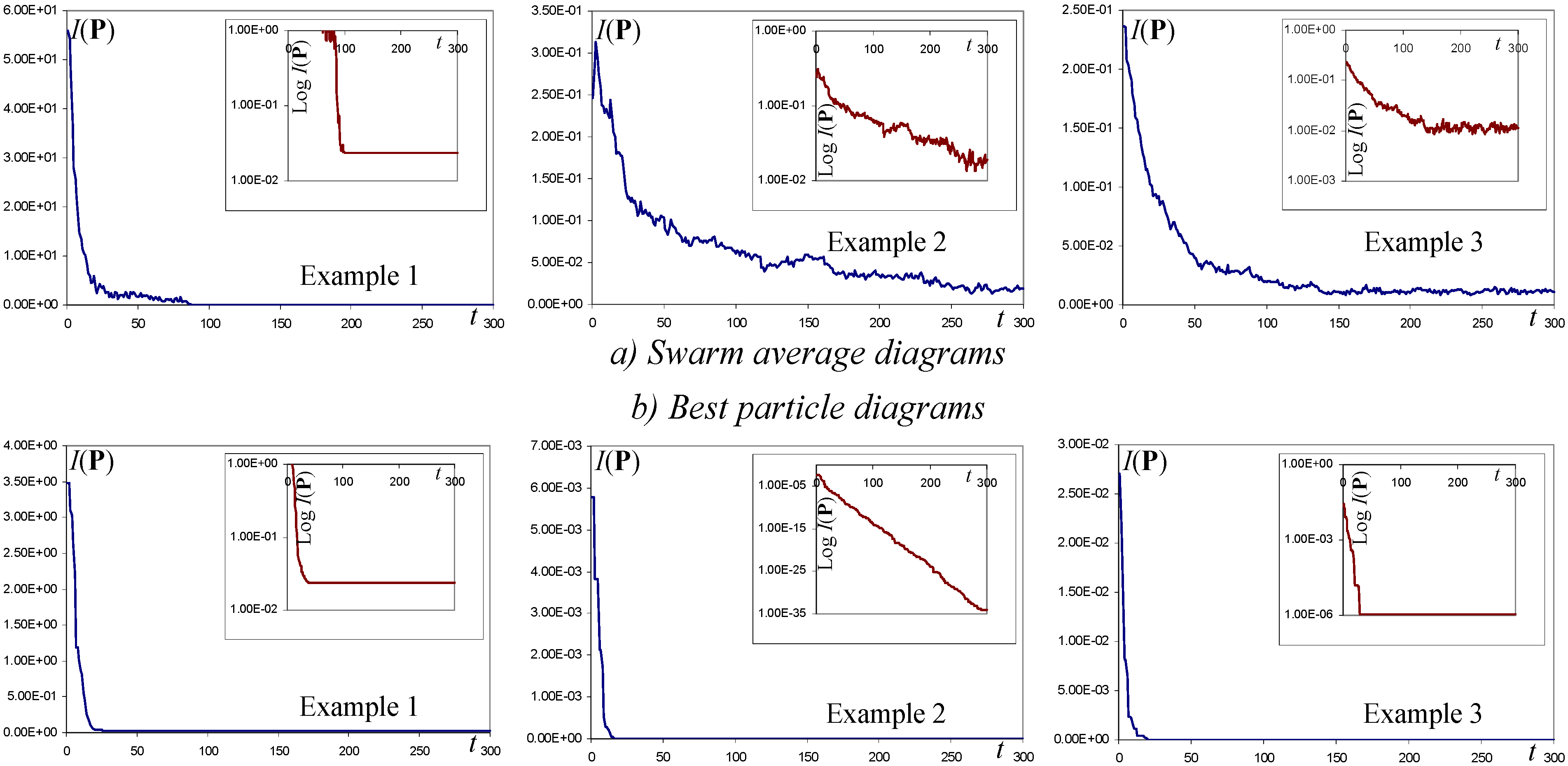
Figure 8. Convergence diagrams of I(P) for the three examples (in small, the diagrams in log-scale).

Figure 8. Convergence diagrams of I(P) for the three examples (in small, the diagrams in log-scale).

In other words, if the value of the parameters must be determined to within a precision of the order 10⁻²÷10⁻³, it can be a problem to determine the best choice of the parameters for a given problem, or, which is the same, how much changes of these parameters condition the result? So, the choice to use evolving parameters can be a better strategy, as the fact that their value changes along the iterations do not force the user to a precise choice and ensures him to have a good compromise between exploration and exploitation.

A last consideration concerns the convergence of the computations; in Fig. 8 the diagrams of convergence of the swarm average and best particle are shown for the three examples above; the diagrams are those of the run containing the best solution found in each case.

In the case of example 2, the log-scale diagrams are almost linear, especially the diagram of the best particle; this is the case of the lowest value of the residual. A linear decrease in log-scale means that the order of magnitude of the residual is linearly decreased along iterations. This seems to be an optimal situation for computations, but unfortunately it is strongly problem-dependent, as diagrams of examples 1 and 3 show. Nevertheless, suitable trajectories of the parameters c₀, c₁ and c₂ can be found for each problem to push the convergence log-diagrams towards linearity. This should be a guideline for users in the search of a good trajectory for a given problem.

The main advantage of the algorithm ALE-PSO remains the fact that the possibility to let evolve each parameter independently from the others give to the user a wide choice of possible trajectories that can be, with a few essays, tuned for the problem at hand, in such a way to find a good trade-off between exploration and exploitation, and this without the need to determine them with a high precision. In other words, the tricky problem of fine tuning the parameters for a given problem is bypassed by the choice, less difficult and needing less precision, of a suitable trajectory.

References

- Eberhart, R. C.; Kennedy, J. Particles swarm optimization. In Proc. of IEEE International Conference on Neural Networks, Piscataway, NJ, 1995; pp. 1942–1948.
- Shi, Y.; Eberhart, R. C. Parameter selection in particle swarm optimization. In Proc. of 7th Annual conference on Evolution Computation, New York, NY, 1998; pp. 591–601.
- Ozcan, E.; Mohan, C. K. Particle swarm optimization: surfing the waves. In Proc. of IEEE Congress on Evolutionary Computation, Washington DC, 1999; pp. 1939–1944.
- Clerc, M.; Kennedy, J. The particle swarm: explosion, stability and convergence in a multi-dimensional complex space. IEEE Transactions on Evolutionary Computation 2002, 6, 58–73. [Google Scholar] [CrossRef]
- Trelea, I. C. The particle swarm optimization algorithm: convergence analysis and parameter selection. Inform Proc Lett. 2003, 85, 317–325. [Google Scholar] [CrossRef]
- Liu, H.; Abraham, A.; Clerc, M. Chaotic dynamic characteristics in swarm intelligence. Appl Soft Comp. 2007, 7, 1019–1026. [Google Scholar] [CrossRef]
- Jiang, M.; Luo, Y. P.; Yang, S. Y. Stochastic convergence analysis and parameter selection of the standard particle swarm optimization algorithm. Inform Proc Lett. 2007, 102, 8–16. [Google Scholar] [CrossRef]
- Hu, X.; Eberhart, R. C. Adaptive particle swarm optimization: detection and response to dynamic systems. In Proc. of IEEE Congress on Evolutionary Computation, Hawaii, 2002; pp. 1666–1670.
- Yasuda, K.; Ide, A.; Iwasaki, N. Adaptive particle swarm optimization using velocity information of swarm. In Proc. of IEEE International Conference on Systems, Man & Cybernetics, The Hague, Netherlands, 2004; pp. 3475–3481.
- Yamaguchi, T.; Iwasaki, N.; Yasuda, K. Adaptive particle swarm optimization using information about global best. Elect Engin in Japan 2007, 159, 270–276. [Google Scholar] [CrossRef]
- DeBao, C.; ChunXia, Z. Particle swarm optimization with adaptive population size and its application. Appl Soft Comp. 2009, 9, 39–48. [Google Scholar]
- Vannucci, P. Designing the elastic properties of laminates as an optimisation problem: a unified approach based on polar tensor invariants. Int J of Struct and Multid Optim. 2006, 31, 378–387. [Google Scholar] [CrossRef]
- Verchery, G. Les invariants des tenseurs d'ordre 4 du type de l'élasticité. In Proc. of Euromech 115; 1979. Published by Editions du CNRS: Paris, 1982; pp. 93–104. [Google Scholar]
- Vannucci, P.; Vincenti, A. The design of laminates with given thermal/hygral expansion coefficients: a general approach based upon the polar-genetic method. Compos Struct. 2007, 79, 454–466. [Google Scholar] [CrossRef]
- Vannucci, P. A special planar orthotropic material. Jnl of Elast. 2002, 67, 81–96. [Google Scholar] [CrossRef]
- Vannucci, P. Plane anisotropy by the polar method. Meccanica 2005, 40, 437–454. [Google Scholar] [CrossRef]
- Miki, M. Material design of composite laminates with required in-plane elastic properties. In Proc. of ICCM 4, Tokio, 1982; pp. 1725–1731.
- Miki M. Design of laminated fibrous composite plates with required flexural stiffness. In Recent advances in composites in the USA and Japan; Vinson, J. R.; Taya, M. (Eds.) ASTM STP 864; ASTM: Philadelphia, 1985; pp. 387–400.
- Tsai, S. W.; Hahn, H. T. Introduction to Composite Materials; Technomic: Basel, 1980. [Google Scholar]
- Vincenti, A.; Vannucci, P.; Verchery, G. Design of composite laminates as an optimization problem: a new genetic algorithm approach based upon tensor polar invariants. In Proc. of WCSMO 5 (Fifth World Congress on Structural and Multidisciplinary Optimization), Lido di Jesolo, Italy, 2003.
- Grédiac, M. A procedure for designing laminated plates with required stiffness properties. Application to thin quasi-isotropic quasi-homogeneous uncoupled laminates. J. Composite Mat. 1999, 33, 1939–1956. [Google Scholar] [CrossRef]
- Vannucci, P. Influence of invariant material parameters on the flexural optimal design of thin anisotropic laminates. Int Jnl of Mech Sci. 2009, 51, 192–203. [Google Scholar] [CrossRef]
- Valot, E.; Vannucci, P. Some exact solutions for fully orthotropic laminates. Compos Struct. 2005, 69, 157–166. [Google Scholar] [CrossRef]
- Vannucci, P. Exact optimal flexural design of laminates. To appear in Compos Struct.; 2009. [Google Scholar] [CrossRef]
© 2009 by the authors; licensee Molecular Diversity Preservation International, Basel, Switzerland. This article is an open-access article distributed under the terms and conditions of the Creative Commons Attribution license (http://creativecommons.org/licenses/by/3.0/).