Article

A Heuristics-Guided Simplified Discrete Harmony Search Algorithm for Solving 0-1 Knapsack Problem

1
College of Computer and Information Sciences, Fujian Agriculture and Forestry University, Fuzhou 350002, China
2
Key Laboratory of Smart Agriculture and Forestry, Fujian Province University, Fuzhou 350002, China
*
Author to whom correspondence should be addressed.
Algorithms 2025, 18(5), 295; https://doi.org/10.3390/a18050295
Submission received: 4 March 2025 / Revised: 28 April 2025 / Accepted: 9 May 2025 / Published: 19 May 2025
(This article belongs to the Section Algorithms for Multidisciplinary Applications)

Abstract

:
The harmony search (HS) algorithm is a novel metaheuristic which has been widely used to solve both continuous and discrete optimization problems. In order to improve the performance and simplify the implementation of the HS algorithm for solving the 0-1 knapsack problem (0-1KP), this paper proposes a heuristics-guided simplified discrete harmony search (SDHS) algorithm which does not use random search operator and has only one intrinsic parameter, harmony memory size. The SDHS algorithm uses a memory consideration operator to construct a feasible solution, and then the constructed solution is further enhanced by a solution-level pitch adjustment operator. Two heuristics, the profit–weight ratio of an item and the profit of an item, are used to greedily guide the memory consideration operator and the solution-level pitch adjustment operator, respectively. In the memory consideration operator, items are considered in non-ascending order of profit–weight ratio assigned from the harmony memory. In the solution-level pitch adjustment operator, items not in the knapsack are attempted to be selected in non-ascending order of profit. The SDHS algorithm outperforms several state-of-the-art algorithms, with an average improvement of 0.55% in the quality of solutions on large problem instances.

1. Introduction

The knapsack problem (KP) is a classical combinatorial optimization problem with diverse applications across numerous fields. Over time, KP has evolved into a family of variants, including the 0-1 Knapsack Problem (0-1KP), Multidimensional Knapsack Problem (MKP), Quadratic Knapsack Problem, and the Generalized Knapsack Sharing Problem. Among these, the 0-1KP, as the foundational formulation of KP, plays a critical role in both theoretical and applied contexts. For instance, it has been utilized in real estate maintenance optimization [1], energy consumption minimization [2], cargo loading optimization [3], cryptographic systems [4], network security interdiction [5], and portfolio selection strategies [6]. These applications underscore the versatility of the 0-1KP in addressing complex resource allocation challenges under constraints.
The 0-1KP is NP-hard, necessitating the development of advanced metaheuristics to approximate optimal solutions [7]. Prominent examples of these metaheuristics include the cuckoo search algorithm [8,9,10], firefly algorithm [10], social spider algorithm [11], cohort intelligence algorithm [12], monkey algorithm [13], wolf-inspired algorithms [14,15,16,17,18], bat algorithm [19], wisdom of artificial crowds algorithm [20], symbiotic organisms search algorithm [21], elite opposition-flower pollination algorithm [22], chemical reaction optimization algorithm [23,24], genetic algorithm [25,26], monarch butterfly optimization algorithm [27,28,29], particle swarm optimization algorithm [30], whale optimization algorithm [31], shuffled frog leaping algorithm [32,33], slime mold algorithm [34], rice optimization algorithm [35], Differential Evolution algorithm [36], Quadratic Interpolation Optimization algorithm [36], Manta Ray Foraging Optimization algorithm [36], Artificial Jellyfish Search algorithm [37], Kepler Optimization Algorithm [38], harmony search algorithm [39,40,41,42,43,44,45,46], local search algorithm [47,48,49], etc. Most of the aforementioned algorithms require additional transfer functions to obtain binary solutions from continuous search space, use a hybrid of multiple metaheuristics, use advanced computation technologies, use enhanced operators, and/or use extra operators. Take the five cuckoo search algorithms [8,9,10,50,51] as an example: (1) all those five algorithms use the Sigmoid function to transfer a real number into binary; (2) ref. [50] uses the genetic mutation operation to prevent it from being trapped in the local optimum; (3) ref. [51] uses a hybrid of the cuckoo search algorithm and shuffled frog-leaping algorithm; (4) ref. [9] uses a hybrid of the cuckoo search algorithm and harmony search; and (5) ref. [10] uses the stochastic hill-climbing technique to improve its intensification ability. Although those advanced strategies are helpful to obtaining good performance, they give rise to extra complexity also.
The harmony search (HS) algorithm [52] is a kind of construction-based metaheuristic which was proposed to solve both continuous and combinatorial optimization problems. Inspired by the music improvisation process, the HS algorithm uses three operators, memory consideration operator, random search operator, and pitch adjustment operator, to construct a solution [53]. Since its publication, many improved HS algorithms have been proposed and successfully applied to many real-world optimization problems [54,55,56,57,58,59]. Several HS algorithms [39,40,41,42,43,44,45,46] have been successfully proposed to solve the 0-1KP. As stated in [60] and [61], the performance of the HS algorithm is remarkably affected by its parameters, and it is annoying to fine-tune those parameters. In order to further improve the performance and simplify the implementation of the HS algorithm for solving the 0-1KP, this paper proposes a heuristics-guided simplified discrete harmony search (SDHS) algorithm which does not use random search operator and has only one intrinsic parameter, harmony memory size (hms). The proposed SDHS algorithm uses the memory consideration operator to construct a feasible solution, and then the constructed solution is enhanced by a novel solution-level pitch adjustment operator. Two heuristics, the profit–weight ratio ( p i / w i ) of an item and the profit ( p i ) of an item, are used to greedily guide the memory consideration operator and the solution-level pitch adjustment operator, respectively. In the memory consideration operator, items are considered in non-ascending order of p i / w i to be assigned values from the harmony memory (HM). In the solution-level pitch adjust operator, items not in the knapsack are tried to be selected in non-ascending order of p i . Both the memory consideration operator and the solution-level pitch adjustment operator are carried out under the restriction of capacity constraint (2). Three experiments are performed to analyze the effect of the parameter hms on the performance, the convergence, and the diversity of the SDHS algorithm. Comparative experiments, conducted on three sets of large-scale 0-1KP instances, have shown that the SDHS algorithm performs better than other state-of-the-art metaheuristics.
The rest of this paper is organized as follows. Section 2 provides a short description of the basic HS algorithm and the existing HS algorithms for the 0-1KP. Section 3 presents the proposed SDHS algorithm for the 0-1KP. Section 4 analyzes the effect of the strategies and the parameter hms on the performance of the SDHS algorithm. Section 5 compares the performance of the SDHS algorithm with other state-of-the-art metaheuristics on three sets of large-scale 0-1KP instances. Finally, in Section 6, we summarize our study.

2. Preliminaries

2.1. Problem Formulation

Given a knapsack with maximum capacity W and a set of n items where each item i has a profit p i and a weight w i , the objective of the 0-1KP is to pack the knapsack with items such that a maximum profit is obtained under the constraint that the total weight of the items in the knapsack does not exceed the capacity of the knapsack. Mathematically, the 0-1KP can be modeled as the following 0-1 integer programming problem:
max f ( x ) = i = 1 n p i x i
                        s . t . i = 1 n w i x i W
                                                              x i 0 , 1
where x i indicates whether item i is packed in the knapsack. If  x i is equal to 1, then item i is packed in the knapsack; otherwise, it is discarded. Constraint (2) is the capacity constraint which guarantees that the total weight of the items in the knapsack is not greater than the knapsack’s capacity, and constraint (3) is the whole constraint which guarantees that no item is broken.

2.2. The Harmony Search Algorithm

The HS algorithm is a metaheuristic that mimics the improvisation process of music players to obtain better harmony. The basic HS algorithm uses three operators, i.e., the memory consideration operator, the pitch adjustment operator, and the random search operator, to cooperatively construct a new solution.
Given a solution represented as a vector x with n elements, Algorithm 1 describes the steps of the basic HS algorithm, in which lines 4 to 13 are used to construct a new solution x n e w until the stop condition is met (i.e., the maximum number of iterations or no improvement for certain iterations). Line 6, line 8, and line 11 are the memory consideration operator, the pitch adjustment operator, and the random search operator, respectively. In line 14, the newly produced solution x n e w is used to update the harmony memory if necessary.
Algorithm 1 The basic HS algorithm.
  1: Initialize the parameters of the HS algorithm
  2: Initialize the harmonies (solutions) in harmony memory
  3: while Stop condition is not met do
  4:     for each dimension j from 1 to n do
  5:         if rand() < hmcr then
                  // Memory Consideration Operator
  6:             x j n e w = x j i , where i is randomly selected from 1 to hms
  7:            if rand() < par then
                     // Pitch Adjustment Operator
  8:                Adjust x j n e w
  9:            end if
 10:       else
                  // Random Search Operator
 11:            Randomly create a value for x j n e w
 12:       end if
 13:    end for
 14:    Use x n e w to update harmony memory
 15:  end while
The HS algorithm stores several historical solutions in the harmony memory (HM), which can be represented by a matrix as Equation (4):
H M = x 1 1 x 2 1 x n 1 1 x n 1 x 1 2 x 2 2 x n 1 2 x n 2 x 1 h m s 1 x 2 h m s 1 x n 1 h m s 1 x n h m s 1 x 1 h m s x 2 h m s x n 1 h m s x n h m s
where hms is a parameter which represents the size of the harmony memory, and n is the number of decision variables of the problem at hand. Except for the hms, the basic HS algorithm has two additional intrinsic parameters, harmony memory consideration rate (hmcr) and pitch adjustment rate (par), which control the probability of selecting a solution component from the harmony memory and the probability of enhancing the selected component, respectively.
The basic HS algorithm is a general framework which may be implemented as continuous HS (CHS) algorithm or discrete HS (DHS) algorithm. For the CHS algorithm, another parameter b w , which represents an arbitrary distance bandwidth, is introduced to implement the pitch adjustment operator as the following:
x j n e w = x j n e w ± r a n d ( ) × b w
In order to implement random search operator for the CHS algorithm, the value of x j n e w can be randomly created as the following:
x j n e w = x j , m i n + r a n d ( ) × ( x j , m a x x j , m i n )
where x j , m i n and x j , m a x represent the minimum value and the maximum value of the jth dimension, respectively. For the implementation of the DHS algorithm, the random search operator can simply select a new value from all possible values for x j n e w , and the pitch adjustment operator may be abolished or redesigned according to the characteristics of the optimization problem at hand.
Both the CHS algorithm and the DHS algorithm can be used to solve the combinatorial optimization problem. In the field of the 0-1KP, the novel global harmony search (NGHS) algorithm [39] and the harmony search algorithm based on teaching–learning strategies (HSTL) [43] belong to the CHS algorithm. In order to use the CHS algorithm for the 0-1KP, a mapping strategy must be specified to map a real number into 0 or 1. In the NGHS algorithm, because the position updating equations are defined for real numbers in the range of 0 to 1, every variable is replaced by the nearest integer to obtain 0 or 1. Same strategy is used by the HSTL algorithm to obtain binary solution from continuous variables. The adaptive binary harmony search (ABHS) algorithm [41], the binary modified harmony search (BMHS) algorithm [42], the discrete global best harmony search (DGHS) algorithm [44], and the simplified binary harmony search (SBHS) algorithm [45] belong to the DHS algorithm. We introduce these DHS algorithms in detail in the next subsection.

2.3. Discrete HS Algorithms for the 0-1KP

In the ABHS algorithm [41], two strategies, the bit selection strategy and the individual selection strategy, are designed to implement the memory consideration operator. The bit selection strategy implements the classical memory consideration operator, and the individual selection strategy implements a new memory consideration operator as the following:
x j n e w = x j p , if r a n d ( ) < h m c r r o u n d ( r a n d ( ) ) , otherwise
where x p is a random harmony which is fixed for all items of x n e w , and the round function rounds a number to the nearest integer. The random search operator of the ABHS algorithm randomly selects a new value (0 or 1) for x j n e w . The pitch adjustment operator of the ABHS algorithm is designed to learn from the global best harmony with probability par.
In the BMHS algorithm [42], the pitch adjustment operator is designed to learn from the global best harmony or to produce a new value randomly as the following:
x j n e w = x j b e s t , if r a n d ( ) < 0.5 r o u n d ( r a n d ( ) ) , otherwise
where x b e s t is the best harmony in the harmony memory. The random search operator of the BMHS algorithm randomly selects a new value (0 or 1) for x j n e w .
In order to enhance the local search ability of HS algorithm for the 0-1KP, the DGHS algorithm [44] heavily uses the best harmony to guide the improvisation of new solution. In the DGHS algorithm, a new solution is improvised as the following:
x j n e w = x j b e s t , if r a n d ( ) < h m c r x j i , otherwise
where x b e s t is the best harmony in the harmony memory, and x i is randomly selected from the harmony memory. Furthermore, the  x j n e w , which is not selected from x j b e s t , is flipped with probability par.
In order to appropriately balance the intensification and diversification of the HS algorithm, the SBHS algorithm [45] proposes an ingenious improvisation scheme as the following:
x j n e w = x j r 1 + ( 1 ) x j r 1 × ( x j b e s t x j r 2 ) , j { 1 , 2 , , n }
where r 1 and r 2 are two distinct random integers between 1 and hms for each dimension j. Equation (10) combines the memory consideration and the pitch adjustment to improvise each bit of a new harmony, so the SBHS algorithm does not need parameter par. On the right-hand side of Equation (10), the first term represents the memory consideration operator, and the second term represents the pitch adjustment operator. The exclusive OR of x j b e s t and x j r 2 determines the value of x j n e w . If  x j b e s t x j r 2 is equal to 0, then x j r 1 is assigned to x j n e w directly; otherwise, 1 x j r 1 is assigned to x j n e w . The SBHS algorithm has only two parameters, i.e., hms and hmcr, which greatly simplifies the fine-tuning of parameters.

3. Simplified Discrete Harmony Search Algorithm for the 0-1KP

The HS algorithm is a simple, effective, and flexible metaheuristic for both continuous and discrete optimization problems. Among the three components of the HS algorithm, the memory consideration operator, which learns from historical experience stored in the harmony memory, is the core component. The other two components, the pitch adjustment operator and the random search operator, are designed to enhance its intensification ability and enlarge its diversification, respectively.
The cooperation of these two components can obtain good balance between exploration and exploitation for the HS algorithm. Although the basic HS algorithm is both simple and easy to implement, to design an HS algorithm with excellent performance for a specific problem is far from a simple task.
Based on the characteristics of the problem at hand, we must analyze the three components of the basic HS algorithm carefully to answer the following two questions: (1) whether a component is needed for the problem at hand, and (2) how to implement this component if it is needed. The 0-1KP has the following two characteristics. One is that each variable has only two possible values, i.e., 0 or 1. The other is that an item with a high profit–weight ratio or profit should be picked with high priority. Based on these two key characteristics of the 0-1 knapsack problem (0-1KP), the necessity and implementation details of the memory consideration operator, pitch adjustment operator, and random search operator are explored in the following subsections.

3.1. Discussions of the HS Algorithm

The main purpose of the random search operator is to maintain enough diversity for the HS algorithm to have an optimization ability even in the late stage of the search. To obtain this objective, the CHS algorithm uses Equation (6) to randomly create a new value for x j n e w . The 0-1KP is a discrete optimization problem where the value of x j n e w can only be 0 or 1. Consequently, x j , m i n and x j , m a x are 0 and 1, respectively. A possible implementation of the random search operator is to randomly select a value from {0,1} for the x j n e w with probability 1-hmcr, so both 0 and 1 can have a chance to be the value of x j n e w . As a result, Equation (6) can be rewritten as represented as Equation (11):
x j n e w = x j , m i n + r a n d ( ) × ( x j , m a x x j , m i n ) = 0 + r a n d ( ) ( 1 0 ) { 0 , 1 }
In the case of the 0-1KP, the HM maintains a repository of historical solutions. Let HM ( j ) denote the historical solutions corresponding to the j-th dimension. When the harmony memory contains a sufficient number of solutions, new values x j n e w can be directly retrieved from HM ( j ) as shown in Equation (12). This approach achieves comparable outcomes to the random search operator, thereby rendering the parameter hmcr obsolete. Consequently, the random search operator is eliminated, and each x j n e w is consistently selected from the harmony memory:
x j n e w HM ( j ) = x j 1 x j 2 x j h m s 1 x j h m s
The pitch adjustment operator of the standard HS aims to improve its local search ability. The classical pitch adjustment operator is implemented at the dimension level, and the binary solution space such as 0-1KP, bw for the pitch adjustment operator is 1, and thus x j n e w can be adjusted according to Equation (13):
x j n e w = ( x j n e w ± r a n d ( ) × b w ) { 0 , 1 }
As noted by Wang et al. in [41], the pitch adjustment operator of the HS algorithm is degenerated in the binary space, necessitating the development of a new approach to enhance its intensification ability. In solving the 0-1KP, most metaheuristics employ a greedy optimization operator to refine solutions. Unlike the classical pitch adjustment operator, which operates at the dimension level, the greedy optimization functions at the solution level. Specifically, for a n-dimensional solution x = ( x 1 , x 2 , , x n ) , the new solution x n e w is generated by applying a greedy optimization operator Opt ( · ) as defined in Equation (14):
x n e w = Opt ( x )
Given that the greedy optimization operator substantially strengthens the intensification capability, the classical pitch adjustment operator is no longer required for the 0-1 knapsack problem (0-1KP) and is therefore omitted.
In the 0-1KP, the capacity constraint of the knapsack introduces an indirect competitive relationship among items. For instance, incorporating an item α with profit p α and weight w α may hinder the inclusion of another item β (with profit p β and weight w β ) due to the limited capacity. To address this, we evaluate items based on their profit-to-weight ratio ( p w ) or individual profit, where p w is defined as Equation (15):
p w j = p j w j
Given that the primary objective of the 0-1KP is to maximize profit, the memory consideration operator processes items in non-ascending order of their profit-to-weight ratio or individual profit.

3.2. Description of the SDHS Algorithm

Accordingly, based on the aforementioned analysis, the random search operator is omitted from our SDHS algorithm. Consequently, the memory consideration operator prioritizes items based on their profit-to-weight ratio p w , while the pitch adjustment operator is executed at the solution level. In the subsequent subsections, we detail the memory consideration operator, the solution-level pitch adjustment mechanism, and the comprehensive framework of the SDHS algorithm. And the pseudo code of the proposed SDHS algorithm for 0-1KP is provided in Algorithm  2. Figure 1 shows the flowchart of the SDHS algorithm.
Algorithm 2 Pseudo code of the SDHS algorithm for the 0-1KP.
Require:    m , h m s
Ensure:  best solution found;
  1:  Initialize every x i for the harmony memory, where i { 1 , 2 , , h m s }
  2:   b e s t the best harmony in harmony memory
  3:  while  m > 0  do
                  //Memory consideration
  4:      Call Algorithm 3 to construct a solution x n e w
                  //Pitch adjustment
  5:      Call Algorithm 4 to enhance the solution x n e w
                  //Update the harmony memory
  6:      if  x n e w is better than the worst solution in the harmony memory then
  7:         Remove the worst solution in the harmony memory
  8:         Append x n e w into the harmony memory
  9:      end if
 10:     if  x n e w is better than b e s t  then
 11:          b e s t = x n e w
 12:     end if
 13:       m = m 1
 14:  end while
 15:  return  b x
As shown in Algorithm  2, parameters m and h m s represent the maximum generation of the SDHS algorithm and the size of the harmony memory. The initial solutions in the harmony memory are randomly created. The initialization of the harmony memory requires the random initialization of n items of the heap h m s of harmonies, and its time complexity is O ( h m s × n ) . In line 4, the SDHS algorithm calls the memory consideration operator to construct a new solution x n e w . In line 5, the SDHS algorithm calls the solution-level pitch adjustment operator to improve the solution x n e w . Lines 6 to 9 are used to update the harmony memory. We can use a heap to implement the harmony memory, so the time complexity to maintain the harmony memory is O ( log 2 h m s ) . Lines 10 to 12 are used to record the best solution. Because of the time complexity of both Algorithms 3 and 4 is O ( n ) , the time complexity to construct a solution and maintain the harmony memory is O ( n + log 2 h m s ) . In Algorithm 2, m solutions are constructed in total, so the time complexity of the SDHS algorithm is O ( h m s × n + m × ( n + log 2 h m s ) ) .
As illustrated in Table 1, a comparison is made between the time complexity and parameter settings of basic HS and SDHS. It is evident that both algorithms exhibit analogous initialization and memory consideration complexities. The adoption of a heap structure by SDHS results in a reduction in the complexity of the harmony memory update process from O ( h m s ) to O ( log 2 h m s ) . The algorithm’s enhanced adaptability and usability is attributable to the simple, flexible, and efficient operator design, which retains only a single parameter ( h m s ).
To facilitate the comparative study of metaheuristics for the 0-1KP, the source code of the SDHS algorithm has been made publicly available in GitHub (https://github.com/1497135676/SDHS4KP (accessed on 8 May 2025)).

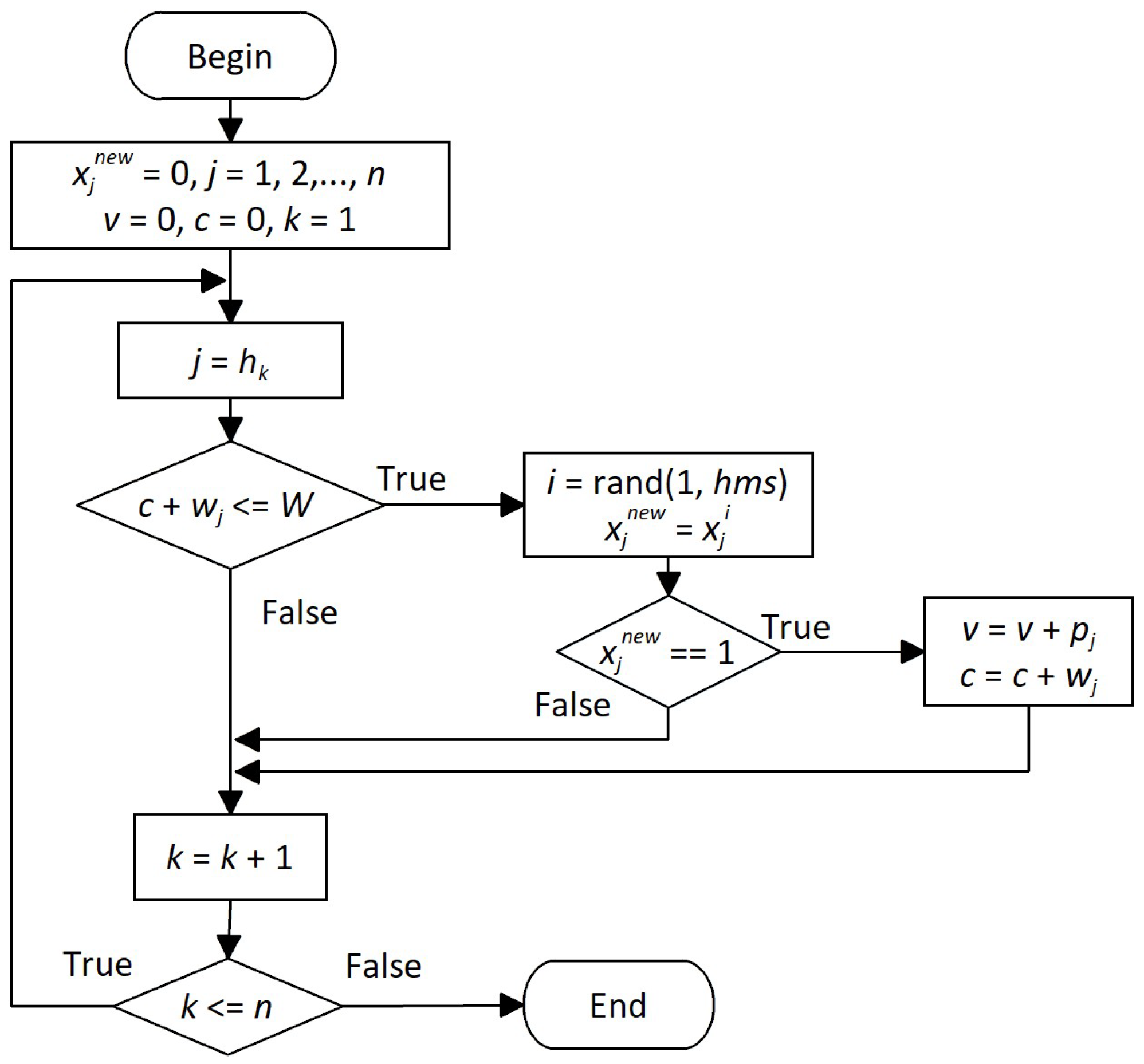
3.3. Memory Consideration Operator

Algorithm  3 is the memory consideration operator which is used to construct a feasible solution from scratch. In Algorithm  3, items are processed in non-ascending order of the profit–weight ratio under the constriction of the capacity constraint. This heuristic-guided strategy has been widely used by other metaheuristics, such as [13,21,23,24,44,45], to design the greedy repair operator to repair an infeasible solution.
Algorithm 3 The memory consideration operator.
  1:   x j n e w = 0 , for  j = 1 , 2 , . . . , n
  2:   v = 0
  3:   c = 0
  4:  for  k = 1 to n do
  5:       j = h k
  6:      if  c + w j W  then
  7:          Randomly select a harmony x i from the harmony memory
  8:           x j n e w = x j i
  9:          if  x j n e w = = 1  then
 10:              v = v + p j
 11:              c = c + w j
 12:         end if
 13:     end if
 14:  end for
In Algorithm 3, variable x n e w is a vector which represents the new constructed solution. Each element x j n e w of x n e w indicates whether item j is in the knapsack. In the first line of Algorithm 3, each element of x n e w is set to 0, which means no item is selected in the beginning. Variable v and variable c represent the total profit and the total weight of the items in the knapsack, respectively. Variable h is a vector which stores the items in non-ascending order of the profit–weight ratio. From line 4 to line 14 of Algorithm  3, items are processed in non-ascending order of the profit–weight ratio. If the selection of an item j does not violate the capacity constraint, then a harmony x i is randomly selected from the harmony memory and the value of x j i is assigned to x j n e w . If the value of x j n e w is equal to 1, which means item j is selected, then the profit and weight of item j is added to v and c, respectively. Apparently, the constructed solution is a feasible solution, and the time complexity of Algorithm  3 is O ( n ) . Figure 2 is the corresponding flowchart.

3.4. Solution-Level Pitch Adjustment Operator

In the field of 0-1KP, the greedy optimization method has been widely used to enhance the feasible solution. Most of the existing metaheuristics, such as [13,21,23,24,44,45], use only the profit–weight ratio to guide the greedy optimization method. Our studies in using trajectory-based metaheuristics for the 0-1KP [47,48] have found that profit information can provide an extra intensification ability for the greedy optimization method. In the SDHS algorithm, we use a profit-guided greedy optimization method, where only profit is used to rank the items. The profit-guided greedy optimization method can be regarded as a solution-level pitch adjustment operator which is used to replace the classical dimension-level pitch adjustment operator of the HS algorithm. Algorithm 4 is the pseudo code of the solution-level pitch adjustment operator.
Algorithm 4 Solution-level pitch adjustment operator.
Require:  x , v , c //A feasible solution
  1:   h the sorted items in non-ascending order of profit
  2:  for  k = 1 to n do
  3:       j = h k
  4:      if  x j = = 0 and c + w j W  then
  5:           x j = 1
  6:           v = v + p j
  7:           c = c + w j
  8:      end if
  9:  end for
10:  return  x , v , c
In Algorithm 4, parameters x, v, and c represent a feasible solution, the total profit of the selected items in solution x, and the total weight of the selected items in solution x, respectively. Variable h is a vector which stores the items in non-ascending order of profit. The solution-level pitch adjustment operator examines each item j in non-ascending order of profit and changes x j from zero to one if the selection of item j does not violate the capacity constraint. Because each item must be checked for whether it can be put into the knapsack to enhance the solution, the time complexity of Algorithm 4 is O ( n ) .

4. Behavior Analysis

In the SDHS algorithm, parameter m controls the maximum number of solutions constructed. Changing this parameter leads to different trade-offs between the solution quality and computation resource used. In the LBSA algorithm [47] and the NM algorithm [48], the maximum number of neighbor solutions is set to 40,000. Therefore, for a fair experimental analysis, the maximum number of solutions constructed by the SDHS algorithm is also set to 40,000.
Except parameter m, there is only one parameter ( h m s ) needed to be fine-tuned for the SDHS algorithm. The three types of 0-1KP instances used by [29] are used in this paper to find a suitable parameter h m s and analyze the behaviors of the SDHS algorithm. The features of the three types of instances are listed in Table 2.
Each type contains five 0-1 KP instances, and the numbers of items are 800, 1000, 1200, 1500, and 2000, respectively. These fifteen instances are called KP01, KP02, …, KP15, respectively. Among those fifteen instances, KP01 to KP05 are uncorrelated instances, KP06 to KP10 are weakly correlated instances, and KP11 to KP15 are strongly correlated instances. The six instances used in this F are KP01, KP04, KP08, KP09, KP14, and KP15. The principle of selecting these six instances is based on our former studies on the LBSA algorithm [47] and the NM algorithm [48]. We want to use difficult instances to tune the parameters of the SDHS algorithm. For uncorrelated instances, KP01 and KP04 are the two instances where the probability to find the best-known solution is less than 50 % . For weakly correlated instances, KP08 and KP09 are the two instances where the probability to find the best-known solution is less than 50 % . For strongly correlated instances, because both the LBSA algorithm and the NM algorithm can always find the best-known solutions for all instances, we select the two largest instances.

4.1. Effect of Heuristics and Parameter on Performance

The SDHS algorithm has the following three characteristics: (1) there is only one intrinsic parameter, i.e., harmony memory size hms; (2) the processing order of items in the memory consideration operator is guided by the profit–weight ratio of the item; and (3) the solution-level pitch adjustment operator is guided by the profit of the item. To observe the effect of parameter hms, the contribution of using the profit–weight ratio in the memory consideration operator, and the contribution of using the profit in the pitch adjustment operator, we compare the SDHS algorithm with two variants of the SDHS algorithm, i.e., the SDHS1 algorithm and the SDHS2 algorithm. In the SDHS1 algorithm, the processing order of items is not guided by the profit–weight ratio, which means the items are processed from the first item to the last item in sequence, like in the classical HS algorithm. The comparison between the SDHS algorithm and the SDHS1 algorithm can tell us whether there is positive effect to using the profit–weight ratio to guide the processing order of items. In the SDHS2 algorithm, the solution-level pitch adjustment operator is guided by the profit–weight ratio like the greedy optimization operator used in most metaheuristics for the 0-1KP. The comparison between the SDHS algorithm and the SDHS2 algorithm can tell us whether using the profit to guide the solution-level pitch operator is superior to using the profit–weight ratio.
To find a suitable hms for the SDHS algorithm and to compare the performance of the three SDHS algorithms, we test twenty different values for hms, from 100 to 2000 with a step 100. For each hms, we run the three SDHS algorithms 200 times on each instance and calculate the absolute error of the average profit. Table 3 lists the simulation results of the three SDHS algorithms on the two uncorrelated instances, Table 4 lists the simulation results on the two weakly correlated instances, and Table 5 lists the simulation results on the two strongly correlated instances.
Table 3 shows that the SDHS algorithm can always obtain the best-known solution on KP01 and KP04 when the hms is in the range of 500 to 2000 and in the range of 300 to 2000, respectively. Table 4 shows that the SDHS algorithm can always obtain the best-known solution on KP08 and KP09 when the hms is in the range of 300 to 2000 and in the range of 500 to 1200, respectively. Table 5 shows that the SDHS algorithm can always obtain the best-known solution on KP14 and KP15 when the hms is in the range of 100 to 900 and in the range of 100 to 700, respectively. The simulation results of the SDHS algorithm on these six instances show that (1) for each instance, the SDHS algorithm can always obtain the best-known solution in a wide range of hms, and (2) when parameter hms is set to 500, 600, or 700, the SDHS algorithm can always find the best-known solutions on all these six instances.
The simulation results in Table 3, Table 4 and Table 5 show that the SDHS1 algorithm can never obtain the best-known solution on any of the six instances. Apparently, the performance of the SDHS algorithm is far better than that of the SDHS1 algorithm. Because the only difference between the SDHS algorithm and the SDHS1 algorithm is the processing order of the items, it means that the profit–weight ratio-guided processing order plays an important role in the SDHS algorithm performing well.
Table 3 shows that the SDHS2 algorithm can always obtain the best-known solution on KP01 and KP04 when the hms is in the range of 1700 to 2000 and in the range of 300 to 2000, respectively. Table 4 shows that the SDHS2 algorithm can always obtain the best-known solution on KP08 and KP09 when the hms is in the range of 600 to 2000 and in the range of 400 to 2000, respectively. Table 5 shows that the SDHS2 algorithm can always obtain the best-known solution on KP14 when the hms is in the range of 400 to 1100. The simulation results of the SDHS2 algorithm on these six instances show that (1) there exists a range of parameter hms for the SDHS2 algorithm to always obtain the best-known solution on KP01, KP04, KP08, KP09, and KP14, respectively; (2) using the parameters in range of 100 to 2000, the SDHS2 algorithm can never obtain the best solution on KP15; and (3) even on the five instances except KP15, there is not a common hms for the SDHS2 algorithm to obtain the best-known solutions on all these five instances. These results indicate that the performance of the SDHS2 algorithm is not as good as that of the SDHS algorithm. Because the only difference between the SDHS algorithm and the SDHS2 algorithm is the heuristic used to guide the processing order of the items in the solution-based pitch adjustment operator, it means that, for the solution-based pitch adjustment operator, the profit-guided processing order is superior to the profit–weight ratio-guided processing order.
Zhao et al. [25] analyzed that only using the profit–weight ratio may fail to find the best solution for the construction method in some cases. Similarly, only using the profit–weight ratio may also fail to find best solution for metaheuristics in some cases. For example, suppose the remaining capacity of package is 30 and there are 3 items not in the package. The profits and weights of those three items are [20, 25, 25] and [10, 15, 15], respectively. Then, the profit–weight ratio of those three items are [2, 5/3, 5/3]. If the profit–weight ratio is used to guide the pitch adjustment operator, then the total profit will increase by 45. But if the profit is used to guide the pitch adjustment operator, then the total profit will increase by 50. In the SDHS algorithm, the memory consideration operator is guided by the profit–weight ratio, and the pitch adjustment operator is guided by the profit. These two heuristics cooperate with each other to guarantee good performance for the SDHS algorithm. To further experimentally analyze whether this result is reliable, we carry out comparative experiment on six types of 0-1KP instances with a wide range of parameters. The six types include uncorrelated (UC), weakly correlated (WC), strongly correlated (SC), multiple strongly correlated (MSC), profit ceiling (PC), and circle (CI) instances. The weights are distributed in [1, R] where R is in 100, 1000, 10,000. The profits are created according to the type of instance [62]. The value of n (number of items) is from 1000 to 2000 with a step of 100. For each combination of type, R, and n, 10 instances are created. In total, 1980 instances ( 6 × 3 × 11 × 10 ) are used in the comparative experiment. For each instance, we run the methods 50 times and use the mean value to compare the performance of using profit and using profit–weight ratio. Table 6 lists the statistical values of the experimental results, where columns >, =, and < list the number of instances where using profit has better, equal, or worse performance, respectively. Column p-value lists the results of the Wilcoxon signed ranks test which is highlighted in bold if using profit is significantly better than using profit–weight ratio. In case the two strategies obtain exactly same results on 110 instances, the corresponding cells of p-value are labeled as ‘-’. Among the 18 combination of type and R, using profit is significantly better than using the profit–weight ratio on 12 cases, has no significant difference on 5 cases, and is significantly worse only on 1 case when the type is PC and R is 10,000. These results confirm that using the profit to guide the solution-level pitch adjustment operator is superior to using the profit–weight ratio.

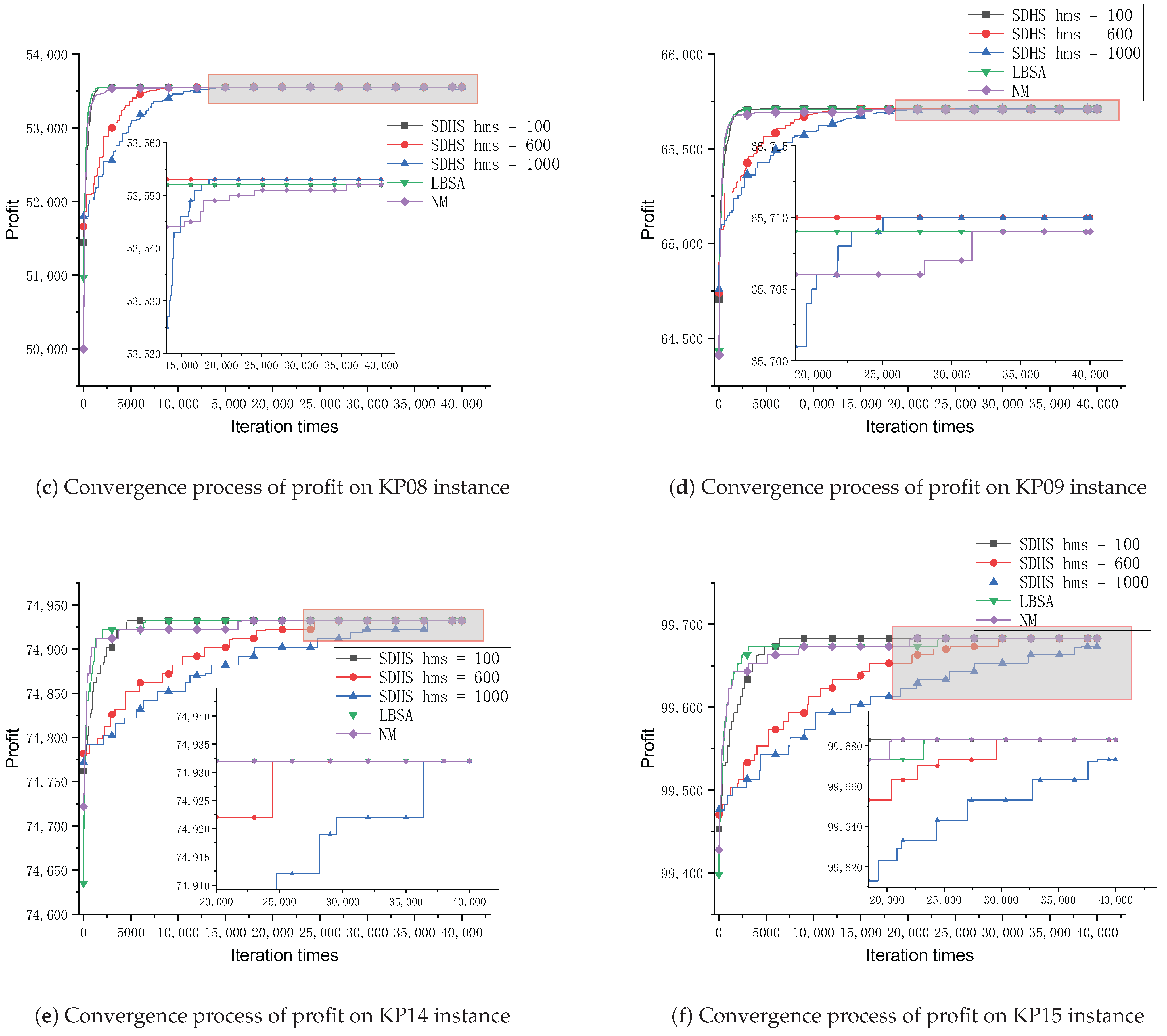
4.2. Effect of Parameter hms on the Convergence Process

To analyze the effect of parameter hms on the convergence process of the SDHS algorithm, we compare the convergence process of the SDHS algorithms with three different values of parameter hms, i.e., 100, 600, and 1000. Figure 3a–f show the convergence process of the SDHS algorithm on KP01, KP04, KP08, KP09, KP14, and KP15, respectively. Those figures clearly show that parameter hms controls the convergence speed of the SDHS algorithm. If parameter hms is too small, the selection pressure will be too strong, and then the convergence speed will be too quick, and it may lead to premature convergence easily. On the contrary, if parameter hms is too large, the selection pressure will be too weak, and then the convergence speed will be too slow, and it may lead to insufficient exploitation. A suitable parameter hms is important for the SDHS algorithm to have good convergence behavior.

4.3. Effect of Parameter hms on the Diversity

To analyze the effect of parameter hms on the diversity of the SDHS algorithm, we use the entropy of the solutions in harmony memory to measure the diversity of the SDHS algorithm, and compare the entropy of the SDHS algorithms with three different values of parameter hms, i.e., 100, 600, and 1000. We use f j , 1 to represent the frequency when x j is equal to 1, and use f j , 0 to represent the frequency when x j is equal to 0. Then, the entropy for the selection of item j can be defined as
H j = i = 0 1 f j , i log 2 ( f j , i )
The maximum of Equation (16) occurs when the selecting and discarding of the item j are equally likely. The minimum of Equation (16) occurs when all solutions select item j or no solution selects item j. That means a value of 1 represents the largest diversity for the selection of item j, and 0, no diversity. The entropy of the solutions in harmony memory is defined as the average of the H j :
H = j = 1 n H j n
where n is the number of items. Apparently, the value of H is between 0 and 1. When the H is equal to 1, the SDHS algorithm has the largest diversity. When H is equal to 0, the SDHS algorithm does not have any diversity and we cannot construct a new solution after that.
Figure 4a–f are the entropy of the SDHS algorithm on KP01, KP04, KP08, KP09, KP14, and KP15, respectively.
These figures clearly show that parameter hms controls the decrease speed of the entropy for the SDHS algorithm. As the entropy is used to measure the diversity, if parameter hms is too small, the decrease speed of diversity will be too quick and it may lead to premature convergence easily. On the contrary, if parameter hms is too large, the decrease speed of diversity will be too slow and it may lead to insufficient exploitation. A suitable parameter hms is important for the SDHS algorithm to have enough diversity.

4.4. The Running Time of SDHS

The significance of using the metaheuristic for the 0-1KP is that the time complexity and space complexity of the metaheuristic is independent of the capacity of package. As reported in [62], dynamic programming (DP) algorithms fail when the capacity of package is large, and branch and bound methods fail in difficult instances even with a small number of items, such as multiple strongly correlated, profit ceiling, and circle instances. There are numerous instances for which all currently known exact methods perform badly [62]. Using DP as an example, both its time complexity and space complexity are O ( n W ) , which means DP may run out of space if the capacity of package is large enough. Even if the memory is enough, due to the cost of managing large memory, the running time of DP may increase quickly if the capacity of package is large. We use a set of uncorrelated instances to compare the running time of SDHS and DP. The item number is set to 1000, and the weights are distributed in [1, R] where R begins from 1000 and increases linearly with a step 500. In our experiment, the maximum memory of JVM is set to 5G. Our experiment finds that when R is 3500, the DP fails due to running out of memory. Figure 5 compares the running time of SDHS and DP on instances with different parameter R. Figure 5 clearly shows that the running time of SDHS is independent of the capacity of package, but the running time of DP increases sharply when the capacity of package is large.

5. Comparative Experiments

To observe the competitiveness of the SDHS algorithm, the performance of the SDHS algorithm is compared with thirteen state-of-the-art algorithms on three sets of large-scale 0-1KP instances. These three instances have been widely used to evaluate the performance of 0-1 knapsack problem algorithms. Table 7 shows the main information for these three example groups. The performance test of SDHS on the hms parameter is discussed in detail in Section 3. We set hms = 600 as the setting for subsequent experiments, which can make SDHS maintain good diversity and convergence speed.
The first set of large-scale 0-1KP instances, which includes sixteen instances, was proposed by Kong et al. in [45]. The numbers of items of these sixteen instances are 100, 200, 300, 500, 700, 1000, 1200, 1500, 1800, 2000, 2600, 3000, 3500, 4900, 5800, and 6400, respectively. These sixteen instances are named LKP01–LKP16. For each instance, the profit of each item is randomly produced from [0.5, 1], its weight is randomly produced from [0.5, 2], and the capacity of the knapsack is equal to 0.75 times of the total weights of the items. Apparently, these sixteen instances belong to uncorrelated instances. The second set of large-scale 0-1KP instance includes three types of 0-1KP instances, i.e., uncorrelated instances, weakly correlated instances, and strongly correlated instances. Each type contains five 0-1KP instances, and the numbers of items are 800, 1000, 1200, 1500, and 2000, respectively. The third set of large-scale 0-1KP instance includes five types of 0-1KP instances, i.e., weakly correlated instances [51], strongly correlated instances [51], multiple strongly correlated instances [51], profit ceiling instances [51], and uncorrelated instances [45]. Each of the first two types contains five instances, and the numbers of items are 200, 300, 500, 800, and 1000, respectively. Each of the middle two types contains five instances, and the numbers of items are 300, 500, 800, 1000, and 1200, respectively. The last type contains four instances, and the numbers of items are 3000, 5000, 7000, and 10,000, respectively.
In Section 5.1, we use the first set of large-scale 0-1KP instances to compare the SDHS algorithm with three HS algorithms. In Section 5.2, we use the second set of large-scale 0-1KP instances to compare the SDHS algorithm with six state-of-the-art metaheuristics. In Section 5.3, we use the third set of large-scale 0-1KP instances to compare the SDHS algorithm with four state-of-the-art metaheuristics. The SDHS algorithm is coded with Java and conducted on an Intel Core i9-13900HX CPU (2.4 GHz), 16 GB of memory, and Windows 11.

5.1. Experiment on the First Set of Large-Scale 0-1KP Instances

Using the first set of large-scale 0-1KP instances, we compare the SDHS algorithm with three HS algorithms, the novel global harmony search (NGHS) algorithm [39], improved adaptive binary harmony search (ABHS) algorithm [41], and simplified binary harmony search (SBHS) algorithm [45]. In [45], the maximum numbers of iterations for these instances are set to 15,000, 15,000, 20,000, 20,000, 30,000, 30,000, 40,000, 40,000, 50,000, 50,000, 60,000, 80,000, 100,000, 120,000, 150,000, and 200,000. In the SDHS algorithm, the number of iterations is set to the value used by [45] or 40,000 if the value used by [45] is bigger than 40,000. It means that the SDHS algorithm only constructs 20 percent of the number of solutions constructed by its competitors on the largest instance.
As in [45], the SDHS algorithm is run 30 times for each instance. The statistical results of 30 independent runs are reported in Table 8. The best results are highlighted in bold. The data of [39,41,45] are taken from [45]. In terms of the worst value and mean value, the SDHS algorithm obtains better results than the other three algorithms on all sixteen instances. In terms of the best value, the SDHS algorithm finds a new best solution on nine instances, i.e., LKP07, LKP08, LKP09, LKP11, LKP12, LKP13, LKP14, LKP15, and LKP16. These results clearly show that the SDHS algorithm has best performance among the four HS algorithms.
In addition, the comparison results between SDHS and the average values of the competitive algorithms based on the Friedman test and Holm post hoc test are shown in Table 9. As shown in Table 9, according to the Friedman test, SDHS obtains the best ranking. Specifically, compared with NGHS and ABHS, SDHS has a significant advantage. Although the performance difference is not significant compared with the SBHS algorithm, SDHS obtains a better ranking, and the average values are all better than those of other algorithms. The table also counts the percentage of improvement of SDHS compared with the reported approach, calculated as Equation (18):
Gap ( A ) = Mean A Mean SDHS Mean A

5.2. Experiment on the Second Set of Large-Scale 0-1KP Instances

Using the fifteen large-scale 0-1KP instances introduced in Section 4, the SDHS algorithm is compared with six state-of-the-art metaheuristics, i.e., the hybrid cuckoo search algorithm with global harmony search (CSGHS) [9], binary monarch butterfly optimization (BMBO) algorithm [27], chaotic monarch butterfly optimization (CMBO) algorithm [29], opposition-based learning monarch butterfly optimization (OMBO) algorithm [28], list-based SA (LBSA) algorithm [47], and nosing method (NM) [48]. As in the LBSA algorithm and the NM, the maximum number of iterations is set to 40,000. The comparisons are listed in Table 10, Table 11 and Table 12, where the best results are highlighted in bold. Because the CSGHS algorithm and the BMBO algorithm are not tested on instances with 2000 items, the corresponding cells of those two algorithms are labeled as ‘-’.
Table 10 shows that the CSGHS algorithm and the BMBO algorithm cannot find the best-known solution on any instance. Both the CMBO algorithm and the OMBO algorithm cannot find the best-known solution on the KP03 instance. The NM cannot find the best-known solution on the KP01 instance. Both the LBSA algorithm and the SDHS algorithm can find the best-known solutions on all uncorrelated instances, but only the SDHS algorithm can always find best-known solutions. Table 11 shows that the CSGHS algorithm and the BMBO algorithm cannot find the best-known solution on any instance. The CMBO algorithm cannot find the best-known solution on the KP08 instance. Both the LBSA algorithm and the NM cannot find the best-known solution on the KP09 instance. Both the OMBO algorithm and the SDHS algorithm can find the best-known solutions on all weakly correlated instances, but only the SDHS algorithm can always find best-known solutions. Table 12 shows that the CSGHS algorithm and the BMBO algorithm cannot find the best-known solution on any instance. The CMBO algorithm cannot find the best-known solution on the KP12 instance. All the other four algorithms can find the best-known solutions on all strongly correlated instances, but only the NM, the LBSA algorithm and the SDHS algorithm can always find best-known solutions. In summary, only the SDHS algorithm can always find the best-known solutions on all 15 instances.
The comparison results between SDHS and the average values of the competitive algorithms, including CSGHS, BMBO, CMBO, OMBO, NM, and LBSA, are detailed in Table 13. These findings are derived from the Friedman test and Holm’s post hoc test, which provide a robust statistical framework for evaluating algorithmic performance. According to the Friedman test, SDHS achieves the highest ranking with a value of 1.71 , outperforming all other algorithms. Notably, SDHS exhibits a statistically significant advantage over CSGHS and BMBO. In contrast, when compared to CMBO, OMBO, NM, and LBSA, the performance differences are not statistically significant; nevertheless, SDHS consistently secures a superior ranking. The gap values further corroborate the dominance of SDHS: the smallest differences against NM and LBSA are 0.0005 , while larger gaps of 0.932 and 1.071 are observed against CSGHS and BMBO, respectively. Additionally, the comparison summary reveals no instances where SDHS underperformed relative to its counterparts as reflected by the ( + / = / ) notation sums (e.g., 0 / 0 / 12 for CSGHS and BMBO). Collectively, these results highlight the exceptional and consistent performance of SDHS across all evaluated scenarios, positioning it as a leading algorithm in this comparative analysis.

5.3. Experiment on the Third Set of Large-Scale 0-1KP Instances

Using the third set of large-scale 0-1KP instances, the SDHS algorithm is compared with four state-of-the-art metaheuristics, i.e., cooperative and greedy monkey algorithm (CGMA) [13], modified binary particle swarm optimization (MBPSO) algorithm [30], discrete global best harmony search (DGHS) algorithm [44], and hybrid symbiotic organisms search and harmony search (HSOSHS) algorithm [21]. The comparisons are listed in Table 14, Table 15, Table 16, Table 17 and Table 18 where the best results are highlighted in bold. The data of [13,21,30,44] are taken from [21]. As in the HSOSHS algorithm, the maximum number of iterations is set to 25,000 and the SDHS algorithm is applied 30 times for each instance.
Table 14 shows that, on the five weakly correlated instances, the SDHS algorithm finds a new best solution on the three instances with 500, 800, and 1000 items. In terms of worst value and mean value, the SDHS algorithm obtains better results than the other four algorithms on all five instances. Table 15 shows that only the SDHS algorithm can always find the best-known solutions on all five strongly correlated instances. Table 16 shows that, on the five multiple strongly correlated instances, the SDHS algorithm finds a new best solution on the two instances with 800 and 1000 items. Except the instance with 1000 items, the SDHS algorithm can always find best-known solutions on the other four multiple strongly correlated instances. Table 17 shows that the HSOSHS algorithm and the SDHS algorithm can always find best-known solutions on all profit ceiling instances. Table 18 shows that the SDHS algorithm finds a new best solution on all the four uncorrelated instances. In terms of best value, worst value, mean value, median value, and standard deviation, the SDHS algorithm obtains better results than the other four algorithms on all four instances.
According to the Friedman test results in Table 19, SDHS achieves the highest ranking among the evaluated algorithms. It significantly outperforms CGMA, MBPOS, and DGHS, as confirmed by Holm’s post hoc test (p < 0.05). Although the difference with HSOSHS is not statistically significant, SDHS maintains a superior rank and consistently performs at least as well as all as the compared algorithms across all cases.

6. Conclusions

This paper presents a simplified discrete HS algorithm for solving the 0-1 KP. The time complexity of the SDHS is O ( h m s × n + m × ( n + log 2 h m s ) ) , where m represents the number of iterations of the algorithm, n is the number of items in the problem instance, and h m s is the capacity of the harmony memory. The proposed SDHS algorithm has three unique features: (1) the random search operator is discarded and there is only one intrinsic parameter, i.e., harmony memory size, which greatly simplifies the parameter tuning; (2) in the memory consideration operator, the profit–weight ratio is used to guide the processing order of items, which can effectively improve its intensification ability; (3) the pitch adjustment operator is implemented at the solution level and is greedily guided by the profit of items, which can provide an extra complement for the profit–weight ratio-guided memory consideration operator. Experiment results confirm the positive effect of these three features on the performance of the SDHS algorithm. Furthermore, the performance of the SDHS algorithm was tested on three sets of large-scale 0-1KP instances and compared with thirteen state-of-the-art metaheuristics. The results of the comparative experiments confirm that the SDHS algorithm performs better than the 13 compared algorithms. The SDHS algorithm is not only very simple but is also very effective for the 0-1KP. A meaningful research direction is to study whether the strategies used by the SDHS algorithm are still effective and efficient for other variants of KP.
However, SDHS may still exhibit certain limitations: (1) The strict binary nature (each item is either 0 or 1) of the decision variables for the 0-1 knapsack problem may permit the SDHS to maintain adequate solution diversity through its harmony memory and pitch adjustment operator, even after discarding the random search operator. However, this simplification might pose challenges when extending the SDHS to other combinatorial optimization problems, such as those involving graph theory or variables with larger domains. In such instances, the algorithm could be susceptible to premature convergence towards local optima due to the absence of a random jumping mechanism, a crucial component for exploring disparate regions of the search space. (2) The efficacy of the algorithm is significantly dependent on the effectiveness of the two selected heuristics, the profit–weight ratio and the profit. Although these heuristics are generally quite effective for the knapsack problem, their optimality across all possible scenarios cannot be guaranteed. There may exist deceptive or specifically constructed knapsack instances in which these greedy rules could steer the search towards suboptimal regions.

Author Contributions

F.Z.: Writing—original draft, Software. K.C.: Writing—review and editing, Validation, Supervision, Methodology, Investigation, Formal analysis. K.Y.: Writing—review and editing, Investigation, Formal analysis. N.L.: Writing—review and editing, Investigation, Formal analysis. Y.L.: Writing—review and editing, Writing—original draft, Validation, Methodology, Conceptualization. Y.Z.: Writing—review and editing, Supervision, Methodology, Funding acquisition, Conceptualization. All authors have read and agreed to the published version of the manuscript.

Funding

This work is supported by Nature Science Foundation of Fujian Province of P. R. China (No. 2023J01078) and Special Fund for Scientific and Technological Innovation of Fujian Agriculture and Forestry University of P. R. China (No. KFB23192).

Data Availability Statement

Our research datas are shared in https://github.com/1497135676/SDHS4KP (accessed on 8 May 2025, our java version: 1.8.0_172, IntelliJ IDEA: 2024.1).

Conflicts of Interest

The authors declare no conflicts of interest.

References

  1. Taillandier, F.; Fernandez, C.; Ndiaye, A. Real estate property maintenance optimization based on multiobjective multidimensional knapsack problem. Comput.-Aided Civ. Infrastruct. Eng. 2017, 32, 227–251. [Google Scholar] [CrossRef]
  2. Karaboghossian, T.; Zito, M. Easy knapsacks and the complexity of energy allocation problems in the smart grid. Optim. Lett. 2018, 12, 1553–1568. [Google Scholar] [CrossRef]
  3. Brandt, F.; Nickel, S. The air cargo load planning problem—A consolidated problem definition and literature review on related problems. Eur. J. Oper. Res. 2019, 275, 399–410. [Google Scholar] [CrossRef]
  4. Liu, J.; Bi, J.; Xu, S. An improved attack on the basic Merkle–Hellman Knapsack cryptosystem. IEEE Access 2019, 7, 59388–59393. [Google Scholar] [CrossRef]
  5. Yates, J.; Lakshmanan, K. A constrained binary knapsack approximation for shortest path network interdiction. Comput. Ind. Eng. 2011, 61, 981–992. [Google Scholar] [CrossRef]
  6. Tavana, M.; Keramatpour, M.; Santos-Arteaga, F.J.; Ghorbaniane, E. A fuzzy hybrid project portfolio selection method using data envelopment analysis, TOPSIS and integer programming. Expert Syst. Appl. 2015, 42, 8432–8444. [Google Scholar] [CrossRef]
  7. Wang, X.; He, Y. Evolutionary Algorithms for Knapsack Problems. J. Softw. 2017, 28, 1–16. [Google Scholar]
  8. Gherboudj, A.; Layeb, A.; Chikhi, S. Solving 0-1 knapsack problems by a discrete binary version of cuckoo search algorithm. Int. J. Bio-Inspired Comput. 2012, 4, 229–236. [Google Scholar] [CrossRef]
  9. Feng, Y.; Wang, G.G.; Gao, X.Z. A novel hybrid cuckoo search algorithm with global harmony search for 0-1 knapsack problems. Int. J. Comput. Intell. Syst. 2016, 9, 1174–1190. [Google Scholar] [CrossRef]
  10. Bhattacharjee, K.K.; Sarmah, S.P. Modified swarm intelligence based techniques for the knapsack problem. Appl. Intell. 2017, 46, 158–179. [Google Scholar] [CrossRef]
  11. Nguyen, P.H.; Wang, D.; Truong, T.K. A Novel Binary Social Spider Algorithm for 0-1 Knapsack Problem. Int. J. Innov. Comput. Inf. Control 2017, 13, 2039–2049. [Google Scholar]
  12. Kulkarni, A.J.; Shabir, H. Solving 0-1 knapsack problem using cohort intelligence algorithm. Int. J. Mach. Learn. Cybern. 2016, 7, 427–441. [Google Scholar] [CrossRef]
  13. Zhou, Y.; Chen, X.; Zhou, G. An improved monkey algorithm for a 0-1 knapsack problem. Appl. Soft Comput. 2016, 38, 817–830. [Google Scholar] [CrossRef]
  14. Wu, H.; Zhang, F.; Zhan, R.; Wang, S.; Zhang, C. A binary wolf pack algorithm for solving 0-1 knapsack problem. Syst. Eng. Electron. 2014, 36, 1660–1667. [Google Scholar]
  15. Yassien, E.; Masadeh, R.; Alzaqebah, A.; Shaheen, A. Grey Wolf Optimization Applied to the 0/1 Knapsack Problem. Int. J. Comput. Appl. 2017, 169, 11–15. [Google Scholar] [CrossRef]
  16. Gao, Y.; Zhang, F.; Zhao, Y.; Li, C. Quantum-Inspired Wolf Pack Algorithm to Solve the 0-1 Knapsack Problem. Math. Probl. Eng. 2018, 2018, 5327056. [Google Scholar] [CrossRef]
  17. Erdoğan, F.; Karakoyun, M.; Gülcü, Ş. An effective binary dynamic grey wolf optimization algorithm for the 0-1 knapsack problem. Multimed. Tools Appl. 2024. [Google Scholar] [CrossRef]
  18. Wang, Y.; Wang, W. Quantum-inspired differential evolution with grey wolf optimizer for 0-1 knapsack problem. Mathematics 2021, 9, 1233. [Google Scholar] [CrossRef]
  19. Rizk-Allah, R.M.; Hassanien, A.E. New binary bat algorithm for solving 0-1 knapsack problem. Complex Intell. Syst. 2018, 4, 31–53. [Google Scholar] [CrossRef]
  20. Yampolskiy, R.V.; El-Barkouky, A. Wisdom of artificial crowds algorithm for solving NP-hard problems. Int. J. Bio-Inspired Comput. 2011, 3, 358–369. [Google Scholar] [CrossRef]
  21. Wu, H.; Zhou, Y.; Luo, Q. Hybrid symbiotic organisms search algorithm for solving 0-1 knapsack problem. Int. J. Bio-Inspired Comput. 2018, 12, 23–53. [Google Scholar] [CrossRef]
  22. Abdel-Basset, M.; Zhou, Y. An elite opposition-flower pollination algorithm for a 0-1 knapsack problem. Int. J. Bio-Inspired Comput. 2018, 11, 46–53. [Google Scholar] [CrossRef]
  23. Truong, T.K.; Li, K.; Xu, Y. Chemical reaction optimization with greedy strategy for the 0-1 knapsack problem. Appl. Soft Comput. 2013, 13, 1774–1780. [Google Scholar] [CrossRef]
  24. Truong, T.K.; Li, K.; Xu, Y.; Ouyang, A.; Nguyen, T.T. Solving 0-1 knapsack problem by artificial chemical reaction optimization algorithm with a greedy strategy. J. Intell. Fuzzy Syst. 2015, 28, 2179–2186. [Google Scholar] [CrossRef]
  25. Zhao, J.; Huang, T.; Pang, F.; Liu, Y. Genetic Algorithm Based on Greedy Strategy in the 0-1 Knapsack Problem. In Proceedings of the Third International Conference on Genetic and Evolutionary Computing, Guilin, China, 14–16 October 2009; pp. 105–107. [Google Scholar]
  26. Umbarkar, A.J.; Joshi, M.S. 0/1 knapsack problem using diversity based dual population genetic algorithm. Int. J. Intell. Syst. Appl. 2014, 6, 34–40. [Google Scholar] [CrossRef]
  27. Feng, Y.; Wang, G.G.; Deb, S.; Lu, M.; Zhao, X.J. Solving 0-1 knapsack problem by a novel binary monarch butterfly optimization. Neural Comput. Appl. 2017, 28, 1619–1634. [Google Scholar] [CrossRef]
  28. Feng, Y.; Wang, G.G.; Dong, J.; Wang, L. Opposition-based learning monarch butterfly optimization with Gaussian perturbation for large-scale 0-1 knapsack problem. Comput. Electr. Eng. 2018, 67, 454–468. [Google Scholar] [CrossRef]
  29. Feng, Y.; Yang, J.; Wu, C.; Lu, M.; Zhao, X.J. Solving 0-1 knapsack problems by chaotic monarch butterfly optimization algorithm with Gaussian mutation. Memetic Comput. 2018, 10, 135–150. [Google Scholar] [CrossRef]
  30. Bansal, J.C.; Deep, K. A Modified Binary Particle Swarm Optimization for Knapsack Problems. Appl. Math. Comput. 2012, 218, 11042–11061. [Google Scholar] [CrossRef]
  31. Abdel-Basset, M.; El-Shahat, D.; Sangaiah, A.K. A modified nature inspired meta-heuristic whale optimization algorithm for solving 0-1 knapsack problem. Int. J. Mach. Learn. Cybern. 2019, 10, 495–514. [Google Scholar] [CrossRef]
  32. Bhattacharjee, K.K.; Sarmah, S.P. Shuffled frog leaping algorithm and its application to 0/1 knapsack problem. Appl. Soft Comput. 2014, 19, 252–263. [Google Scholar] [CrossRef]
  33. Zhang, J.; Jiang, W.; Zhao, K. An improved Shuffled frog-leaping algorithm to solving 0-1 knapsack problem. IEEE Access 2024, 12, 148155–148166. [Google Scholar] [CrossRef]
  34. Abdollahzadeh, B.; Barshandeh, S.; Javadi, H.; Epicoco, N. An enhanced binary slime mould algorithm for solving the 0-1 knapsack problem. Eng. Comput. 2022, 38, 3423–3444. [Google Scholar] [CrossRef]
  35. Shu, Z.; Ye, Z.; Zong, X.; Liu, S.; Zhang, D.; Wang, C.; Wang, M. A modified hybrid rice optimization algorithm for solving 0-1 knapsack problem. Appl. Intell. 2022, 52, 5751–5769. [Google Scholar] [CrossRef]
  36. Abdel-Basset, M.; Mohamed, R.; Saber, S.; Hezam, I.M.; Sallam, K.M.; Hameed, I.A. Binary metaheuristic algorithms for 0-1 knapsack problems: Performance analysis, hybrid variants, and real-world application. J. King Saud Univ. Comput. Inf. Sci. 2024, 36, 102093. [Google Scholar] [CrossRef]
  37. Yildizdan, G.; Baş, E. A novel binary artificial jellyfish search algorithm for solving 0-1 knapsack problems. Neural Process. Lett. 2023, 55, 8605–8671. [Google Scholar] [CrossRef]
  38. Abdel-Basset, M.; Mohamed, R.; Hezam, I.M.; Sallam, K.M.; Alshamrani, A.M.; Hameed, I.A. A novel binary Kepler optimization algorithm for 0-1 knapsack problems: Methods and applications. Alex. Eng. J. 2023, 82, 358–376. [Google Scholar] [CrossRef]
  39. Zou, D.; Gao, L.; Li, S.; Wu, J. Solving 0-1 knapsack problem by a novel global harmony search algorithm. Appl. Soft Comput. 2011, 11, 1556–1564. [Google Scholar] [CrossRef]
  40. Layeb, A. A hybrid quantum inspired harmony search algorithm for 0-1 optimization problems. J. Comput. Appl. Math. 2013, 253, 14–25. [Google Scholar] [CrossRef]
  41. Wang, L.; Yang, R.; Xu, Y.; Niu, Q.; Pardalos, P.M.; Fei, M. An improved adaptive binary Harmony Search algorithm. Inf. Sci. 2013, 232, 58–87. [Google Scholar] [CrossRef]
  42. Ouyang, H.B.; Gao, L.Q.; Kong, X.Y.; Liu, H.Z. A binary modified harmony search algorithm for 0-1 knapsack problem. Control Decis. 2014, 29, 1174–1180. [Google Scholar]
  43. Tuo, S.; Yong, L.; Deng, F.A. A novel harmony search algorithm based on teaching-learning strategies for 0-1 knapsack problems. Sci. World J. 2014, 2014, 637412. [Google Scholar] [CrossRef] [PubMed]
  44. Xiang, W.L.; An, M.Q.; Li, Y.Z.; He, R.C.; Zhang, J.F. A novel discrete global-best harmony search algorithm for solving 0-1 knapsack problems. Discret. Dyn. Nat. Soc. 2014, 2014, 573731. [Google Scholar] [CrossRef]
  45. Kong, X.; Gao, L.; Ouyang, H.; Li, S. A simplified binary harmony search algorithm for large scale 0-1 knapsack problems. Expert Syst. Appl. 2015, 42, 5337–5355. [Google Scholar] [CrossRef]
  46. Liu, K.; Ouyang, H.; Li, S.; Gao, L. A Hybrid Harmony Search Algorithm with Distribution Estimation for Solving the 0-1 Knapsack Problem. Math. Probl. Eng. 2022, 2022, 8440165. [Google Scholar] [CrossRef]
  47. Zhan, S.; Zhang, Z.; Wang, L.; Zhong, Y. List-Based Simulated Annealing Algorithm With Hybrid Greedy Repair and Optimization Operator for 0-1 Knapsack Problem. IEEE Access 2018, 6, 54447–54458. [Google Scholar] [CrossRef]
  48. Zhan, S.; Wang, L.; Zhang, Z.; Zhong, Y. Noising methods with hybrid greedy repair operator for 0-1 knapsack problem. Memetic Comput. 2020, 12, 37–50. [Google Scholar] [CrossRef]
  49. Wu, L.; Lin, K.; Lin, X.; Lin, J. List-based threshold accepting algorithm with improved neighbor operator for 0-1 knapsack problem. Algorithms 2024, 17, 478. [Google Scholar] [CrossRef]
  50. Feng, Y.; Jia, K.; He, Y. An improved hybrid encoding cuckoo search algorithm for 0-1 knapsack problems. Comput. Intell. Neurosci. 2014, 2014, 970456. [Google Scholar] [CrossRef]
  51. Feng, Y.; Wang, G.G.; Feng, Q.; Zhao, X.J. An effective hybrid cuckoo search algorithm with improved shuffled frog leaping algorithm for 0-1 knapsack problems. Comput. Intell. Neurosci. 2014, 2014, 857254. [Google Scholar] [CrossRef]
  52. Geem, Z.W.; Kim, J.H.; Loganathan, G.V. A New Heuristic Optimization Algorithm: Harmony Search. Simulation 2001, 76, 60–68. [Google Scholar] [CrossRef]
  53. Zhang, T.; Geem, Z.W. Review of harmony search with respect to algorithm structure. Swarm Evol. Comput. 2019, 48, 31–43. [Google Scholar] [CrossRef]
  54. Ouyang, H.; Wu, W.; Zhang, C.L.; Li, S.; Zou, D.; Liu, G. Improved harmony search with general iteration models for engineering design optimization problems. Soft Comput. 2019, 23, 10225–10260. [Google Scholar] [CrossRef]
  55. Nazariheris, M.; Mohammadiivatloo, B.; Asadi, S.; Kim, J.; Geem, Z.W. Harmony search algorithm for energy system applications: An updated review and analysis. J. Exp. Theor. Artif. Intell. 2019, 31, 723–749. [Google Scholar] [CrossRef]
  56. Yi, J.; Gao, L.; Li, X.; Shoemaker, C.A.; Lu, C. An on-line variable-fidelity surrogate-assisted harmony search algorithm with mul-ti-level screening strategy for expensive engineering design optimization. Knowl. Based Syst. 2019, 170, 1–19. [Google Scholar] [CrossRef]
  57. Lenin, N.; Siva Kumar, M. Harmony search algorithm for simultaneous minimization of bi-objectives in multi-row parallel machine layout problem. Evol. Intell. 2021, 14, 1495–1522. [Google Scholar] [CrossRef]
  58. Luo, K. A sequence learning harmony search algorithm for the flexible process planning problem. Int. J. Prod. Res. 2022, 60, 3182–3200. [Google Scholar] [CrossRef]
  59. Gong, J.; Zhang, Z.; Liu, J.; Guan, C.; Liu, S. Hybrid algorithm of harmony search for dynamic parallel row ordering problem. J. Manuf. Syst. 2021, 58, 159–175. [Google Scholar] [CrossRef]
  60. Geem, Z.W.; Sim, K. Parameter-setting-free harmony search algorithm. Appl. Math. Comput. 2010, 217, 3881–3889. [Google Scholar] [CrossRef]
  61. Luo, K.; Ma, J.; Zhao, Q. Enhanced self-adaptive global-best harmony search without any extra statistic and external archive. Inf. Sci. 2019, 482, 228–247. [Google Scholar] [CrossRef]
  62. Pisinger, D. Where are the hard knapsack problems? Comput. Oper. Res. 2005, 32, 2271–2284. [Google Scholar] [CrossRef]
Figure 1. Flowchart of the SDHS algorithm.
Algorithms 18 00295 g001
Figure 2. Flowchart of the memory consideration operator.
Algorithms 18 00295 g002
Figure 3. On the six examples KP01, KP03, KP08, KP09, KP14, and KP15, the SDHS profit convergence curves at hms = 100, 600, 1000, as well as the convergence processes of LBSA and NM.
Algorithms 18 00295 g003aAlgorithms 18 00295 g003b
Figure 4. Entropy convergence process of the SDHS algorithm on KP01, KP04, KP08, KP09, KP14, and KP15.
Algorithms 18 00295 g004aAlgorithms 18 00295 g004b
Figure 5. Compare the running time of SDHS and DP.
Algorithms 18 00295 g005
Table 1. Time complexity and parameter comparison between HS and SDHS.
OperatorAlgorithmTime ComplexityParametersNum Params
InitializationHSO( h m s × n )Size of the harmony memory ( h m s )1
SDHSO( h m s × n )Size of the harmony memory ( h m s )1
Memory ConsiderationHSO(n)Harmony Memory Consideration Rate ( h m c r )1
SDHSO(n)None0
Pitch AdjustmentHSO(n)Pitch Adjustment Rate ( p a r ), Bandwidth ( b w )2
SDHSO(n)None0
Random SelectionHSO(n)None0
SDHSNoneNone0
Update Harmony MemoryHSO( h m s )None0
SDHSO( log 2 h m s )None0
Overall per iterationHSO( n + h m s )
SDHSO( n + log 2 h m s )
Table 2. Features of the three types of 0-1KP instances.
CorrelationWeight w i Value v i Capacity W
Uncorrelatedrand (10, 100)rand (10, 100)0.75 × sum of weights
Weakly correlatedrand (10, 100)rand ( w i 10 , w i + 10 )0.75 × sum of weights
Strongly correlatedrand (10, 100) w i + 10 0.75 × sum of weights
Table 3. Performance comparison among the SDHS algorithm, the SDHS1 algorithm, and the SDHS2 algorithm on KP01 and KP04 instances with different parameter hms.
hmsKP01KP04
SDHSSDHS1SDHS2SDHSSDHS1SDHS2
1000.33554.280.720.2372.950.13
2000.06544.640.310.0260.090.025
3000.0140.3950.245053.580
4000.00538.290.145048.30
500036.0150.135047.190
600034.7750.04049.3950
700033.7850.05058.070
800036.1950.05071.6450
900040.720.035085.0550
1000047.1050.02094.8650
1100053.610.020101.7250
1200061.650.0050109.820
1300068.8650.0150118.9950
1400075.6950.010127.940
1500081.9250.0050137.220
1600087.770.0050148.420
1700093.47500158.790
1800099.53500172.1450
19000105.11500186.2450
20000111.09500199.610
Average0.02162.2470.0910.013105.1030.008
Table 4. Performance comparison among the SDHS algorithm, the SDHS1 algorithm, and the SDHS2 algorithm on KP08 and KP09 instances with different parameter hms.
hmsKP08KP09
SDHSSDHS1SDHS2SDHSSDHS1SDHS2
1000.1845.3350.260.385144.190.28
2000.0136.4450.0350.155132.4950.045
300032.740.010.07130.7850.01
400029.9900.01131.7750
500028.760.0050133.070
600029.4700138.560
700034.58500146.8250
800044.1600157.9150
900055.1800169.4550
1000065.1800182.290
1100072.3200195.820
1200079.7500209.890
1300085.1400.005226.310
1400091.5800.02242.240
1500098.1700.425259.4450
16000105.37500.905276.4250
17000114.67501.285295.6050
18000126.3702.55313.2250
19000138.88504.265331.260
20000153.07506.78348.2150
Average0.01073.3590.0160.843208.2900.017
Table 5. Performance comparison among the SDHS algorithm, the SDHS1 algorithm, and the SDHS2 algorithm on KP014 and KP15 instances with different parameter hms.
hmsKP14KP15
SDHSSDHS1SDHS2SDHSSDHS1SDHS2
100072.590.460106.4258.285
200085.4550.010121.043.37
300095.3350.0050134.0452.035
4000103.9200147.271.365
5000110.8600155.2451.115
6000117.6900162.931.035
7000121.4600169.120.995
8000125.78502.015173.8150.78
9000128.8509.85177.061.22
10001.095130.995010.015180.012.56
11008.745134.57017.455182.775.565
12009.955136.3550.0120.03184.919.9
130010.665137.5850.0325.835186.47510
140016.435137.820.1129.675187.97510
150019.11139.771.1434.565188.5510
160020.47139.216.76539.56190.0110.325
170024.65140.489.22542.86189.4213.81
180028.39140.9159.97548.145190.14517.88
190029.91141.3951050.53189.9819.53
200033.585142.1410.00555.785190.2119.775
Average10.151124.1592.38719.316170.3707.477
Table 6. Performance comparison between profit and profit–weight ratio for the solution-level pitch adjustment operator.
TypeR = 100R = 1000R = 10,000
>=<p>=<p>=<p
UC149421.5 × 10−34838241.3 × 10−26030202.8 × 10−6
WC110901.03233456.6 × 10−1539484.1 × 10−1
SC664401.7 × 10−12783201.7 × 10−14101902.7 × 10−18
MSC614901.1 × 10−11723801.7 × 10−13852501.2 × 10−15
PC01100-01100-869335.0 × 10−4
CI105053.6 × 10−19110008.9 × 10−20110008.9 × 10−20
Note: Bold values in the p columns indicate statistical significance (p < 0.05).
Table 7. The three large-scale 0-1KP examples selected for this experiment.
0-1KP InstancesData Set ClassificationItem NumberAlgorithms
The first instance set16 uncorrelated instances500–6400NGHS [39], ABHS [41], SBHS [45]
The second instance set5 uncorrelated instances800–2000CSGHS [9], BMBO [27],
5 weakly correlated instances800–2000CMBO [29], OMBO [28],
5 strongly correlated instances800–2000NM [48], LBSA [47]
The third instance set5 weakly correlated instances200–1000CGMA [13], MBPSO [30],
5 strongly correlated instances200–1000DGHS [44], HSOSHS [21]
5 multiple strongly correlated instances300–1200
5 profit ceiling instances300–1200
4 uncorrelated instances3000–10,000
Table 8. Comparison of the SDHS algorithm with three HS algorithms.
MethodInsBestWorstMeanTime (s)InsBestWorstMeanTime (s)
NGHSLKP0161.8261.1161.5-LKP091133.441125.691129.02-
ABHS 62.0161.7161.9- 1140.691133.221136.57-
SBHS 62.0861.9762.04- 1155.651155.351155.57-
SDHS 62.0862.0862.080.02 1155.681155.681155.681.04
NGHSLKP02128.34126.87127.66-LKP101257.451249.741252.86-
ABHS 129.31128.51128.94- 1263.671257.851260.46-
SBHS 129.44129.27129.37- 1283.921283.261283.79-
SDHS 129.44129.44129.440.04 1283.921283.921283.921.16
NGHSLKP03190.18187.9189.23-LKP111615.641604.281610.5-
ABHS 191.49190.32191.04- 1623.31613.541618.77-
SBHS 192.02191.85192.01- 1653.721653.431653.64-
SDHS 192.02192.02192.020.07 1653.761653.761653.761.64
NGHSLKP04310.16305.67308.33-LKP121877.61868.311872.43-
ABHS 312.51310.67311.79- 1879.121868.611874.04-
SBHS 314.23314.1314.19- 1917.491917.231917.42-
SDHS 314.23314.23314.230.12 1917.581917.571917.571.96
NGHSLKP05442.32436.45440.83-LKP132200.572191.682196.15-
ABHS 446.3444.42445.43- 2203.562193.782199.31-
SBHS 448.65448.46448.6- 2248.272247.772248.12-
SDHS 448.65448.65448.650.27 2248.302248.302248.302.42
NGHSLKP06626.77619.15623.87-LKP143061.123047.83054.33-
ABHS 632.38628.65630.34- 3055.473040.323046.91-
SBHS 638.14638638.09- 3135.713135.293135.58-
SDHS 638.14638.14638.140.45 3135.773135.773135.773.83
NGHSLKP07750.67745.05747.66-LKP153625.863609.963617.04-
ABHS 756.08752.10754.26- 3615.853601.583607.61-
SBHS 763.81763.39763.71- 3707.393706.983707.29-
SDHS 763.83763.83763.830.68 3707.453707.443707.444.99
NGHSLKP08945.20938.31941.97-LKP164009.333995.044003.40-
ABHS 950.70947.36949.17- 4009.083993.474001.41-
SBHS 964.91964.70964.85- 4090.834090.364090.64-
SDHS 964.92964.91964.920.97 4090.874090.864090.875.64
Note: Bold numbers indicate the algorithm found the relatively best solution.
Table 9. The performance summary between SDHS, NGHS, ABHS, and SBHS; the average ranks are computed by the Friedman test and the significance is assessed by Holm’s post hoc method.
AlgorithmRankGap (%)p-Valuep-HolmSum of + / = /
SDHS1----
NGHS3.812.128 4 . 31 × 10 9 1 . 29 × 10 8 0/0/16
ABHS3.191.565 9 . 80 × 10 6 1 . 96 × 10 5 0/0/16
SBHS20.0150.1260.1260/0/16
Note: Bold values in the p columns indicate statistical significance (p < 0.05).
Table 10. Comparison of the SDHS algorithm with six metaheuristics on large-scale uncorrelated 0-1KP instances.
InsOptMethodBestWorstMeanMedianStdTime (s)
KP0140,686CSGHS40,34240,05640,18240,19068.87-
BMBO40,23239,76540,03540,036105.8-
CMBO40,68640,68340,68340,6830.71-
OMBO40,68640,68340,68440,6830.86-
NM40,68540,68440,684.8840,6850.22-
LBSA40,68640,68440,684.940,6850.18-
SDHS40,68640,68640,68640,68600.38
KP0250,592CSGHS50,02749,71749,84649,83584.36-
BMBO50,02449,33649,69949,689135.3-
CMBO50,59250,59050,59050,5900.49-
OMBO50,59250,59050,59050,5900.70-
NM50,59250,59250,59250,5920-
LBSA50,59250,59150,591.9850,5920.04-
SDHS50,59250,59250,59250,59200.55
KP0361,846CSGHS60,95160,61660,78860,79179.79-
BMBO61,10960,21460,67760,660165.8-
CMBO61,84561,84061,84161,8401.38-
OMBO61,84561,84061,84261,8431.82-
NM61,84661,84561,845.3261,8450.44-
LBSA61,84661,84561,845.2761,8450.40-
SDHS61,84661,84661,84661,84600.79
KP0477,033CSGHS75,88975,45275,63975,631112.3-
BMBO75,76175,06275,46475,482193.3-
CMBO77,03377,03177,03177,0310.31-
OMBO77,03377,03177,03177,0310.56-
NM77,03377,03277,032.9277,0330.15-
LBSA77,03377,03277,032.7677,0330.37-
SDHS77,03377,03377,03377,03300.9
KP05102,316CSGHS------
BMBO------
CMBO102,316102,313102,314102,3130.93-
OMBO102,316102,313102,314102,3131.11-
NM102,316102,316102,316102,3160-
LBSA102,316102,315102,315.9102,3160.20-
SDHS102,316102,316102,316102,31601.15
Note: Bold numbers indicate the algorithm found the relatively best solution.
Table 11. Comparison of the SDHS algorithm with six metaheuristics on large-scale weakly correlated 0-1KP instances.
InsOptMethodBestWorstMeanMedianStdTime (s)
KP0635,069CSGHS34,85034,79534,82434,82514.00-
BMBO34,86034,68134,78634,78435.01-
CMBO35,06935,06435,06735,0671.45-
OMBO35,06935,06435,06735,0681.47-
NM35,06935,06935,06935,0690-
LBSA35,06935,06835,068.9935,0690.02-
SDHS35,06935,06935,06935,06900.38
KP0743,786CSGHS43,48443,38643,44043,44222.39-
BMBO43,49143,35943,41243,41331.36-
CMBO43,78643,78143,78443,7841.34-
OMBO43,78643,78243,78543,7851.03-
NM43,78643,78543,785.9643,7860.08-
LBSA43,78643,78543,785.9743,7860.06-
SDHS43,78643,78643,78643,78600.63
KP0853,553CSGHS52,71152,35452,55652,56576.89-
BMBO52,77452,11052,42552,390158.2-
CMBO53,55253,55253,55253,5520-
OMBO53,55353,55253,55253,5521.82-
NM53,55353,55253,552.0253,5520.04-
LBSA53,55353,55253,552.0353,5520.06-
SDHS53,55353,55353,55353,55300.69
KP0965,710CSGHS65,11664,98065,04565,04438.14-
BMBO65,12364,91665,02265,01256.38-
CMBO65,71065,70865,70965,7080.58-
OMBO65,71065,70865,70965,7090.52-
NM65,70965,70965,70965,7090-
LBSA65,70965,70965,70965,7090-
SDHS65,71065,71065,71065,71000.76
KP10108,200CSGHS------
BMBO------
CMBO108,200108,200108,200108,2000-
OMBO108,200108,200108,200108,2000-
NM108,200108,200108,200108,2000-
LBSA108,200108,200108,200108,2000-
SDHS108,200108,200108,200108,20001.14
Note: Bold numbers indicate the algorithm found the relatively best solution.
Table 12. Comparison of the SDHS algorithm with six metaheuristics on large-scale strongly correlated 0-1KP instances.
InsOptMethodBestWorstMeanMedianStdTime (s)
KP1140,167CSGHS40,14740,12640,13240,1305.54-
BMBO40,12740,10740,11640,1174.52-
CMBO40,16740,16640,16740,1670.14-
OMBO40,16740,16740,16740,1670-
NM40,16740,16740,16740,1670-
LBSA40,16740,16740,16740,1670-
SDHS40,16740,16740,16740,16700.65
KP1249,443CSGHS49,40349,38349,39349,3936.52-
BMBO49,39349,35349,37849,38210.12-
CMBO49,43349,43349,42249,4332.49-
OMBO49,44349,44149,44349,4430.34-
NM49,44349,44349,44349,4430-
LBSA49,44349,44349,44349,4430-
SDHS49,44349,44349,44349,44300.85
KP1360,640CSGHS60,58760,56760,57360,5705.32-
BMBO60,58860,53060,56260,56011.98-
CMBO60,64060,63960,64060,6400.14-
OMBO60,64060,64060,64060,6400-
NM60,64060,64060,64060,6400-
LBSA60,64060,64060,64060,6400-
SDHS60,64060,64060,64060,64000.74
KP1474,932CSGHS74,85874,81774,83574,8329.31-
BMBO74,84274,77274,81874,82115.80-
CMBO74,93274,93174,93274,9320.27-
OMBO74,93274,93174,93274,9320.14-
NM74,93274,93274,93274,9320-
LBSA74,93274,93274,93274,9320-
SDHS74,93274,93274,93274,93200.88
KP1599,683CSGHS------
BMBO------
CMBO99,68399,67299,68299,6832.23-
OMBO99,68399,67999,68399,6830.58-
NM99,68399,68399,68399,6830-
LBSA99,68399,68399,68399,6830-
SDHS99,68399,68399,68399,68301.25
Note: Bold numbers indicate the algorithm found the relatively best solution.
Table 13. The performance summary between SDHS, CSGHS, BMBO, CMBO, OMBO, NM, and LBSA; the average ranks are computed by the Friedman test and the significance is assessed by Holm’s post hoc method.
AlgorithmRankGap (%)p-Valuep-HolmSum of + / = /
SDHS1.71----
CSGHS70.932 2 . 35 × 10 5 1 . 17 × 10 4 0/0/12
BMBO61.071 4 . 13 × 10 8 2 . 48 × 10 7 0/0/12
CMBO4.210.0050.0690.2750/3/9
OMBO3.750.0020.2370.710/4/8
NM2.580.00050.95610/7/5
LBSA2.750.00050.90110/7/5
Note: Bold values in the p columns indicate statistical significance (p < 0.05).
Table 14. Comparison of the SDHS algorithm with four metaheuristics on large-scale weakly correlated instances.
DimOptMethodBestWorstMeanMedianStdTime (s)
2008714CGMA871487108713.0087141.2318-
MBPSO869986858692.1386923.2772-
DGHS867286428652.8086516.3702-
HSOSHS871487108711.4787111.1366-
SDHS871487148714871400.06
30012,632CGMA12,63212,62612,629.5012,6291.5702-
MBPSO12,58812,57012,577.2712,5764.6382-
DGHS12,53212,50212,516.1312,516.58.4598-
HSOSHS12,63212,62612,629.9712,6301.4735-
SDHS12,63212,63212,63212,63200.08
50022,147CGMA22,14122,12822,135.4022,1363.5292-
MBPSO22,05322,01022,025.5722,024.510.2071-
DGHS21,96521,91721,934.3321,930.512.1324-
HSOSHS22,14722,13122,141.4722,1423.7207-
SDHS22,14822,14822,14822,14800.14
80035,749CGMA35,73435,69535,717.0335,7199.9186-
MBPSO35,56435,49935,516.8335,512.515.7854-
DGHS35,46935,36835,394.2735,39120.2006-
HSOSHS35,74935,73035,739.2335,7405.7095-
SDHS35,76235,76235,76235,76200.26
100044,063CGMA44,04243,99644,018.0344,015.511.3820-
MBPSO43,78843,71343,741.3043,74015.7045-
DGHS43,62643,57143,598.8743,598.515.4334-
HSOSHS44,06344,02444,047.8744,047.57.9816-
SDHS44,09244,09244,09244,09200.36
Note: Bold numbers indicate the algorithm found the relatively best solution.
Table 15. Comparison of the SDHS algorithm with four metaheuristics on large-scale strongly correlated instances.
DimOptMethodBestWorstMeanMedianStdTime (s)
2009775CGMA97759775977597750-
MBPSO97759775977597750-
DGHS977597669772.7797732.5955-
HSOSHS97759775977597750-
SDHS977597759775977500.07
30014,760CGMA14,76014,75014,751.0014,7503.0513-
MBPSO14,76014,75014,751.7714,7503.2872-
DGHS14,75014,73814,743.0014,7404.1936-
HSOSHS14,76014,75014,759.3314,7602.5371-
SDHS14,76014,76014,76014,76000.1
50025,597CGMA25,58725,57725,578.3325,5773.4575-
MBPSO25,58725,57725,578.5725,5773.2872-
DGHS25,56725,55425,561.4025,5634.4613-
HSOSHS25,59725,58725,590.6725,5874.9013-
SDHS25,59725,59725,59725,59700.19
80039,940CGMA39,92039,91039,914.3339,9105.0401-
MBPSO39,92039,90039,904.1739,9015.0860-
DGHS39,89439,86739,877.2039,877.55.8804-
HSOSHS39,94039,93039,931.3339,9303.4575-
SDHS39,94039,94039,94039,94000.28
100048,763CGMA48,74348,71348,728.2748,7326.2419-
MBPSO48,72348,70348,712.4048,7124.4303-
DGHS48,69948,67148,679.6748,6788.3101-
HSOSHS48,76348,74348,752.3348,7533.6515-
SDHS48,76348,76348,76348,76300.35
Note: Bold numbers indicate the algorithm found the relatively best solution.
Table 16. Comparison of the SDHS algorithm with four metaheuristics on large-scale multiple strongly correlated instances.
DimOptMethodBestWorstMeanMedianStdTime (s)
30017,259CGMA17,25917,23917,253.6717,2598.9955-
MBPSO17,25917,25717,258.8317,2590.5307-
DGHS17,23917,21917,234.1317,2365.7878-
HSOSHS17,25917,25917,25917,2590-
SDHS17,25917,25917,25917,25900.09
50029,775CGMA29,75529,73529,752.3329,7556.9149-
MBPSO29,75529,73529,752.1329,7556.1180-
DGHS29,73529,69729,714.9329,7129.7660-
HSOSHS29,77529,75529,772.3329,7756.9149-
SDHS29,77529,77529,77529,77500.15
80047,153CGMA47,13347,11347,120.3347,1139.8027-
MBPSO47,11347,09247,106.5747,1117.8111-
DGHS47,07947,03347,053.3047,05211.0365-
HSOSHS47,15347,13347,151.6747,1535.0742-
SDHS47,17347,15347,167.8347,1727.16090.28
100059,575CGMA59,55559,49559,516.3359,51512.7937-
MBPSO59,51359,47559,490.3359,4928.8213-
DGHS59,45559,40359,427.8359,43112.6248-
HSOSHS59,57559,55559,566.3359,57510.0801-
SDHS59,59559,57559,578.259,5755.51720.37
120069,122CGMA69,06269,02169,037.6769,04213.9243-
MBPSO69,01268,98068,996.5368,998.56.9319-
DGHS68,94968,89268,916.1068,917.512.8529-
HSOSHS69,12269,08269,103.3369,1028.9955-
SDHS69,12269,12269,12269,12200.43
Note: Bold numbers indicate the algorithm found the relatively best solution.
Table 17. Comparison of the SDHS algorithm with four metaheuristics on large-scale profit ceiling instances.
DimOptMethodBestWorstMeanMedianStdTime (s)
30013,143CGMA13,14313,14013,142.2013,1431.3493-
MBPSO13,14313,14013,141.4013,1401.5222-
DGHS13,13713,13113,134.3013,1341.2077-
HSOSHS13,14313,14313,14313,1430-
SDHS13,14313,14313,14313,14300.09
50021,069CGMA21,06921,06321,068.0021,0691.6400-
MBPSO21,06921,06321,066.1021,0661.4704-
DGHS21,06021,05421,056.0021,0571.8194-
HSOSHS21,06921,06921,06921,0690-
SDHS21,06921,06921,06921,06900.16
80034,227CGMA34,22734,22134,223.9034,2242.2947-
MBPSO34,22134,21534,216.4034,2152.1909-
DGHS34,20934,19734,201.5034,2002.4600-
HSOSHS34,22734,22734,22734,2270-
SDHS34,22734,22734,22734,22700.27
100042,108CGMA42,10842,10842,10842,1080-
MBPSO42,10842,09942,104.1042,1052.1066-
DGHS42,09642,08442,088.0042,0872.9827-
HSOSHS42,10842,10842,10842,1080-
SDHS42,10842,10842,10842,10800.36
120051,585CGMA51,58551,58251,583.8051,5851.4948-
MBPSO51,57651,57051,572.2051,5732.0745-
DGHS51,55851,54951,553.8051,5522.4410-
HSOSHS51,58551,58551,58551,5850-
SDHS51,58551,58551,58551,58500.45
Note: Bold numbers indicate the algorithm found the relatively best solution.
Table 18. Comparison of the SDHS algorithm with six metaheuristics on large-scale uncorrelated instances.
DimOptMethodBestWorstMeanMedianStdTime (s)
30001914.62CGMA1905.081901.031902.491902.281.0721-
MBPSO1887.611884.121885.701885.380.9509-
DGHS1915.721874.841878.481876.608.8626-
HSOSHS1914.621912.411913.551913.650.5508-
SDHS1918.251918.241918.241918.240.00141.26
50003198.62CGMA3174.573167.253171.663171.791.5624-
MBPSO3149.963144.213146.813146.761.1317-
DGHS3136.953130.923133.703133.391.8258-
HSOSHS3198.623193.243195.303195.171.4499-
SDHS3210.523210.473210.503210.500.00962.52
70004444.40CGMA4410.224399.964406.194406.112.4319-
MBPSO4379.244373.044375.354375.221.9022-
DGHS4366.024356.184359.124358.522.5196-
HSOSHS4444.404436.234438.504438.282.1447-
SDHS4469.434469.244469.344469.340.03484.16
100006340.18CGMA6294.936284.566288.196287.122.7812-
MBPSO6251.536246.106249.056249.121.6007-
DGHS6235.646227.476231.336230.792.0268-
HSOSHS6340.186327.396333.766334.033.2233-
SDHS6387.256386.696387.026387.000.11387.19
Note: Bold numbers indicate the algorithm found the relatively best solution.
Table 19. The performance summary between SDHS, CGMA, MBPOS, DGHS, and HSOSHS; the average ranks are computed by the Friedman test and the significance is assessed by Holm’s post hoc method.
AlgorithmRankGapp-Valuep-HolmSum of + / = /
SDHS1.21----
CGMA3.020.257 6 . 83 × 10 4 1 . 37 × 10 3 0/2/22
MBPOS3.810.491 1 . 16 × 10 7 3 . 47 × 10 7 0/1/23
DGHS50.685 1 . 11 × 10 15 4 . 44 × 10 15 0/0/24
HSOSHS1.960.111 4.70 × 10 1 4.70 × 10 1 0/6/18
Note: Bold values in the p columns indicate statistical significance (p < 0.05).
Disclaimer/Publisher’s Note: The statements, opinions and data contained in all publications are solely those of the individual author(s) and contributor(s) and not of MDPI and/or the editor(s). MDPI and/or the editor(s) disclaim responsibility for any injury to people or property resulting from any ideas, methods, instructions or products referred to in the content.

