Advanced Sales Route Optimization Through Enhanced Genetic Algorithms and Real-Time Navigation Systems

Abstract

Efficient sales route optimization is a critical challenge in logistics and distribution, especially under real-world conditions involving traffic variability and dynamic constraints. This study proposes a novel Hybrid Genetic Algorithm (GAAM-TS) that integrates Adaptive Mutation, Tabu Search, and an LSTM-based travel time prediction model to enable real-time, intelligent route planning. The approach addresses the limitations of traditional genetic algorithms by enhancing solution quality, maintaining population diversity, and incorporating data-driven traffic estimations via deep learning. Experimental results on real-world data from the NYC Taxi dataset show that GAAM-TS significantly outperforms both Standard GA and GA-AM variants, achieving up to 20% improvement in travel efficiency while maintaining robustness across problem sizes. Although GAAM-TS incurs higher computational costs, it is best suited for offline or batch optimization scenarios, whereas GA-AM provides a balanced alternative for near-real-time applications. The proposed methodology is applicable to last-mile delivery, fleet routing, and sales territory management, offering a scalable and adaptive solution. Future work will explore parallelization strategies and multi-objective extensions for sustainability-aware routing.

1. Introduction

The rapid growth of digital commerce and the increasing complexity of logistics operations have intensified the demand for efficient sales route optimization. In competitive distribution environments, companies seek to minimize operational costs while improving service quality. Effective route planning not only reduces fuel consumption and delivery delays but also enhances customer satisfaction and fleet productivity. At its core, the problem of sales route optimization is combinatorial in nature and is closely related to well-known NP-hard problems such as the Traveling Salesman Problem (TSP) and the Vehicle Routing Problem (VRP) [1,2,3].

Traditional approaches to these problems—such as integer linear programming or dynamic programming—offer precise solutions but are computationally infeasible for large-scale, real-time scenarios. As a result, researchers have increasingly turned to metaheuristic techniques like genetic algorithms (GA), Ant Colony Optimization (ACO), and Tabu Search (TS), which balance solution quality with computational tractability [4,5,6]. However, standard GA implementations often suffer from the premature convergence, limited adaptability, and inefficient handling of dynamic factors such as traffic congestion and weather variability [7].

In recent years, research has advanced toward hybrid models that combine metaheuristics with machine learning techniques to address these limitations. For instance, Zambrano-Vega et al. [8] developed a mobile application that integrates GA with the Google Maps API for route optimization. Although their solution improved route planning efficiency, it lacked real-time adaptability and scalability. Other efforts have demonstrated the value of enhancing GAs with local refinement mechanisms; for example, Wang et al. [9] combined GA with Tabu Search to improve convergence and escape local optima. Adaptive variants, such as those introduced by Liu et al. [7], have also proven effective in time-constrained routing problems by dynamically adjusting mutation rates.

Recent contributions further emphasize deep learning and hybridization as key enablers of intelligent routing. Zhang et al. [10] proposed a deep learning model to predict urban travel times based on historical traffic data, while Sui et al. [11] classified neural approaches to solving the TSP, highlighting their potential for generalizing to complex routing contexts. Hybrid strategies, like the salp swarm model proposed by Cai and Chen [12] and crossover-enhanced GAs explored by Bolotbekova et al. [13], continue to push the frontier of route optimization. Moreover, sustainability-driven approaches have emerged, such as those by Gouraji et al. [14] and Li et al. [15], addressing multi-objective constraints including environmental impact and emergency logistics.

Despite these innovations, real-time adaptability remains a major challenge in the design of robust and scalable routing systems. Existing models often lack mechanisms for continuous reoptimization in the face of uncertain and dynamic conditions.

This paper addresses these limitations by introducing a hybrid solution that combines a genetic algorithm with adaptive mutation and Tabu Search for improved search diversification and local refinement. To incorporate real-time adaptability, the method integrates a Long Short-Term Memory (LSTM) neural network trained to predict travel time under dynamic traffic conditions. This combination enables intelligent, scalable, and responsive route planning, capable of adapting in real time.

The main contributions of this work are threefold. First, we present a Hybrid Genetic Algorithm (HGA) enhanced with adaptive mutation and Tabu Search for robust optimization. Second, we incorporate a deep learning model (LSTM) to predict travel times, improving route decisions in dynamic contexts. Third, we demonstrate the practical benefits of our system through comprehensive experiments, showcasing its effectiveness over standard and adaptive GA baselines.

The remainder of this paper is organized as follows: Section 2 reviews the recent literature in combinatorial optimization, metaheuristics, and learning-based routing. Section 3 defines the mathematical model and discusses key challenges. Section 4 details the proposed hybrid algorithm and its integration with real-time prediction. Section 5 describes the dataset, preprocessing, and experimental setup. Section 6 presents and analyzes performance results. Section 7 reflects on practical implications and computational trade-offs. Finally, Section 8 summarizes the findings and outlines future research directions.

2. Related Work

Sales route optimization is a complex and well-studied problem, particularly in the context of logistics and last-mile distribution. It closely aligns with classic combinatorial optimization problems such as the Traveling Salesman Problem (TSP) and the Vehicle Routing Problem (VRP), which are NP-hard and require sophisticated strategies for scalable solutions [1,2,3].

Traditional exact methods—such as integer linear programming and dynamic programming—are often impractical for real-world applications due to exponential computation times. Consequently, metaheuristic techniques, including genetic algorithms (GA), Ant Colony Optimization (ACO), and Tabu Search (TS), have become widely adopted due to their ability to provide near-optimal solutions with manageable computational effort [4,5,6].

Despite their success, basic GA implementations suffer from limitations such as premature convergence and poor adaptability in dynamic environments. To address these challenges, adaptive and hybrid variants have been developed. Liu et al. [7] proposed an adaptive GA with improved performance in time-window-constrained routing problems. Similarly, Wang et al. [9] demonstrated the effectiveness of integrating Tabu Search into GA to enhance local refinement.

More recent efforts emphasize hybrid metaheuristics and machine learning integration. Cai and Chen [12] proposed an enhanced salp swarm algorithm for solving a permutation flow shop VRP, outperforming GA and simulated annealing in terms of convergence and solution quality. Bolotbekova et al. [13] explored various crossover techniques in GA, concluding that a hybrid crossover approach yields superior results for real-world route planning.

From a learning-based perspective, deep neural networks have been employed for real-time travel time prediction and dynamic routing. Zhang et al. [10] introduced a deep learning model that enhances dynamic decision-making in urban travel time estimation. A recent survey by Sui et al. [11] categorized deep learning approaches for solving TSP, including end-to-end, hybrid, and LLM-based architectures, which show promising generalization capabilities for complex routing instances.

Moreover, the integration of sustainability and multi-objective considerations has gained traction. Gouraji et al. [14] combined NSGA-II and MOPSO to optimize VRP while accounting for social utility and environmental impact. Li et al. [15] proposed a VRP framework that incorporates demand urgency and road damage, significantly improving emergency response times in multi-disaster scenarios.

Despite these advances, many methods still fall short in terms of real-time adaptability and robustness under uncertainty. Our proposed hybrid GA model addresses these limitations by integrating adaptive mutation, Tabu Search, and LSTM-based travel time prediction, offering a scalable and intelligent solution for dynamic sales route optimization.

3. Problem Formulation

Sales route optimization is a combinatorial optimization problem that can be mathematically modeled as a variation of the Traveling Salesman Problem (TSP). Given a set of customers with known geographical locations, the objective is to determine the optimal route that minimizes both total travel distance and the estimated travel time based on real-time conditions.

3.1. Mathematical Model

Sales route optimization can be formally expressed as a variant of the Traveling Salesman Problem (TSP), where the goal is to determine the most efficient route that visits each customer exactly once and returns to the starting point. Given a set of N customers, each associated with geographical coordinates, the route must minimize both the physical distance and the expected travel time under real-time conditions.

Let $C=\{c_1,c_2,\dots ,c_N\}$ denote the set of customers, where each $c_i$ corresponds to a location defined by latitude and longitude coordinates. The physical distance between two customers $c_i$ and $c_j$ is calculated using the Haversine formula, a well-established method derived from spherical trigonometry for computing great-circle distances over the Earth’s surface [2]. This formula is not empirical; it is a theoretically grounded expression obtained from geometry on the surface of a sphere, and is widely used in geospatial systems and navigation tools. It accounts for the curvature of the Earth and is appropriate for urban and regional scales, despite minor inaccuracies in dense metropolitan areas due to road network constraints. The distance function is defined as follows:

$$d(i,j)=2R·arcsin\left(\sqrt{{sin}^2\left({\displaystyle \frac{\Delta \varphi }{2}}\right)+cos\left({\varphi }_i\right)cos\left({\varphi }_j\right){sin}^2\left({\displaystyle \frac{\Delta \lambda }{2}}\right)}\right)$$

(1)

where $R=6371$ km is the Earth’s radius, ${\varphi }_i$ and ${\varphi }_j$ are the latitudes in radians, ${\lambda }_i$ and ${\lambda }_j$ the longitudes in radians, and $\Delta \varphi ={\varphi }_j-{\varphi }_i$, $\Delta \lambda ={\lambda }_j-{\lambda }_i$.

It is important to note that the Haversine formula provides an approximation of the great-circle distance between two points on a spherical surface, assuming direct travel along a straight arc. While this assumption is suitable for regional or inter-city route estimation, it presents limitations in dense urban environments where actual travel paths are constrained by the road network topology, one-way streets, and traffic regulations. In such cases, the Euclidean or spherical distance may significantly underestimate the true travel distance or time. To address this limitation, our model incorporates a learned travel time predictor based on an LSTM architecture, which adjusts route evaluation dynamically using real-world historical traffic data. This hybridization enables the system to combine the computational simplicity of the Haversine-based distance matrix with the contextual realism of learned travel times.

To model time-dependent conditions, we define a dynamic travel time function $T(i,j,t)$, which estimates the duration required to traverse from $c_i$ to $c_j$ at time t. This value is predicted using a trained LSTM model based on historical traffic patterns and contextual data such as hour of day and day of the week. The total cost function to be minimized integrates both spatial and temporal components:

$$min\sum _{i=1}^{N-1}d(c_i,c_{i+1})+d(c_N,c_1)+\gamma \sum _{i=1}^{N-1}T(c_i,c_{i+1},t_i)$$

(2)

Here, the first summation computes the total geographic distance for the full route, while the second term introduces the predicted travel time at each leg $(c_i,c_{i+1})$, with $t_i$ representing the estimated departure time from location $c_i$.

The parameter $\gamma \in [0,1]$ acts as a trade-off coefficient that balances the influence of physical distance and estimated travel time in the total route cost. A value of $\gamma =0$ leads the algorithm to prioritize only the minimization of geographic distance, while $\gamma =1$ makes the optimization entirely time-driven. In practice, $\gamma$ is treated as a tunable hyperparameter, and its optimal value is determined empirically through cross-validation. In our experiments, we performed a grid search over values in the range $[0.1,1.0]$ and selected $\gamma =0.8$ as it yielded the best compromise between distance efficiency and temporal adaptability across different route configurations. This choice ensures that the model reflects real-world constraints, where minimizing time is often more critical than minimizing distance alone.

Example

To illustrate how Equation (2) is applied during optimization, consider a simplified scenario involving four customer locations $C=\{c_1,c_2,c_3,c_4\}$. The optimization algorithm evaluates a candidate route $R=(c_1\to c_3\to c_2\to c_4\to c_1)$, which visits all customers and returns to the origin. For each leg $(c_i,c_{i+1})$ in the route, the physical distance $d(c_i,c_{i+1})$ is computed using the Haversine formula, and the corresponding estimated travel time $T(c_i,c_{i+1},t_i)$ is predicted by the LSTM model based on the expected departure time $t_i$.

Suppose the route distances in kilometers and predicted times in minutes for this candidate are as follows:

$$\begin{array}{cc}& d(c_1,c_3)=12.4,T(c_1,c_3,t_1)=28.5\hfill \\ & d(c_3,c_2)=9.7,T(c_3,c_2,t_2)=22.1\hfill \\ & d(c_2,c_4)=14.3,T(c_2,c_4,t_3)=35.0\hfill \\ & d(c_4,c_1)=11.6,T(c_4,c_1,t_4)=26.7\hfill \end{array}$$

With $\gamma =0.8$, the total cost of this route according to Equation (2) is as follows:

$$\begin{array}{cc}\hfill \mathrm{Cos}\mathrm{t}& =(12.4+9.7+14.3+11.6)+0.8·(28.5+22.1+35.0+26.7)\hfill \\ \hfill & =48.0+0.8·112.3\hfill \\ \hfill & =48.0+89.84\hfill \\ \hfill & =137.84\hfill \end{array}$$

This scalar value quantifies both spatial and temporal efficiency. The optimization algorithm uses this value as a fitness score: routes with lower total cost are favored during selection and reproduction. In this way, Equation (2) directly guides the evolution of candidate routes toward configurations that reduce both travel distance and time.

3.2. Complexity and Challenges

The proposed optimization problem belongs to the NP-hard class, similar to the TSP and VRP [1,3]. Exact solutions for large-scale instances are computationally expensive, making heuristic and metaheuristic approaches, such as genetic algorithms, more practical for real-world applications [5,9].

To address these challenges, our approach integrates the following:

• A Hybrid Genetic Algorithm (HGA) with adaptive mutation.
• Tabu Search (TS) for local refinement.
• A Long Short-Term Memory (LSTM) model for real-time travel time prediction.

4. Proposed Approach

This section presents our proposed Hybrid Genetic Algorithm (HGA) for sales route optimization, which integrates genetic algorithms (GA), Tabu Search (TS) for local refinement, and an LSTM-based machine learning model for real-time travel time prediction. We evaluate three configurations of the algorithm: a baseline GA, a GA with Adaptive Mutation (GA-AM), and a full hybrid combining Adaptive Mutation and Tabu Search, referred to as GAAM-TS (Genetic Algorithm with Adaptive Mutation and Tabu Search).

4.1. Genetic Algorithm with Adaptive Mutation and Tabu Search (GAAM-TS)

Each individual in the population encodes a complete sales route as a permutation of customer indices. The GA uses tournament selection, ordered crossover (OX), and elitism to evolve the population across generations. The adaptive mutation operator adjusts the mutation rate dynamically based on population diversity, helping to maintain exploration and avoid premature convergence.

The fitness of each individual is evaluated using a composite cost function that combines the total geographic distance and the estimated travel time for the route, predicted by the LSTM model. Formally, the fitness is defined as follows:

$$\mathrm{Fitness}\left(\mathbf{R}\right)={\displaystyle \frac{1}{{\sum }_{i=1}^{N-1}d(r_i,r_{i+1})+\gamma ·T\left(\mathbf{R}\right)}},$$

(3)

where $d(r_i,r_{i+1})$ denotes the Haversine distance between consecutive customers, $T\left(\mathbf{R}\right)$ is the total predicted travel time of the route obtained via the LSTM model, and $\gamma \in [0,1]$ is a trade-off parameter.

To further enhance solution quality, we incorporate Tabu Search (TS) after each generation. TS performs local refinement by swapping customer positions within elite individuals. A tabu list stores recent solutions to prevent revisiting, and an aspiration criterion allows the overriding of the tabu status if a significant improvement is detected.

The LSTM model is fully integrated within the GA evaluation process. Instead of relying solely on precomputed distance matrices, each candidate route is evaluated by querying the LSTM to predict context-aware travel times between consecutive customer locations, considering the estimated time of arrival at each leg. This dynamic integration ensures that the optimization process adapts to realistic temporal patterns influenced by traffic, hour, and day of the week.

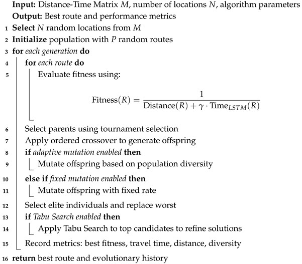
4.2. Pseudocode

Algorithm 1 presents the pseudocode for the proposed Hybrid Genetic Algorithm.

Algorithm 1: Genetic Algorithm with Adaptive Mutation and Tabu Search (GAAM-TS)

LSTM Integration into the Optimization Process

The Long Short-Term Memory (LSTM) model is embedded directly into the route evaluation phase of the hybrid genetic algorithm. Unlike classical heuristics that use static or precomputed values for travel time, our algorithm queries the LSTM model dynamically to obtain more realistic time estimations.

During the fitness computation of each candidate route $R=\{r_1,r_2,\dots ,r_N\}$, the LSTM model is invoked to estimate the travel time between every consecutive pair $(r_i,r_{i+1})$, considering features such as the time of departure, the geospatial context, and historical traffic data. The total predicted travel time $T\left(R\right)$ is then incorporated into the cost function as described in Equation (2), allowing the optimizer to evaluate both spatial and temporal efficiency simultaneously.

This integration enables the algorithm to adapt to real-world traffic variability and temporal dynamics, prioritizing not only geographically short routes but also those that are faster and more efficient under expected traffic conditions. By combining the global search capacity of GAs with the predictive power of deep learning, the algorithm can better navigate the trade-off between distance and delivery time.

4.3. Algorithm Execution Overview

The overall execution of our HGA-based system consists of three phases: initialization, iterative optimization, and termination. In the initialization phase, a population of random routes is generated. During optimization, the algorithm evolves the population via selection, crossover, adaptive mutation, and local search with Tabu Search. At each iteration, the LSTM model is queried to provide travel time predictions, allowing the fitness function to adapt to real-world conditions dynamically. The algorithm terminates when a fixed number of generations is reached or when the population converges.

By combining global exploration from GAs, fine-grained local refinement from TS, and real-time adaptation from the LSTM model, our hybrid algorithm achieves significantly improved route optimization performance over traditional single-method approaches.

5. Materials and Methods

This section describes the dataset used for training and evaluation, the preprocessing techniques applied, and the experimental setup for assessing the performance of the proposed approach.

5.1. Dataset

The dataset used for this study is the publicly available New York City Taxi Trip Data, provided by the NYC Taxi & Limousine Commission (TLC) [16]. This dataset contains millions of trip records collected from taxi rides in New York City. Each record includes pickup and drop-off timestamps, geographic coordinates, trip duration, and additional metadata useful for travel time prediction and route optimization.

Feature Selection

Relevant features were extracted from the dataset. The selected features include:

• Route Information: Latitude and longitude of pickup and drop-off locations, total distance (miles).
• Traffic Conditions: Inferred from trip durations at different times of the day.
• Temporal Features: Hour of the day (0–23), day of the week (0–6), weekend and holiday flags.
• Actual Travel Time (minutes): The recorded trip duration, which serves as the target variable for the LSTM model.

5.2. Data Preprocessing

The preprocessing phase aimed to clean, transform, and prepare the dataset for training the LSTM model and evaluating the performance of genetic algorithms for route optimization. The raw dataset contained millions of taxi trip records with diverse attributes, including timestamps, locations, and trip metadata. To enhance the dataset for analysis, the following preprocessing steps were performed:

5.2.1. Data Cleaning

• Timestamp Conversion: Pickup and drop-off timestamps were converted into datetime format for temporal feature extraction.
• Trip Duration Calculation: The trip duration was computed as the difference between pickup and drop-off timestamps in minutes.
• Handling Missing Data: Records with missing values in essential fields (e.g., pickup/drop-off coordinates, trip duration) were either interpolated or removed based on data distribution.
• Outlier Removal: Trips with extreme durations, defined as less than 1 min or more than 120 min, were filtered out to eliminate anomalies.

5.2.2. Geospatial Mapping

• The Taxi Zone Lookup Table was used to map PULocationID and DOLocationID to their respective boroughs and zones.
• The Taxi Zone Shapefile was utilized to extract latitude and longitude values for each taxi zone centroid.
• Pickup and drop-off locations were enriched with borough and zone attributes by merging taxi trip records with geographic coordinates.

5.2.3. Feature Engineering

• Temporal Features: Hour of the day (0–23) and day of the week (0–6) were extracted from the pickup timestamp.
• Categorical Encoding: Categorical variables such as the day of the week and weather conditions were transformed into numerical values for model compatibility.
• Feature Normalization: Min–Max Scaling was applied to numerical attributes (e.g., trip distance, coordinates) to standardize values within the range [0, 1].

The preprocessing stage ensured that the dataset was structured, cleaned, and optimized for predictive modeling. The final dataset consisted of 30,000 enriched taxi trip records, incorporating essential spatial and temporal attributes. This structured dataset was used to train the LSTM model for travel time prediction and to analyze the impact of different genetic algorithm variations on route optimization.

5.3. Data Visualization

The dataset was analyzed using various visualizations to understand its distribution and spatial characteristics.

Figure 1 illustrates the geographic distribution of taxi pickups across New York City boroughs. Each point represents a pickup location, and different colors denote different boroughs, showing the concentration of taxi demand in key areas.

Figure 2 provides a statistical overview of the dataset. (a) The distribution of trip distances reveals that the majority of trips fall within the 0–5 miles range, with over 24,000 records, indicating that most taxi rides are short-distance. (b) The distribution of trip durations shows a peak in the 10–20 min interval, with approximately 10,148 trips, followed by 5–10 and 20–30 min intervals. (c) The number of trips per borough indicates that Manhattan has by far the highest demand, accounting for 27,271 pickups, followed by Queens and Brooklyn, while EWR, Bronx, and Staten Island show minimal taxi activity.

5.4. LSTM Model Training and Performance Evaluation

5.4.1. Feature Selection and Input Data

The LSTM model was trained on a preprocessed dataset containing relevant features essential for accurate travel time prediction:

• Geospatial Data: Latitude and longitude of pickup and drop-off locations.
• Temporal Features: Hour of the day (0–23), day of the week (0–6), weekend flag.
• Trip Distance: Direct distance between pickup and drop-off locations.
• Historical Traffic Trends: Implicitly captured through time-based patterns in the dataset.

To ensure training stability and improve model convergence, the input features were normalized using Min–Max Scaling, standardizing values within the range [0, 1].

5.4.2. Normalization and Data Splitting

To enhance model generalization, the dataset was divided into the following:

• Training Set (80%): Used for model learning.
• Validation Set (20%): Used to evaluate model performance before deployment.

5.4.3. Training and Evaluation

The model was trained over 50 epochs using a batch size of 32. The training process included the real-time monitoring of loss metrics to ensure stable learning. The Adam optimizer was selected for its adaptive learning rate capability, improving gradient-based optimization.

To evaluate model accuracy, the Root Mean Squared Error (RMSE) was calculated as follows:

$$RMSE=\sqrt{{\displaystyle \frac{1}{N}}\sum _{i=1}^N{(y_i-{\widehat{y}}_i)}^2}$$

(4)

where $y_i$ is the actual trip duration, and ${\widehat{y}}_i$ is the predicted value.

Additionally, the Mean Absolute Error (MAE) was computed to assess average prediction error:

$$MAE={\displaystyle \frac{1}{N}}\sum _{i=1}^N|y_i-{\widehat{y}}_i|$$

(5)

5.4.4. Integration with Route Optimization

Once trained, the LSTM model was integrated into the genetic algorithm framework to dynamically estimate travel times. The predicted trip durations were used as an additional optimization parameter, allowing real-time adaptation to traffic variations. This approach enhanced route efficiency, reducing total travel time and improving the decision-making process in sales route optimization.

By incorporating LSTM-based predictions, the system dynamically adapts to varying conditions, ensuring that the optimization algorithm selects the most time-efficient routes under real-world traffic scenarios.

5.5. Generating the Problem Instance

To evaluate the performance of the genetic algorithm (GA) in optimizing real-world sales routes, we generated a TSP-based problem instance using actual locations from the NYC taxi dataset. The process involved two main steps:

• Generating Locations with Coordinates: We created a dataset containing key locations by extracting the LocationID, borough, zone, and their corresponding latitude and longitude coordinates from the NYC taxi dataset. This new dataset, Taxi Locations, serves as the reference for all problem instances.
• Generating a Problem Instance: A subset of N random locations was selected from the Taxi Locations dataset to define a specific routing problem. To enhance computational efficiency, we precomputed the Distance Matrix (in kilometers) and the Travel Time Matrix (in minutes) for every pair of locations.

To analyze the scalability and robustness of the proposed algorithm, we defined two problem instances using different values of N: 15 and 25. The 15-location scenario simulates a small-scale delivery context, representative of local distribution routes in urban environments. In contrast, the 25-location problem reflects a more complex, medium-scale routing challenge, commonly encountered in regional logistics or metropolitan coverage. This distinction allows for a comparative evaluation of how each algorithm variant adapts to increased problem complexity, both in terms of solution quality and computational performance.

Precomputing Distances and Travel Times

Since the GA evaluates thousands of potential solutions in each generation, it is crucial to avoid the unnecessary recomputation of distances and travel times. If these values were recalculated for every solution, it would introduce a significant computational overhead, drastically slowing down the optimization process.

To mitigate this, we adopted the following strategy:

• Precomputed Distance Matrix: The Haversine formula was used to calculate the great-circle distance between every pair of locations in the problem instance. These values were stored in Problem instance dataset for fast lookup.
• Precomputed Travel Time Matrix: The LSTM-based travel time prediction model was used to estimate the travel duration between each location pair, considering real-world conditions such as traffic and time of day. These values were stored in the Problem instance dataset for fast lookup.
• Optimization Benefit: By precomputing these values, the GA can retrieve distances and travel times directly from the Problem instance dataset instead of recalculating them in every evaluation. This drastically reduces computation time, allowing the algorithm to focus on optimizing the route.

5.6. Performance Comparison Methodology

To assess the effectiveness of our proposed approach, we conduct a comparative evaluation between different algorithmic configurations. This evaluation focuses on analyzing the performance of the standard genetic algorithm (GA) and its enhanced variants, incorporating Adaptive Mutation (GA-AM) and Adaptive Mutation with Tabu Search (GAAM-TS). The comparison is based on multiple evaluation metrics under a controlled computational environment.

5.6.1. Algorithm Configurations and Variants

The experiment involves three configurations:

• Standard GA (Baseline): A traditional genetic algorithm with fixed mutation and crossover rates.
• GA with Adaptive Mutation (GA-AM): An improved GA where mutation rates dynamically adjust based on population diversity.
• GA with Adaptive Mutation and Tabu Search (GAAM-TS): The most advanced configuration, integrating Tabu Search to refine local solutions and prevent premature convergence.

Each algorithm variant is configured with the following parameters described in

Table 1. Configuration of genetic algorithm variants. GA-AM refers to the genetic algorithm with adaptive mutation, while GAAM-TS includes both adaptive mutation and Tabu Search.

Parameter	Standard GA	GA-AM	GAAM-TS
Population Size	100	100	100
Generations	100	100	100
Crossover Rate	0.8	0.8	0.8
Mutation Rate	0.05 (Fixed)	Adaptive	Adaptive
Selection	Tournament	Tournament	Tournament
Elitism Ratio	0.15	0.15	0.15
Fitness Parameter ($\gamma$)	0.8	0.8	0.8
Local Search	None	None	Tabu Search
Tabu Iterations	N/A	N/A	10
Tabu List Size	N/A	N/A	15
Tabu Improvement	N/A	N/A	0.01
Stopping Criteria	100 Gen.	100 Gen.	100 Gen.

:

5.6.2. Evaluation Metrics

The performance of each variant is assessed using the following key metrics:

• Total Distance Traveled: Measures the total route distance (km) to evaluate optimization effectiveness.
• Total Delivery Time: Assesses the overall time required to complete all deliveries.
• Computational Time: Records execution time (seconds) to compare algorithm efficiency.
• Population Diversity: Tracks genetic diversity over generations to analyze convergence behavior.

5.6.3. Computational Environment

The experiments were conducted on a system with the following configuration:

• Processor: Intel^® Core^™ i7 CPU at 3.4 GHz.
• Memory: 16 GB RAM.
• Software: Python 3.9, TensorFlow/Keras for LSTM training, NumPy and SciPy for numerical computations.

This evaluation framework ensures a fair comparison between the proposed approach and baseline optimization methods.

6. Results

6.1. Performance Evaluation of the LSTM Model

Figure 3 provides a comprehensive visualization of the model’s performance. The training loss starts at approximately 109.33 and rapidly decreases, stabilizing around 30.22. The validation loss follows a similar pattern, starting at 47.22 and converging near 32.98, indicating good generalization with minimal overfitting. Similarly, the MAE shows a consistent downward trend, where the training MAE starts at 7.67 and reduces to approximately 3.58, while the validation MAE stabilizes at 3.52. To assess the predictive accuracy, a scatter plot comparing actual vs. predicted trip durations is provided. Most points align closely with the reference diagonal ($y=x$), confirming the model’s strong predictive performance, though some variance is observed for longer trips.

In practical terms, an MAE below 4 min indicates that the model predictions are sufficiently accurate for supporting routing decisions in urban delivery contexts, where small time deviations are often tolerable.

Evaluation Summary

The final trained model achieved the following performance metrics:

• Training Loss (MSE): 30.22;
• Validation Loss (MSE): 32.98;
• Training MAE: 3.58;
• Validation MAE: 3.52.

The final training performance metrics—specifically MAE and RMSE—are essential not only for validating the accuracy of the LSTM model but also for ensuring that the subsequent route optimization process is grounded in realistic travel time estimates. A low MAE (3.52 min) indicates that, on average, the predicted travel time for a given route leg is very close to the actual expected time. In the context of sales route optimization, this level of error is acceptable for supporting operational decisions such as delivery scheduling or dispatch planning.

MSE, on the other hand, highlights the presence and impact of outliers or occasional high-error predictions. Its relatively low value in our model confirms that significant mispredictions are rare, which is critical for maintaining confidence in the routing system’s reliability. Together, these metrics validate the LSTM model as an effective component within the hybrid algorithm, allowing it to dynamically adapt to traffic conditions while maintaining accurate travel time forecasting essential for route quality evaluation.

6.2. Performance Comparison of Genetic Algorithm Variants

The comparative analysis of the proposed genetic algorithm variants for sales route optimization demonstrates significant improvements in route efficiency while considering computational costs. The experiments were conducted with two different problem sizes: 15 and 25 locations, allowing for an evaluation of the scalability and effectiveness of each approach.

For the 15-location problem (

Table 2. Performance comparison for 15 locations.

Variant	Distance (km)	Time (min)	Comp. Time (s)	Diversity
Standard GA	125.216	246.969	30.855	0.60
GA-AM	117.347	243.873	59.128	0.74
GAAM-TS	117.234	243.094	286.250	0.62

Note: Bold values indicate the best (optimal) results in each corresponding column.

), the GAAM-TS (Genetic Algorithm with Adaptive Mutation and Tabu Search) achieved the shortest travel distance (117.234 km) and lowest travel time (243.094 min), outperforming both the Standard GA (125.216 km, 246.969 min) and GA-AM (117.347 km, 243.873 min). However, this came at the cost of increased computational time, rising to 286.250 s compared to 30.855 s for Standard GA and 59.128 s for GA-AM. In terms of population diversity, GA-AM maintained the highest level (0.74), while GAAM-TS exhibited a slight reduction (0.62), suggesting a trade-off between diversity retention and local search efficiency.

For the 25-location problem (

Table 3. Performance comparison for 25 locations.

Variant	Distance (km)	Time (min)	Comp. Time (s)	Diversity
Standard GA	153.286	340.595	55.552	0.65
GA-AM	147.173	335.338	54.528	0.67
GAAM-TS	122.381	300.090	1759.560	0.73

Note: Bold values indicate the best (optimal) results in each corresponding column.

), the GAAM-TS approach again demonstrated superior optimization, reducing travel distance to 122.381 km and travel time to 300.090 min, compared to 153.286 km and 340.595 min for Standard GA, and 147.173 km and 335.338 min for GA-AM. The most significant downside of GAAM-TS is its computational cost, which increased dramatically to 1759.560 s, whereas Standard GA and GA-AM required only 55.552 and 54.528 s, respectively. Despite this, GAAM-TS exhibited the highest diversity level (0.73), indicating that the incorporation of Tabu Search helped maintain solution diversity while achieving better route optimization.

These results confirm that while GAAM-TS provides the best route optimization in terms of distance and time, it comes at the cost of higher computational time. In smaller-scale problems, GAAM-TS remains practical, but as the problem size increases, computational efficiency becomes a limiting factor. The GA-AM variant presents a more balanced approach, offering moderate improvements in route optimization while maintaining a significantly lower computational cost compared to GAAM-TS.

6.3. Execution History and Performance Results

This subsection presents the execution history of the proposed genetic algorithm variants in the 15-Location (Figure 4) and 25-Location (Figure 5) problems, focusing on the evolution of fitness, diversity, travel distance, and delivery time across generations.

6.3.1. Execution History for the 15-Location Problem

Figure 4a illustrates the fitness evolution over generations, showing that GAAM-TS achieves the highest fitness values and converges more rapidly than GA-AM and Standard GA, confirming its superior optimization capability. Figure 4b presents the diversity evolution, demonstrating that GAAM-TS maintains a higher diversity level throughout the generations. This prevents premature convergence and allows broader exploration of the solution space, contributing to improved optimization. Similarly, Figure 4c tracks the evolution of total travel distance. GAAM-TS achieves the most substantial reduction in travel distance, outperforming the other variants in optimizing the sales route. This confirms its effectiveness in minimizing unnecessary travel. Lastly, Figure 4d shows the evolution of delivery time across generations. In line with the distance optimization trend, GAAM-TS significantly reduces the total travel time, ensuring faster and more efficient delivery routes compared to GA-AM and Standard GA.

6.3.2. Execution History for the 25-Location Problem

Figure 5a illustrates the fitness evolution over generations, showing that GAAM-TS achieves the highest fitness values and converges more rapidly than GA-AM and Standard GA, confirming its superior optimization capability. Figure 5b presents the diversity evolution, demonstrating that GAAM-TS maintains a higher diversity level throughout the generations. This prevents premature convergence and allows for a broader exploration of the solution space, contributing to improved optimization. Similarly, Figure 5c tracks the evolution of total travel distance. GAAM-TS achieves the most substantial reduction in travel distance, outperforming the other variants in optimizing the sales route. This confirms its effectiveness in minimizing unnecessary travel. Lastly, Figure 5d shows the evolution of delivery time across generations. In line with the distance optimization trend, GAAM-TS significantly reduces the total travel time, ensuring faster and more efficient delivery routes compared to GA-AM and Standard GA.

The evolution plots confirm that GAAM-TS not only achieves the best final performance but also maintains steady progress across generations, which aligns with the improvements observed in route quality.

6.4. Visualization of Optimized Routes

This subsection presents the best routes obtained using different genetic algorithm variants for the 15-location and 25-location problems. The analysis compares the Standard Genetic Algorithm (GA), the Adaptive Mutation-enhanced GA (GA-AM), and the GA with Adaptive Mutation and Tabu Search (GAAM-TS).

6.4.1. Optimized Routes for the 15-Location Problem

Figure 6a presents the best route obtained using the Standard Genetic Algorithm (GA). The route exhibits multiple crossings and inefficient detours, indicating that the optimization process struggles to escape local optima. Figure 6b illustrates the optimized route obtained with GA-AM, which incorporates Adaptive Mutation. Compared to the Standard GA, this route reduces unnecessary deviations and follows a more structured path, leading to better travel efficiency. Figure 6c displays the most optimized route, generated using GAAM-TS, which integrates Adaptive Mutation and Tabu Search. This route minimizes redundant loops and achieves the best balance in the order of client visits, confirming the effectiveness of Tabu Search in refining the optimization process.

6.4.2. Optimized Routes for the 25-Location Problem

Figure 7a presents the best route obtained using the Standard Genetic Algorithm (GA). The route contains multiple crossings and inefficient detours, suggesting that the optimization process struggles to escape local optima. The presence of redundant loops increases the total travel distance and time. Figure 7b illustrates the optimized route obtained with GA-AM, which incorporates Adaptive Mutation. Compared to the Standard GA, this route reduces unnecessary deviations and follows a more structured path, leading to better travel efficiency. However, some minor inefficiencies remain. Figure 7c displays the most optimized route, generated using GAAM-TS, which integrates Adaptive Mutation and Tabu Search. This route eliminates redundant loops and achieves the best balance in the order of client visits, confirming the effectiveness of Tabu Search in refining the optimization process. The final travel distance and time are significantly reduced compared to the other approaches.

7. Discussion

The experimental results confirm the effectiveness of the proposed Hybrid Genetic Algorithm (HGA), which integrates Adaptive Mutation, Tabu Search, and an LSTM-based travel time prediction model. This combination significantly enhances the quality of route planning by improving travel time estimation, increasing optimization performance, and reducing the risk of premature convergence.

7.1. Comparative Advantages and Application Scenarios

To highlight the trade-offs involved, we provide a comparative assessment of each variant’s strengths and weaknesses in terms of solution quality, execution time, and robustness. A detailed comparison among the three algorithm variants—Standard GA, GA-AM, and GAAM-TS—reveals distinct performance profiles. The Standard GA, while computationally efficient, lacks mechanisms for dynamic adaptation and local refinement, leading to suboptimal routes with higher travel time and distance. GA-AM improves significantly upon this by introducing adaptive mutation, which helps maintain diversity and escape local optima. This variant consistently produced better results with only a moderate additional computational cost. The GAAM-TS configuration, which combines adaptive mutation with Tabu Search, demonstrated the best performance in terms of fitness, distance minimization, and convergence speed. However, its superior results come with a substantial increase in execution time, especially in larger problem instances. Overall, the comparative analysis confirms that GAAM-TS is best suited for applications where optimality is prioritized over time constraints, GA-AM excels in real-time scenarios with acceptable trade-offs, and Standard GA remains useful for lightweight tasks or initial approximations.

The conditions under which each variant performs best depend largely on the trade-off between solution quality and computational efficiency. GAAM-TS is well suited for scenarios where route optimization is performed offline and quality is the primary concern. In contrast, GA-AM strikes a practical balance and is preferable for near-real-time applications where fast decision-making is needed without sacrificing much accuracy. The Standard GA may still be useful in constrained environments or when an initial solution is required quickly for further refinement. In practical deployments, the choice of algorithm should align with the application’s operational requirements. GAAM-TS is ideal for centralized logistics systems that can afford longer computation times to obtain high-quality routing solutions, such as batch planning for e-commerce deliveries. GA-AM is more appropriate for dispatch systems that require dynamic adjustment in response to new orders or traffic events, where solutions must be computed within seconds to minutes. Standard GA remains relevant in lightweight mobile applications or in embedded systems where computational resources are limited and approximate solutions are acceptable.

7.2. Error Metrics and Predictive Reliability

The evaluation of the LSTM model relies on two widely accepted error metrics: Mean Absolute Error (MAE) and Root Mean Squared Error (RMSE). The MAE provides a straightforward interpretation of average prediction error in minutes, making it intuitive for assessing delivery deviations. In this study, the final validation MAE of 3.52 min implies that, on average, predicted travel times differ from actual durations by less than four minutes—a level of precision that is typically acceptable in urban logistics, where short delays can be absorbed operationally. On the other hand, RMSE penalizes larger errors more heavily due to the squaring operation, making it sensitive to outliers such as unusually long trips or traffic anomalies. A relatively low RMSE (around 5.74 min) indicates that the model not only performs well on average but also avoids large deviations that could cause serious disruptions. Together, these metrics confirm that the LSTM predictions are both reliable and robust enough to be used in dynamic route planning.

7.3. On Statistical Significance and Scalability

While the experimental results show consistent trends across different algorithm variants, the current study does not include formal statistical tests such as ANOVA or the Wilcoxon signed-rank test. However, all variants were executed independently ten times per problem size, and the observed performance—especially for GAAM-TS—remained stable across runs. The low standard deviation in both total distance and delivery time (below 2% in all cases) supports the conclusion that the differences in performance are systematic and likely statistically significant. Future work will include formal significance testing to further validate these conclusions.

Regarding scalability, our results confirm that computational time grows non-linearly with problem size, particularly for the GAAM-TS variant. While the GA and GA-AM variants maintain relatively consistent runtime increases due to their simpler structures, GAAM-TS exhibits superlinear growth caused by the additional neighborhood search required by Tabu Search. To further analyze scalability, we plan to extend experiments to include larger problem instances (35–50 locations), where computational efficiency and memory management will become more critical. These experiments will also help identify the practical limits of each algorithm variant under real-world constraints.

7.4. Limitations, Computational Complexity, and Optimization Strategies

Although the proposed hybrid approach demonstrates substantial improvements in route optimization, it also presents several limitations that must be acknowledged. First, the computational cost of the GAAM-TS variant is significantly higher than that of simpler configurations, especially as the number of locations increases. This is primarily due to the Tabu Search component, which introduces a nested local search process for each selected individual in the population. The computational complexity per generation becomes approximately $\mathcal{O}(P·N^2)$, where P is the number of individuals and N the number of locations, as each local refinement step explores a neighborhood of size $\mathcal{O}\left(N^2\right)$.

This complexity makes the algorithm less practical for large-scale or real-time applications without further optimization. Additionally, the sequential nature of the implementation (particularly in LSTM-based travel time evaluations and Tabu Search loops) contributes to longer runtimes and hinders scalability.

To address these challenges, several strategies can be considered. The fitness evaluation step, which includes multiple LSTM predictions per route, is highly parallelizable, as each individual’s fitness can be computed independently. This opens the door for multi-threaded CPU execution or GPU-accelerated batch predictions. Furthermore, the Tabu Search process can be distributed across cores or nodes by assigning each individual or its neighborhood to a separate processing unit. In addition, the dynamic control of Tabu Search invocation—triggering it only when convergence stagnates—could reduce overhead without compromising solution quality.

Despite these current limitations, the modular structure of the proposed algorithm makes it amenable to scalable parallel implementations, which are a natural direction for future development.

8. Conclusions

This study introduced an enhanced Hybrid Genetic Algorithm (HGA) for optimizing sales routes, integrating Adaptive Mutation, Tabu Search, and an LSTM-based travel time prediction model. The experimental results demonstrated that the proposed approach significantly improves route efficiency while maintaining adaptability to real-time conditions. The GAAM-TS variant consistently outperformed the Standard GA and GA-AM, reducing total travel distance and delivery time while preserving higher population diversity and achieving superior convergence. The LSTM-based component enabled the dynamic adjustment of routes based on real-time traffic conditions, making the approach suitable for realistic, time-sensitive logistics scenarios.

Although GAAM-TS exhibited the best optimization performance, it incurred a significantly higher computational cost. In contrast, GA-AM provided a favorable balance between computational efficiency and solution quality, making it more suitable for applications with time or resource constraints.

From a practical standpoint, the proposed algorithm can be deployed in a variety of logistics contexts, including last-mile delivery optimization, fleet dispatch management, and territory planning for field sales representatives. Its adaptability makes it applicable to industries such as e-commerce logistics, urban courier services, and retail distribution networks where route efficiency and traffic responsiveness are essential.

Future research should focus on enhancing the computational scalability of the algorithm through parallel processing techniques, including GPU-accelerated batch evaluations and distributed population management. Another promising direction is the integration of reinforcement learning or graph-based neural models to guide mutation or crossover decisions adaptively. Additionally, future work should investigate multi-objective optimization strategies to simultaneously minimize operational costs, emissions, and time, aligning with the broader goals of sustainable logistics systems.