
Integrated Model Selection and Scalability in Functional Data Analysis Through Bayesian Learning


Abstract
1. Introduction
1.1. Contributions
- Joint selection of optimum latent factors and sparse basis functions: This eliminates constraints on parametric representation dimensionality, avoids information loss from discretization, and extends naturally to higher dimensions or non-Euclidean spaces through nonparametric kernel expansion. It further enhances the interpretability by adaptively choosing the model complexity without testing multiple models separately. We achieve these improvements using a Bayesian paradigm that provides robust and accurate posterior estimates while supporting uncertainty quantification.
- Scalability across domain dimensionality and data size: The proposed method uses VI for faster computation compared to Markov chain Monte Carlo (MCMC) methods, while still being accurate in terms of the estimation of the intrinsic dimensionality and overall covariance structure. BSFDA reduces the overall computation by partitioning the parameters into smaller update groups and introducing a slack variable to further subdivide the weighting matrix (which is part of the kernel structure) into even smaller parts [18], updating fewer blocks at a time and considering all model options. Introducing a slack variable makes the optimization process more efficient by separating different variable groups. This approach scales well with the data size and works efficiently even with large, complex datasets. We demonstrate this on the 4D global oceanic temperature dataset (ARGO), which consists of 127 million data points spanning across the globe for 27 years, with depths of up to 200 m [37].
1.2. Outline
2. Formulation
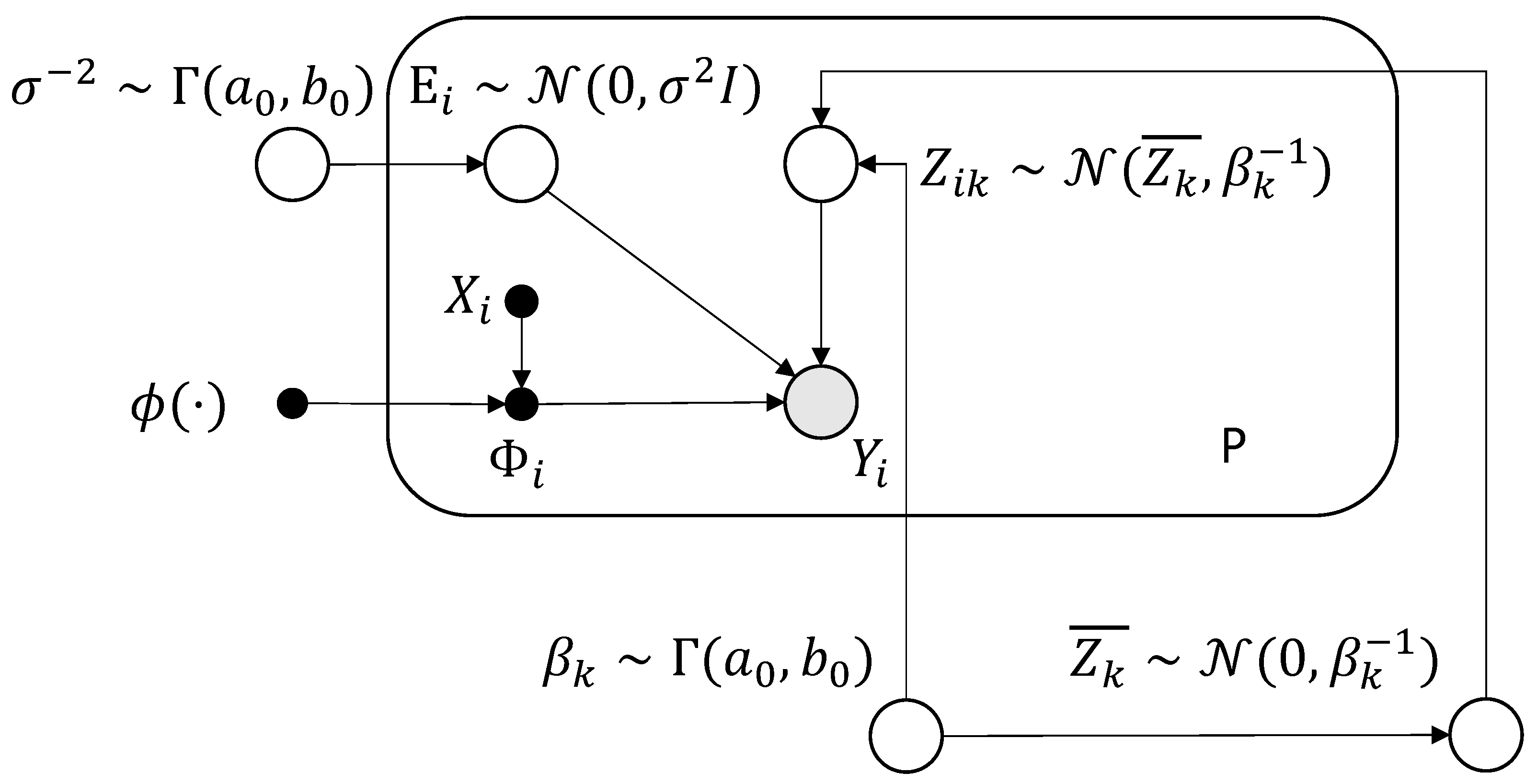
2.1. Generative Model
2.2. Sparse Prior
3. Methods
3.1. Variational Bayesian Inference
Update Steps
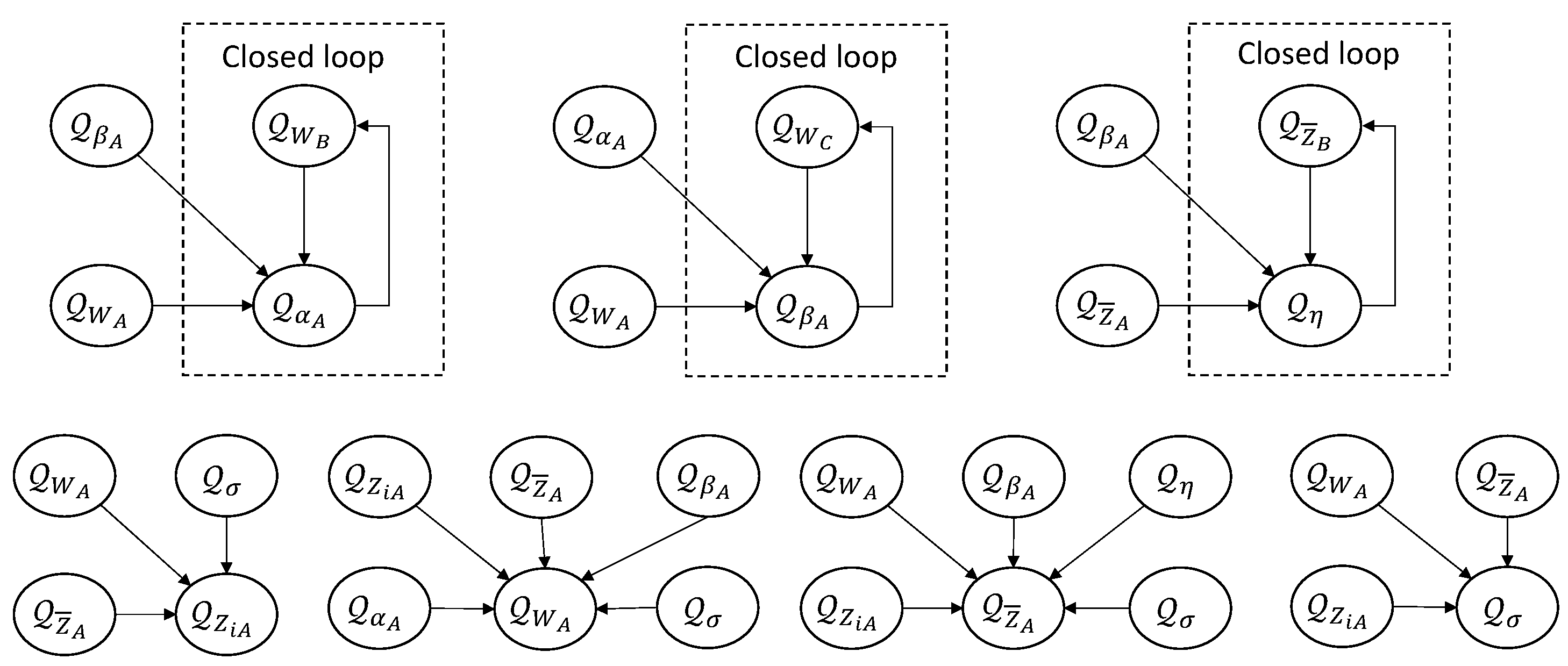
3.2. Scalable Update Strategy
3.2.1. Implicit Factorization
3.2.2. Low-Dimensional Lower Bound
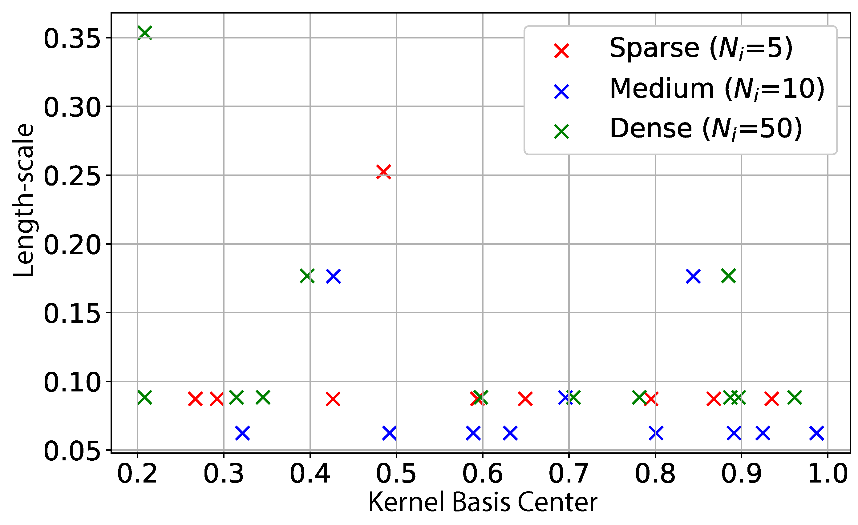
3.2.3. Heuristic for Activation of Basis Functions
| Algorithm 1 Search for new basis functions to activate |
| Sort inactive basis functions by correlation with residuals. Filter through , selecting the most correlated one as . Copy current active surrogate posterior to . Expand dimension in for . Optimize for three iterations using mean field approximation. if expected precision is within threshold then . end if |
4. Faster Variant
5. Results
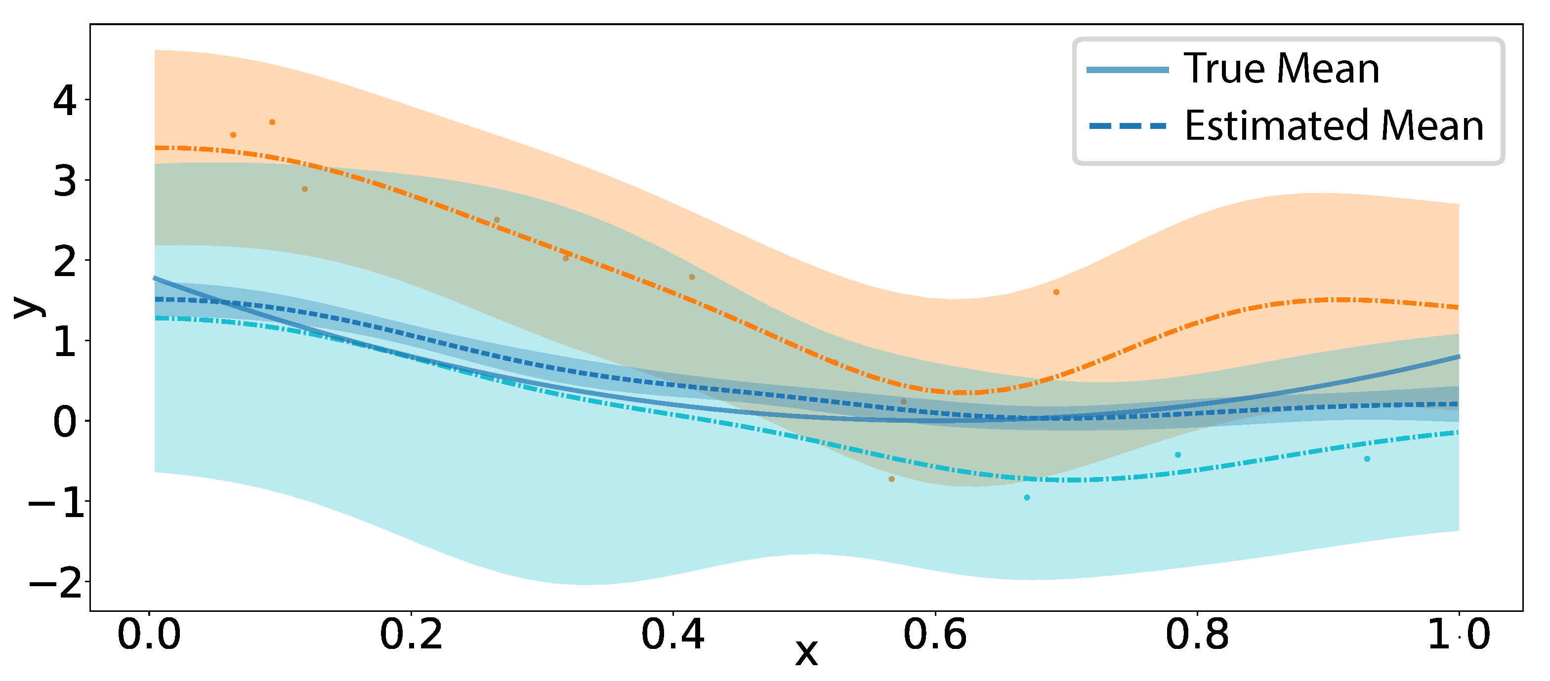
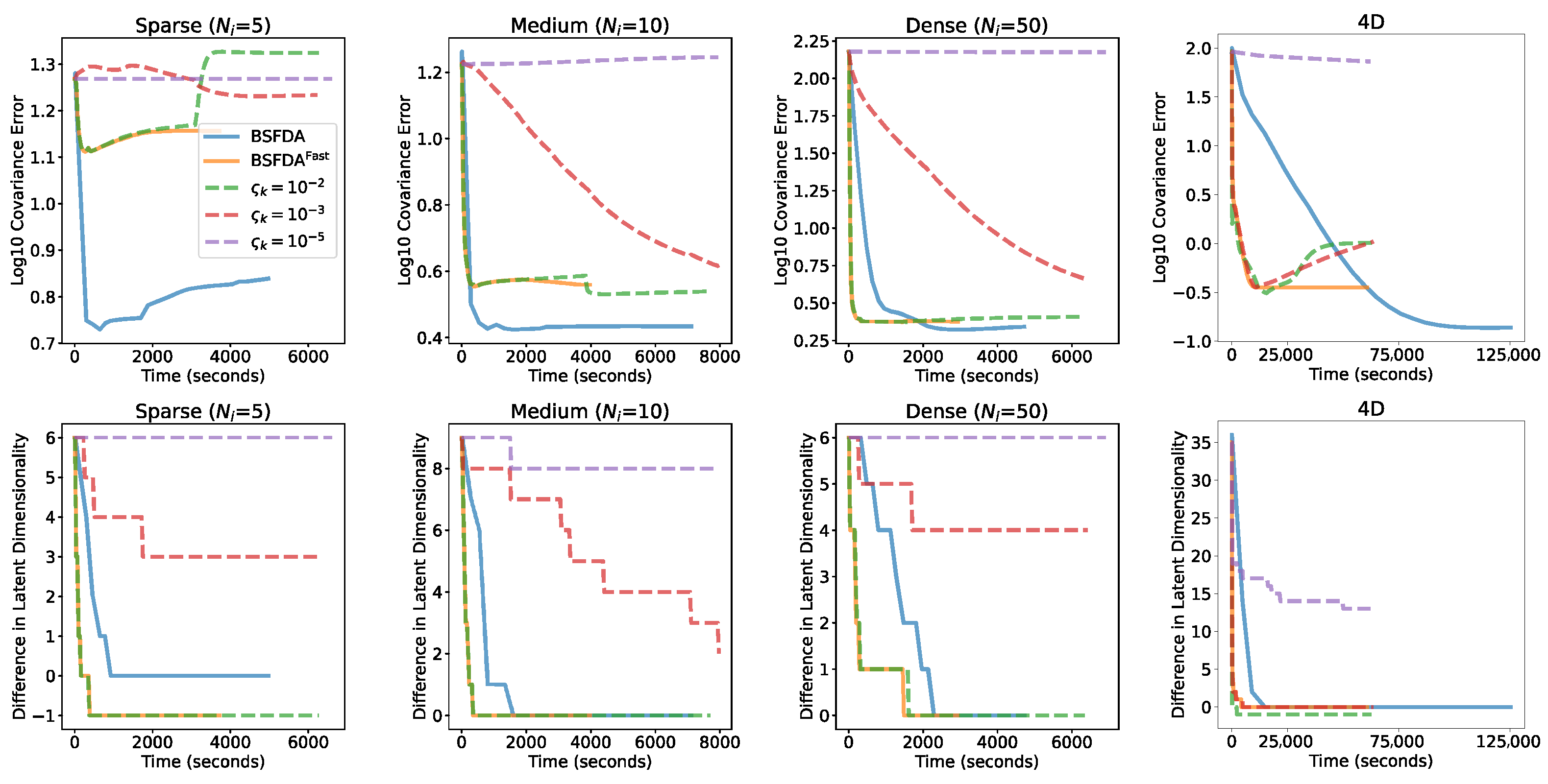
5.1. Simulation Results
5.1.1. Mean Squared Error in Covariance Operator
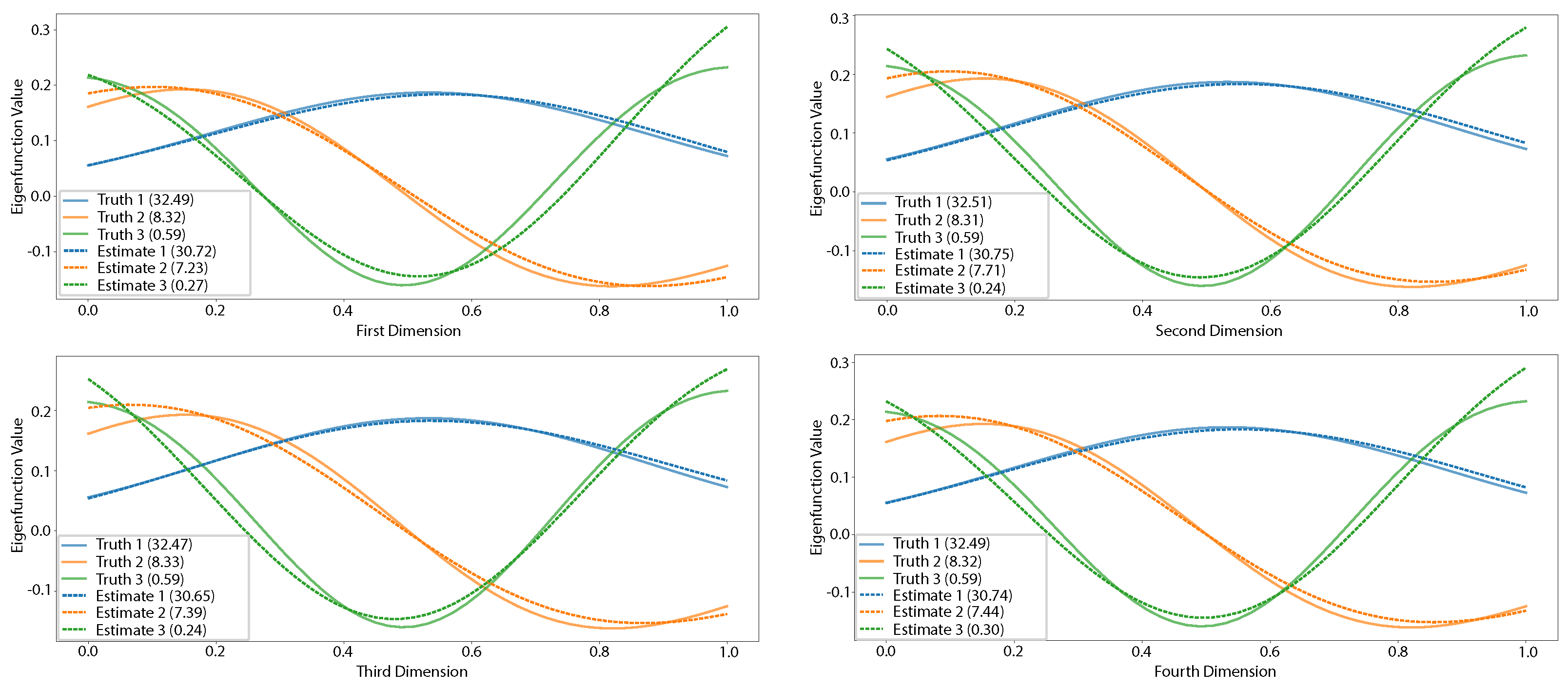
5.1.2. Multidimensional Functional Data Simulation
5.2. Results on Public Datasets
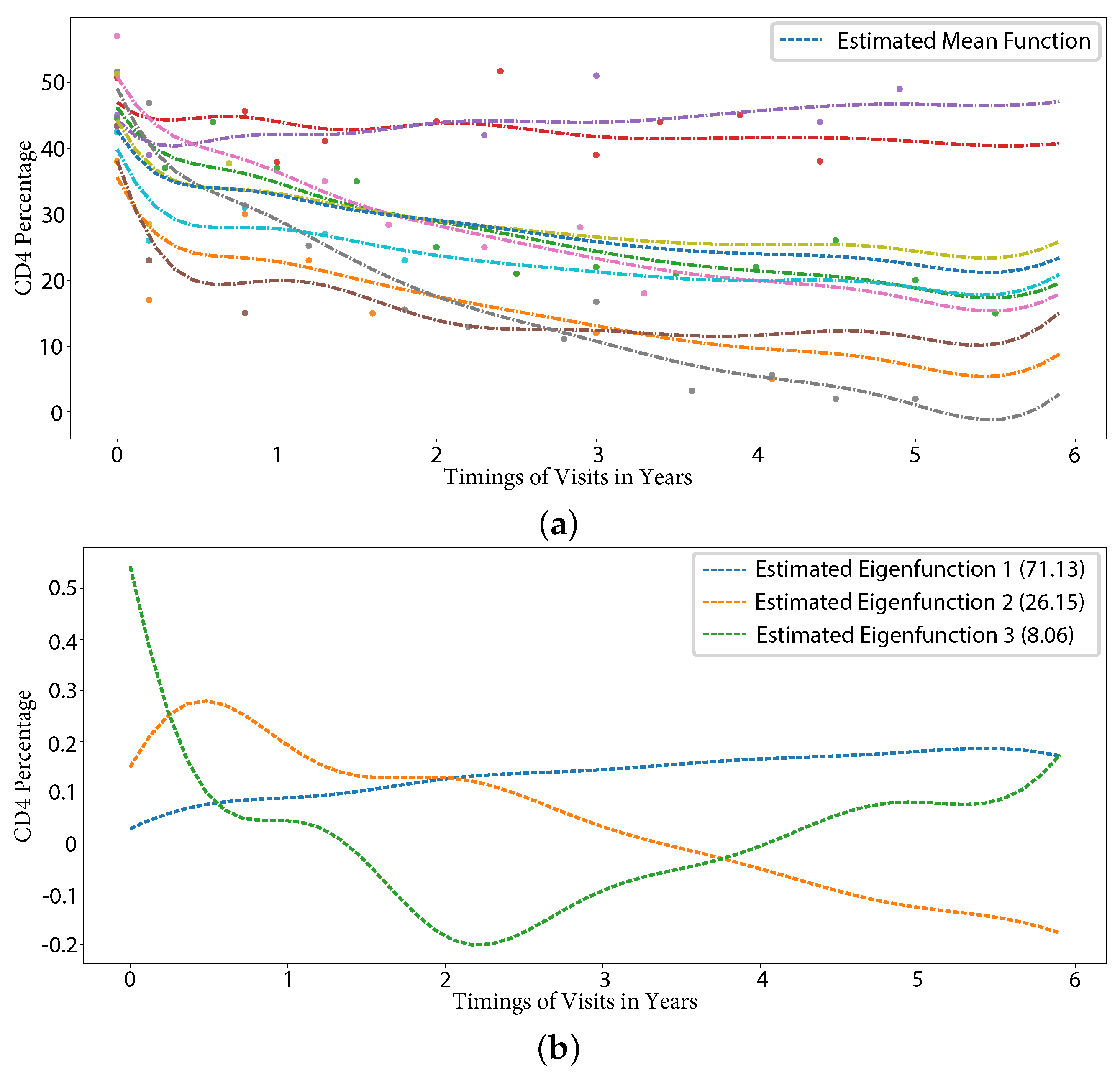
5.2.1. CD4
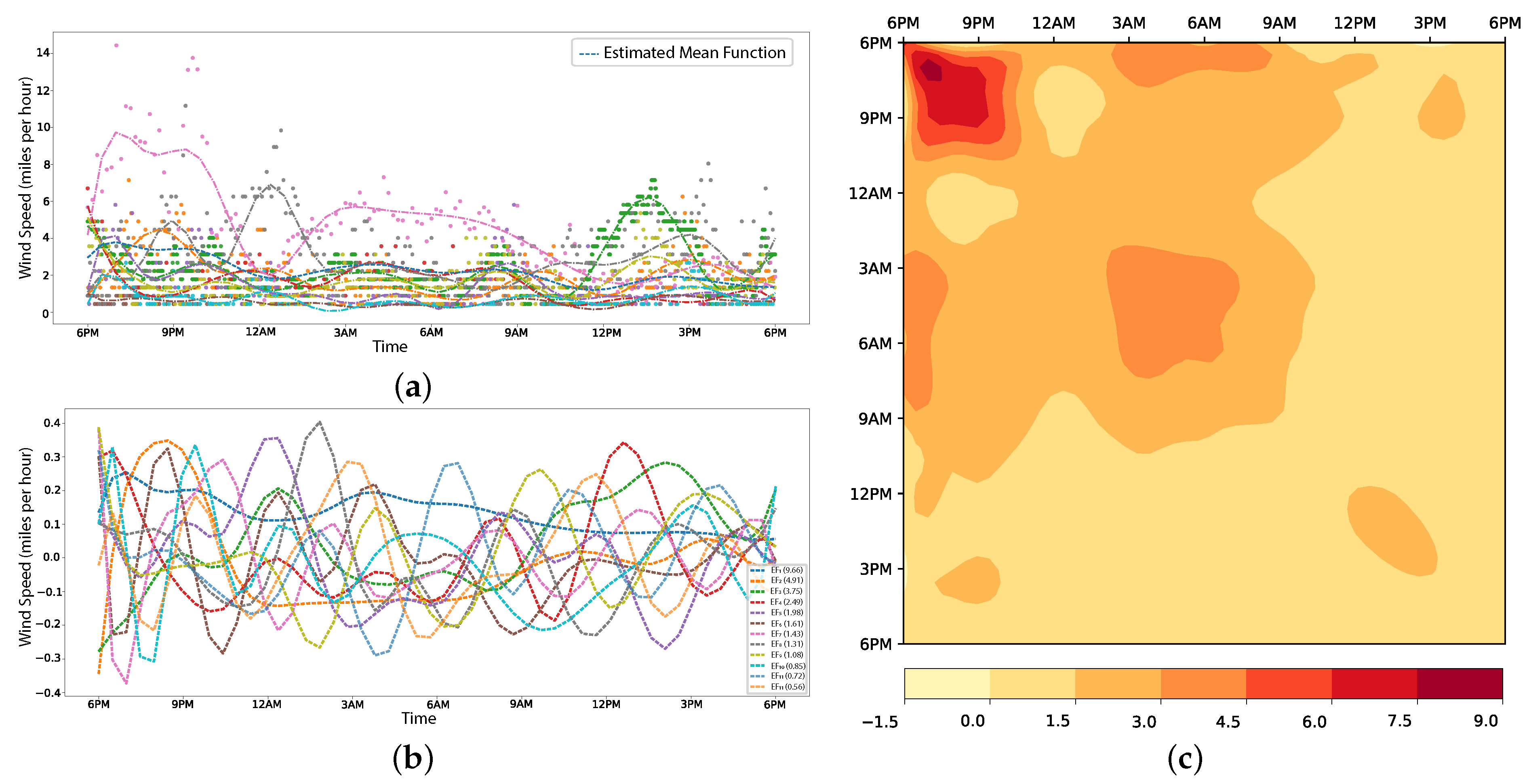
5.2.2. Wind Speed
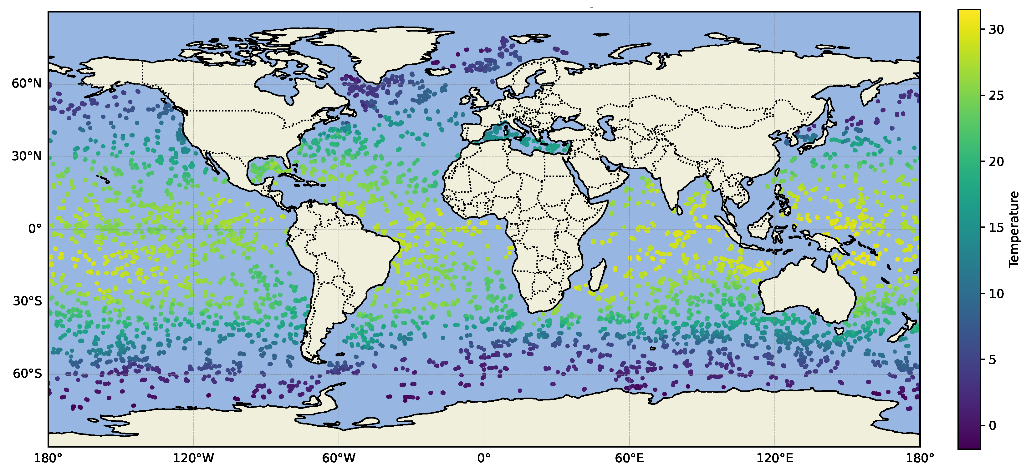
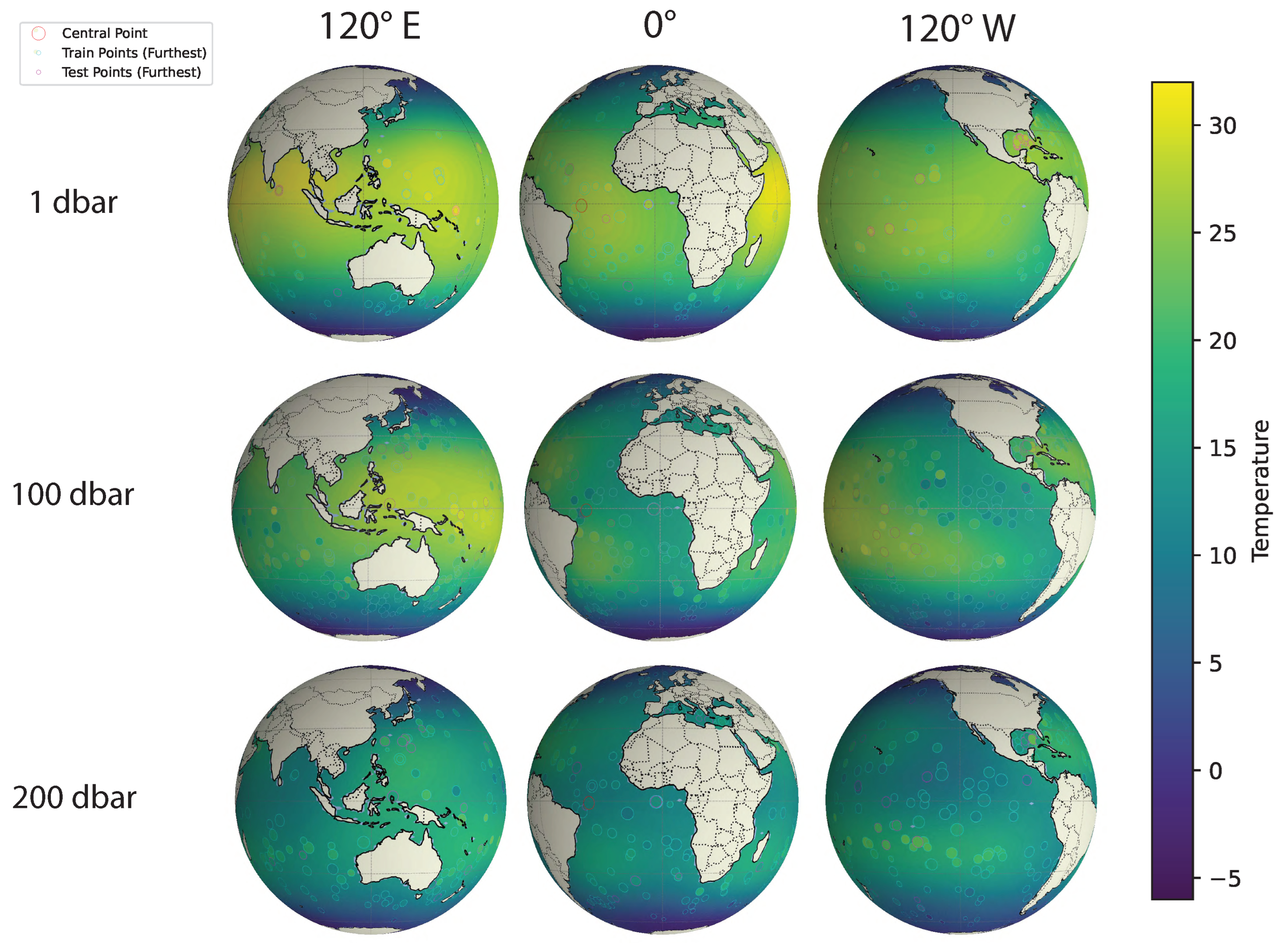
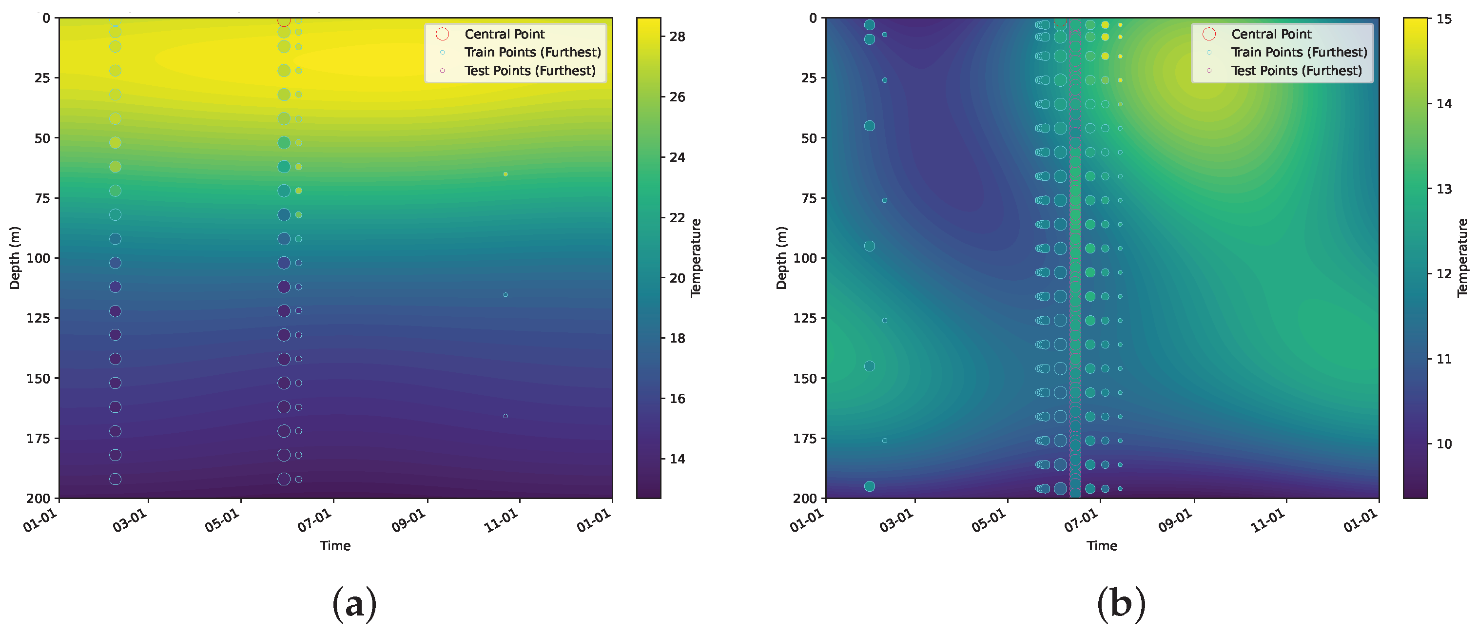
5.2.3. Modeling Large-Scale, Dynamic, Geospatial Data
6. Discussion and Conclusions
Author Contributions
Funding
Data Availability Statement
Conflicts of Interest
Appendix A. System of Notation

| Symbol | Meaning |
|---|---|
| i-th sample function | |
| One M-dimension index | |
| M | Dimension of the index set |
| K | Number of all basis functions |
| J | Number of all components |
| P | Number of sample functions |
| Number of measurements of the i-th sample function | |
| Index set of the i-th sample function | |
| Measurement of the i-th sample function | |
| Component scores of the i-th sample function | |
| Coefficients of basis functions in the mean function | |
| Measurement errors of the i-th sample function | |
| Weighing matrix of basis functions in the eigenfunctions | |
| j-th row and k-th column of W | |
| Kernel function | |
| Scale parameter of (j-th component) | |
| Scale parameter of (k-th basis function) | |
| The standard deviation of measurement errors | |
| The communal scale parameter of | |
| The union of all the centered kernel functions | |
| The value of centered kernel function at | |
| The coefficients of the i-th sample function | |
| The coefficient noise of the i-th sample function | |
| The scale parameter of the k-th coefficient noise |
| Symbol | Meaning |
|---|---|
| All latent variables | |
| The surrogate posterior distribution of variable · | |
| The joint surrogate posterior distribution of all variables except · | |
| The mean and covariance of · in , e.g., | |
| The shape and rate parameters of , e.g., | |
| The expectation of variable · over density | |
| The lower bound of surrogate posterior with K basis functions | |
| The Gram matrix of the kernel functions for the i-th sample function, | |
| The number of active/effective basis functions | |
| The number of active/effective components | |
| The log likelihood of in a multisample relevance vector machine | |
| The covariance of in a multisample relevance vector machine | |
| The posterior covariance of in a multisample relevance vector machine | |
| The log likelihood of in a multisample relevance vector machine | |
| The infinitesimal number | |
| The threshold/tolerance of · |
Appendix B. Variational Update Formulae
Appendix C. Scalable Update for BSFDA
Appendix C.1. Implicit Factorization
Appendix C.2. Scale Parameters
Appendix C.3. Weights and Noise
Appendix C.4. Low-Dimensional Lower Bound
| Algorithm A1 Variational inference |
| Require: ▹Multisample RVM
while True do Update with respect to all parameters using mean field approximation if then ▹Insignificant increase Search for new basis functions using Algorithm 1 if not found then ▹Converged break end if end if Remove dimensions associated with the precision of the maximum values end while Get rid of dimensions associated with and |
Appendix D. Scalable Update for BSFDAFast
Appendix E. Fast Initialization
Appendix E.1. Maximum Likelihood Estimation
| Algorithm A2 Multisample relevance vector machine |
| while is not converged
do ▹ ▹ Sparsity factor. ▹Quality factor. if then ▹Precision is finite else ▹Precision is infinite and the dimension is removed end if ▹ ▹ end while |
Appendix E.2. Optimization of β,
Appendix E.3. Optimization of σ
Appendix F. Experiments
Appendix F.1. Benchmark Simulation
| AIC | BIC | fpca | BSFDA | ||||||||
|---|---|---|---|---|---|---|---|---|---|---|---|
| 5 | ≤1 | 0.000 | 0.000 | 0.155 | 0.005 | 0.000 | 0.000 | 0.000 | 0.000 | 0.000 | 0.000 |
| =2 | 0.008 | 0.405 | 0.335 | 0.565 | 0.215 | 0.000 | 0.000 | 0.000 | 0.000 | 0.985 | |
| =3 | 0.000 | 0.580 | 0.380 | 0.410 | 0.735 | 0.650 | 0.880 | 0.645 | 0.995 | 0.015 | |
| =4 | 0.121 | 0.010 | 0.115 | 0.010 | 0.045 | 0.335 | 0.120 | 0.235 | 0.005 | 0.000 | |
| ≥5 | 0.870 | 0.005 | 0.015 | 0.010 | 0.005 | 0.015 | 0.000 | 0.120 | 0.000 | 0.000 | |
| 10 | ≤1 | 0.000 | 0.000 | 0.000 | 0.000 | 0.000 | 0.000 | 0.000 | 0.000 | 0.000 | 0.000 |
| =2 | 0.000 | 0.005 | 0.040 | 0.040 | 0.005 | 0.000 | 0.000 | 0.000 | 0.000 | 0.075 | |
| =3 | 0.000 | 0.980 | 0.670 | 0.955 | 0.985 | 0.880 | 0.920 | 0.645 | 1.000 | 0.910 | |
| =4 | 0.000 | 0.015 | 0.255 | 0.000 | 0.010 | 0.120 | 0.080 | 0.235 | 0.000 | 0.015 | |
| ≥5 | 1.000 | 0.000 | 0.035 | 0.005 | 0.000 | 0.000 | 0.000 | 0.120 | 0.000 | 0.000 | |
| 50 | ≤1 | 0.000 | 0.000 | 0.000 | 0.000 | 0.000 | 0.000 | 0.000 | 0.000 | 0.000 | 0.000 |
| =2 | 0.000 | 0.000 | 0.000 | 0.000 | 0.000 | 0.000 | 0.000 | 0.000 | 0.000 | 0.000 | |
| =3 | 0.000 | 1.000 | 0.830 | 1.000 | 1.000 | 1.000 | 1.000 | 0.890 | 0.980 | 0.945 | |
| =4 | 0.000 | 0.000 | 0.150 | 0.000 | 0.000 | 0.000 | 0.000 | 0.060 | 0.020 | 0.050 | |
| ≥5 | 1.000 | 0.000 | 0.020 | 0.000 | 0.000 | 0.000 | 0.000 | 0.050 | 0.000 | 0.005 |
| AIC | BIC | fpca | BSFDA | ||||||||
|---|---|---|---|---|---|---|---|---|---|---|---|
| 5 | ≤1 | 0.000 | 0.000 | 0.230 | 0.000 | 0.000 | 0.000 | 0.000 | 0.000 | 0.000 | 0.000 |
| =2 | 0.000 | 0.205 | 0.395 | 0.000 | 0.140 | 0.050 | 0.075 | 0.000 | 0.000 | 0.960 | |
| =3 | 0.005 | 0.630 | 0.245 | 0.375 | 0.605 | 0.570 | 0.620 | 0.475 | 1.000 | 0.040 | |
| =4 | 0.125 | 0.155 | 0.110 | 0.440 | 0.210 | 0.345 | 0.275 | 0.350 | 0.000 | 0.000 | |
| ≥5 | 0.870 | 0.010 | 0.020 | 0.185 | 0.045 | 0.035 | 0.030 | 0.175 | 0.000 | 0.000 | |
| 10 | ≤1 | 0.000 | 0.000 | 0.000 | 0.000 | 0.000 | 0.000 | 0.000 | 0.000 | 0.000 | 0.000 |
| =2 | 0.000 | 0.000 | 0.170 | 0.000 | 0.000 | 0.000 | 0.000 | 0.000 | 0.000 | 0.000 | |
| =3 | 0.000 | 0.710 | 0.665 | 0.570 | 0.805 | 0.825 | 0.850 | 0.640 | 1.000 | 0.995 | |
| =4 | 0.005 | 0.260 | 0.135 | 0.355 | 0.185 | 0.175 | 0.150 | 0.235 | 0.000 | 0.005 | |
| ≥5 | 0.995 | 0.030 | 0.030 | 0.075 | 0.010 | 0.000 | 0.000 | 0.125 | 0.000 | 0.000 | |
| 50 | ≤1 | 0.000 | 0.000 | 0.000 | 0.000 | 0.000 | 0.000 | 0.000 | 0.000 | 0.000 | 0.000 |
| =2 | 0.000 | 0.000 | 0.000 | 0.000 | 0.000 | 0.000 | 0.000 | 0.000 | 0.000 | 0.000 | |
| =3 | 0.000 | 0.630 | 0.795 | 0.955 | 0.945 | 1.000 | 1.000 | 0.950 | 1.000 | 0.950 | |
| =4 | 0.000 | 0.320 | 0.185 | 0.045 | 0.055 | 0.000 | 0.000 | 0.020 | 0.000 | 0.050 | |
| ≥5 | 1.000 | 0.050 | 0.020 | 0.000 | 0.000 | 0.000 | 0.000 | 0.030 | 0.000 | 0.000 |
| AIC | BIC | fpca | BSFDA | ||||||||
|---|---|---|---|---|---|---|---|---|---|---|---|
| 5 | ≤1 | 0.000 | 0.000 | 0.335 | 0.000 | 0.000 | 0.000 | 0.000 | 0.000 | 0.000 | 0.000 |
| =2 | 0.025 | 0.035 | 0.260 | 0.220 | 0.005 | 0.000 | 0.005 | 0.000 | 0.000 | 0.025 | |
| =3 | 0.005 | 0.720 | 0.325 | 0.640 | 0.590 | 0.320 | 0.400 | 0.450 | 0.995 | 0.945 | |
| =4 | 0.130 | 0.170 | 0.080 | 0.075 | 0.280 | 0.640 | 0.565 | 0.360 | 0.005 | 0.030 | |
| ≥5 | 0.840 | 0.075 | 0.000 | 0.065 | 0.125 | 0.030 | 0.030 | 0.190 | 0.000 | 0.000 | |
| 10 | ≤1 | 0.000 | 0.000 | 0.005 | 0.000 | 0.000 | 0.000 | 0.000 | 0.000 | 0.000 | 0.000 |
| =2 | 0.015 | 0.000 | 0.035 | 0.000 | 0.000 | 0.000 | 0.000 | 0.000 | 0.000 | 0.000 | |
| =3 | 0.000 | 0.580 | 0.770 | 0.965 | 0.665 | 0.740 | 0.755 | 0.440 | 0.995 | 1.000 | |
| =4 | 0.000 | 0.400 | 0.145 | 0.030 | 0.320 | 0.260 | 0.245 | 0.380 | 0.005 | 0.000 | |
| ≥5 | 0.985 | 0.020 | 0.045 | 0.005 | 0.015 | 0.000 | 0.000 | 0.180 | 0.000 | 0.000 | |
| 50 | ≤1 | 0.000 | 0.000 | 0.000 | 0.000 | 0.000 | 0.000 | 0.000 | 0.000 | 0.000 | 0.000 |
| =2 | 0.000 | 0.000 | 0.000 | 0.000 | 0.000 | 0.000 | 0.000 | 0.000 | 0.015 | 0.000 | |
| =3 | 0.000 | 1.000 | 0.775 | 1.000 | 1.000 | 1.000 | 1.000 | 0.765 | 0.980 | 0.920 | |
| =4 | 0.000 | 0.000 | 0.200 | 0.000 | 0.000 | 0.000 | 0.000 | 0.110 | 0.005 | 0.050 | |
| ≥5 | 1.000 | 0.000 | 0.025 | 0.000 | 0.000 | 0.000 | 0.000 | 0.125 | 0.000 | 0.030 |
| AIC | BIC | fpca | BSFDA | ||||||||
|---|---|---|---|---|---|---|---|---|---|---|---|
| 5 | ≤1 | 0.000 | 0.000 | 0.315 | 0.000 | 0.000 | 0.000 | 0.000 | 0.000 | 0.000 | 0.000 |
| =2 | 0.015 | 0.020 | 0.180 | 0.160 | 0.015 | 0.000 | 0.000 | 0.000 | 0.000 | 0.000 | |
| =3 | 0.015 | 0.710 | 0.410 | 0.640 | 0.560 | 0.515 | 0.575 | 0.370 | 1.000 | 0.975 | |
| =4 | 0.145 | 0.185 | 0.070 | 0.095 | 0.260 | 0.450 | 0.390 | 0.515 | 0.000 | 0.025 | |
| ≥5 | 0.825 | 0.085 | 0.025 | 0.105 | 0.165 | 0.035 | 0.035 | 0.115 | 0.000 | 0.000 | |
| 10 | ≤1 | 0.000 | 0.000 | 0.010 | 0.000 | 0.000 | 0.000 | 0.000 | 0.000 | 0.000 | 0.000 |
| =2 | 0.000 | 0.000 | 0.005 | 0.000 | 0.000 | 0.000 | 0.000 | 0.000 | 0.000 | 0.000 | |
| =3 | 0.000 | 0.830 | 0.775 | 0.920 | 0.900 | 0.750 | 0.760 | 0.350 | 0.995 | 0.990 | |
| =4 | 0.000 | 0.150 | 0.190 | 0.045 | 0.085 | 0.250 | 0.240 | 0.380 | 0.005 | 0.010 | |
| ≥5 | 1.000 | 0.020 | 0.020 | 0.035 | 0.015 | 0.000 | 0.000 | 0.270 | 0.000 | 0.000 | |
| 50 | ≤1 | 0.000 | 0.000 | 0.000 | 0.000 | 0.000 | 0.000 | 0.000 | 0.000 | 0.000 | 0.000 |
| =2 | 0.000 | 0.000 | 0.000 | 0.000 | 0.000 | 0.000 | 0.000 | 0.000 | 0.010 | 0.000 | |
| =3 | 0.000 | 0.945 | 0.835 | 1.000 | 1.000 | 1.000 | 1.000 | 0.730 | 0.950 | 0.935 | |
| =4 | 0.000 | 0.055 | 0.140 | 0.000 | 0.000 | 0.000 | 0.000 | 0.160 | 0.040 | 0.055 | |
| ≥5 | 1.000 | 0.000 | 0.025 | 0.000 | 0.000 | 0.000 | 0.000 | 0.110 | 0.000 | 0.010 |
| AIC | BIC | fpca | BSFDA | ||||||||
|---|---|---|---|---|---|---|---|---|---|---|---|
| 5 | ≤4 | 0.005 | 0.165 | 0.835 | 0.580 | 0.060 | 0.000 | 0.000 | 0.010 | 0.000 | 0.060 |
| =5 | 0.005 | 0.330 | 0.020 | 0.345 | 0.335 | 0.575 | 0.590 | 0.010 | 0.075 | 0.515 | |
| =6 | 0.705 | 0.470 | 0.090 | 0.070 | 0.545 | 0.425 | 0.410 | 0.855 | 0.925 | 0.160 | |
| =7 | 0.245 | 0.035 | 0.050 | 0.005 | 0.060 | 0.000 | 0.000 | 0.115 | 0.000 | 0.160 | |
| ≥8 | 0.040 | 0.000 | 0.005 | 0.000 | 0.000 | 0.000 | 0.000 | 0.010 | 0.000 | 0.105 | |
| 10 | ≤4 | 0.005 | 0.000 | 0.000 | 0.000 | 0.000 | 0.000 | 0.000 | 0.000 | 0.000 | 0.000 |
| =5 | 0.000 | 0.000 | 0.030 | 0.145 | 0.000 | 0.425 | 0.425 | 0.000 | 0.000 | 0.000 | |
| =6 | 0.065 | 0.570 | 0.525 | 0.775 | 0.705 | 0.575 | 0.575 | 0.500 | 1.000 | 0.930 | |
| =7 | 0.475 | 0.280 | 0.165 | 0.020 | 0.185 | 0.000 | 0.000 | 0.405 | 0.000 | 0.035 | |
| 0.455 | 0.150 | 0.030 | 0.060 | 0.110 | 0.000 | 0.000 | 0.095 | 0.000 | 0.035 | ||
| 50 | ≤4 | 0.000 | 0.000 | 0.005 | 0.000 | 0.000 | 0.000 | 0.000 | 0.000 | 0.000 | 0.000 |
| =5 | 0.065 | 0.000 | 0.000 | 0.000 | 0.000 | 0.130 | 0.130 | 0.005 | 0.000 | 0.000 | |
| =6 | 0.000 | 0.260 | 0.590 | 0.980 | 0.965 | 0.870 | 0.770 | 0.695 | 0.995 | 0.925 | |
| =7 | 0.000 | 0.405 | 0.325 | 0.010 | 0.035 | 0.000 | 0.000 | 0.250 | 0.005 | 0.045 | |
| ≥8 | 0.935 | 0.335 | 0.080 | 0.010 | 0.000 | 0.000 | 0.000 | 0.050 | 0.000 | 0.030 |
Appendix F.1.1. Performance of LFRM
- Gamma prior for white noise and correlated noise;
- Length scale;
- Number of basis functions;
- Number of iterations.
- Standard LFRM estimated 10–14 components;
- LFRM with 10 length scales estimated 6–8 components;
- LFRM with a low-correlated-noise prior estimated 8–15 components;
- LFRM with a noninformative-like correlated-noise prior estimated 10–14 components.
- Correlated noise interference: The correlated noise can obscure the true signal.
- Prior specification: LFRM’s precision parameter priors are potentially less noninformative and not as sparse as those sparse Bayesian learning priors [30] in BSFDA.
- Element-wise vs. column-wise precision: The element-wise precision parameters in LFRM might compensate in a way that reduces the overall sparsity.
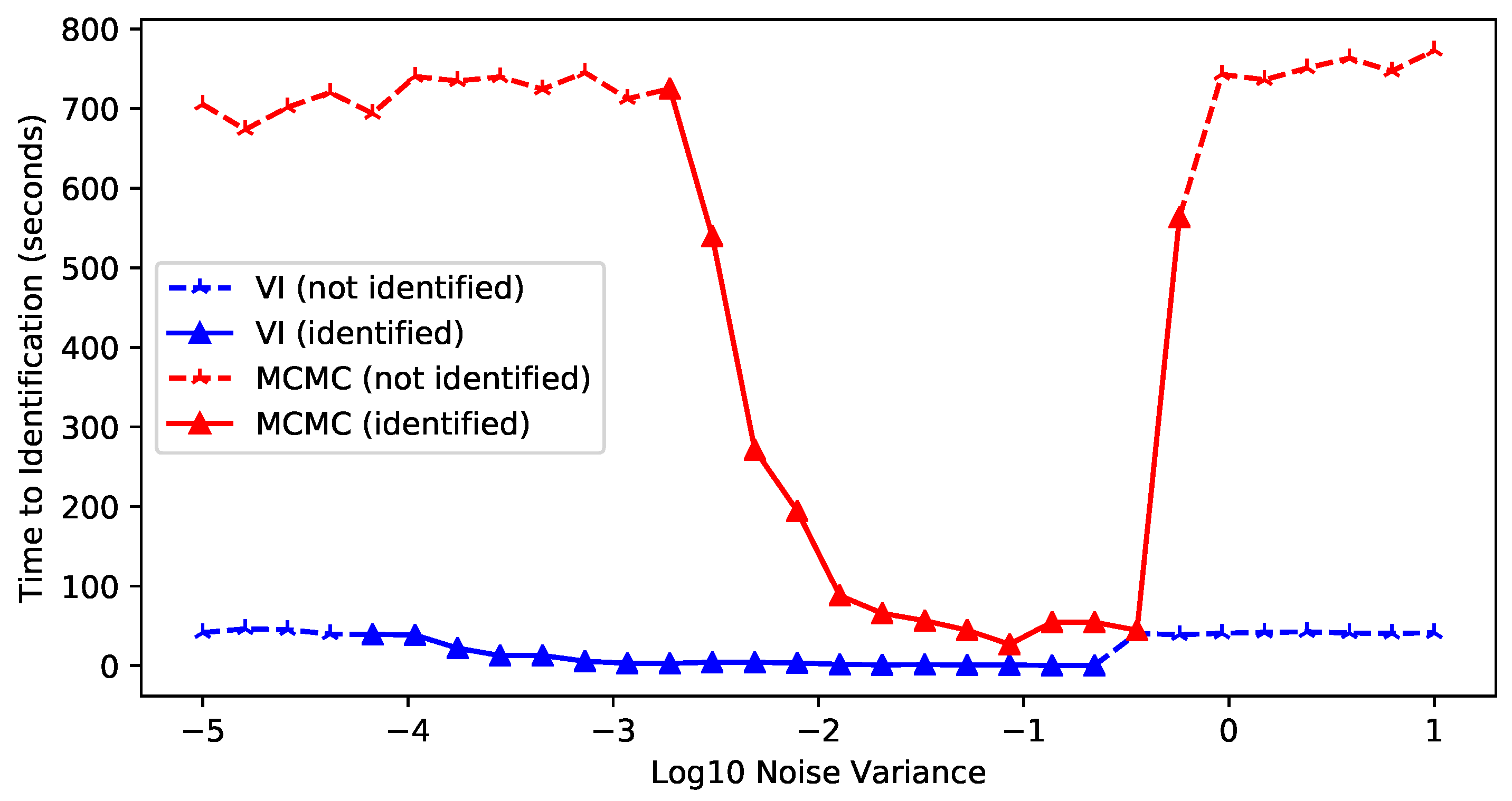
Appendix F.2. Variational Inference vs. MCMC
- When the noise level was close to the signal, neither MCMC or VI found the true dimension in the limited iterations (and probably never would have), because the data were heavily polluted.
- As the noise level decreased toward zero, the number of iterations (and runtime) required for satisfactory estimation increased dramatically; VI began to fail around a noise level of and MCMC sampling around , within the set time constraints.
- Across the 10 noise levels (about to ) where both successfully identified the correct dimensionality, VI was consistently completed much faster than MCMC sampling. VI was 85.57 ± 50.24 times faster on average, in the range of 32.46 to 189.12.
References
- Wang, J.L.; Chiou, J.M.; Müller, H.G. Functional Data Analysis. Annu. Rev. Stat. Its Appl. 2016, 3, 257–295. [Google Scholar] [CrossRef]
- Ramsay, J.O.; Silverman, B.W. Applied Functional Data Analysis: Methods and Case Studies; Springer: Berlin/Heidelberg, Germany, 2002. [Google Scholar]
- Rice, J.A.; Silverman, B.W. Estimating the Mean and Covariance Structure Nonparametrically When the Data are Curves. J. R. Stat. Soc. Ser. B Stat. Methodol. 1991, 53, 233–243. [Google Scholar] [CrossRef]
- Aneiros, G.; Cao, R.; Fraiman, R.; Genest, C.; Vieu, P. Recent advances in functional data analysis and high-dimensional statistics. J. Multivar. Anal. 2019, 170, 3–9. [Google Scholar] [CrossRef]
- Li, Y.; Qiu, Y.; Xu, Y. From multivariate to functional data analysis: Fundamentals, recent developments, and emerging areas. J. Multivar. Anal. 2022, 188, 104806. [Google Scholar] [CrossRef]
- Happ, C.; Greven, S. Multivariate Functional Principal Component Analysis for Data Observed on Different (Dimensional) Domains. J. Am. Stat. Assoc. 2018, 113, 649–659. [Google Scholar] [CrossRef]
- Kowal, D.R.; Canale, A. Semiparametric Functional Factor Models with Bayesian Rank Selection. Bayesian Anal. 2023, 18, 1161–1189. [Google Scholar] [CrossRef]
- Suarez, A.J.; Ghosal, S. Bayesian Estimation of Principal Components for Functional Data. Bayesian Anal. 2017, 12, 311–333. [Google Scholar] [CrossRef]
- Sun, T.Y.; Kowal, D.R. Ultra-Efficient MCMC for Bayesian Longitudinal Functional Data Analysis. J. Comput. Graph. Stat. 2024, 34, 34–46. [Google Scholar] [CrossRef]
- Rasmussen, C.E.; Williams, C.K.I. Gaussian Processes for Machine Learning; Adaptive Computation and Machine Learning; MIT Press: Cambridge, MA. USA, 2006; p. 248. [Google Scholar]
- Yao, F.; Müller, H.G.; Wang, J.L. Functional Data Analysis for Sparse Longitudinal Data. J. Am. Stat. Assoc. 2005, 100, 577–590. [Google Scholar] [CrossRef]
- Di, C.Z.; Crainiceanu, C.M.; Caffo, B.S.; Punjabi, N.M. Multilevel functional principal component analysis. Ann. Appl. Stat. 2009, 3, 458–488. [Google Scholar] [CrossRef]
- Peng, J.; Paul, D. A geometric approach to maximum likelihood estimation of the functional principal components from sparse longitudinal data. J. Comput. Graph. Stat. 2009, 18, 995–1015. [Google Scholar] [CrossRef]
- Chiou, J.M.; Yang, Y.F.; Chen, Y.T. Multivariate functional principal component analysis: A normalization approach. Stat. Sin. 2014, 24, 1571–1596. [Google Scholar] [CrossRef]
- Trefethen, L.N. Approximation Theory and Approximation Practice, Extended Edition; SIAM: Philadelphia, PA, USA, 2019. [Google Scholar]
- Bungartz, H.J.; Griebel, M. Sparse grids. Acta Numer. 2004, 13, 147–269. [Google Scholar] [CrossRef]
- Shi, H.; Yang, Y.; Wang, L.; Ma, D.; Beg, M.F.; Pei, J.; Cao, J. Two-Dimensional Functional Principal Component Analysis for Image Feature Extraction. J. Comput. Graph. Stat. 2022, 31, 1127–1140. [Google Scholar] [CrossRef]
- Montagna, S.; Tokdar, S.T.; Neelon, B.; Dunson, D.B. Bayesian Latent Factor Regression for Functional and Longitudinal Data. Biometrics 2012, 68, 1064–1073. [Google Scholar] [CrossRef]
- Kowal, D.R.; Bourgeois, D.C. Bayesian Function-on-Scalars Regression for High-Dimensional Data. J. Comput. Graph. Stat. 2020, 29, 629–638. [Google Scholar] [CrossRef]
- Sousa, P.H.T.O.; Souza, C.P.E.d.; Dias, R. Bayesian adaptive selection of basis functions for functional data representation. J. Appl. Stat. 2024, 51, 958–992. [Google Scholar] [CrossRef]
- Li, Y.; Wang, N.; Carroll, R.J. Selecting the Number of Principal Components in Functional Data. J. Am. Stat. Assoc. 2013, 108, 1284–1294. [Google Scholar] [CrossRef]
- Shamshoian, J.; Şentürk, D.; Jeste, S.; Telesca, D. Bayesian analysis of longitudinal and multidimensional functional data. Biostatistics 2022, 23, 558–573. [Google Scholar] [CrossRef]
- Huo, S.; Morris, J.S.; Zhu, H. Ultra-Fast Approximate Inference Using Variational Functional Mixed Models. J. Comput. Graph. Stat. 2023, 32, 353–365. [Google Scholar] [CrossRef]
- Liu, Y.; Qiao, X.; Pei, Y.; Wang, L. Deep Functional Factor Models: Forecasting High-Dimensional Functional Time Series via Bayesian Nonparametric Factorization. In Proceedings of the International Conference on Machine Learning, PMLR, Vienna, Austria, 21–27 July 2024; pp. 31709–31727. [Google Scholar]
- Jolliffe, I.T.; Cadima, J. Principal component analysis: A review and recent developments. Philos. Trans. R. Soc. Math. Phys. Eng. Sci. 2016, 374, 20150202. [Google Scholar] [CrossRef] [PubMed]
- Tipping, M.E.; Bishop, C.M. Probabilistic principal component analysis. J. R. Stat. Soc. Ser. B Stat. Methodol. 1999, 61, 611–622. [Google Scholar] [CrossRef]
- Ilin, A.; Raiko, T. Practical approaches to principal component analysis in the presence of missing values. J. Mach. Learn. Res. 2010, 11, 1957–2000. [Google Scholar]
- Bishop, C.M. Variational Principal Components. In Proceedings of the Ninth International Conference on Artificial Neural Networks, ICANN’99, Edinburgh, UK, 7–10 September 1999; IEEE: Piscataway, NJ, USA, 1999; pp. 509–514. [Google Scholar]
- Tipping, M.E.; Bishop, C.M. Mixtures of probabilistic principal component analyzers. Neural Comput. 1999, 11, 443–482. [Google Scholar] [CrossRef]
- Tipping, M.E. Sparse Bayesian learning and the relevance vector machine. J. Mach. Learn. Res. 2001, 1, 211–244. [Google Scholar]
- MacKay, D.J. Bayesian methods for backpropagation networks. In Models of Neural Networks III: Association, Generalization, and Representation; Springer: Berlin/Heidelberg, Germany, 1996; pp. 211–254. [Google Scholar]
- Neal, R.M. Bayesian Learning for Neural Networks; Springer Science & Business Media: Berlin/Heidelberg, Germany, 2012; Volume 118. [Google Scholar]
- Wipf, D.; Nagarajan, S. A new view of automatic relevance determination. In Proceedings of the Advances in Neural Information Processing Systems, Vancouver, BC, Canada, 3–6 December 2007; Volume 20. [Google Scholar]
- Girolami, M.; Rogers, S. Hierarchic Bayesian models for kernel learning. In Proceedings of the 22nd International Conference on Machine Learning, Bonn, Germany, 7–11 August 2005; pp. 241–248. [Google Scholar]
- Chen, Y.; Cheng, L.; Wu, Y.C. Bayesian low-rank matrix completion with dual-graph embedding: Prior analysis and tuning-free inference. Signal Process. 2023, 204, 108826. [Google Scholar] [CrossRef]
- Cheng, L.; Yin, F.; Theodoridis, S.; Chatzis, S.; Chang, T.H. Rethinking Bayesian Learning for Data Analysis: The Art of Prior and Inference in Sparsity-Aware Modeling. IEEE Signal Process. Mag. 2022, 39, 18–52. [Google Scholar] [CrossRef]
- Wong, A.P.S.; Wijffels, S.E.; Riser, S.C.; Pouliquen, S.; Hosoda, S.; Roemmich, D.; Gilson, J.; Johnson, G.C.; Martini, K.; Murphy, D.J.; et al. Argo Data 1999–2019: Two Million Temperature-Salinity Profiles and Subsurface Velocity Observations From a Global Array of Profiling Floats. Front. Mar. Sci. 2020, 7, 700. [Google Scholar] [CrossRef]
- Blei, D.M.; Kucukelbir, A.; McAuliffe, J.D. Variational Inference: A Review for Statisticians. J. Am. Stat. Assoc. 2017, 112, 859–877. [Google Scholar] [CrossRef]
- Tipping, M.E.; Faul, A.C. Fast marginal likelihood maximisation for sparse Bayesian models. In Proceedings of the International Workshop on Artificial Intelligence and Statistics, PMLR, Key West, FL, USA, 3–6 January 2003; pp. 276–283. [Google Scholar]
- Park, T.; Lee, S. Improving the Gibbs sampler. Wiley Interdiscip. Rev. Comput. Stat. 2022, 14, e1546. [Google Scholar] [CrossRef]
- Ledoit, O.; Wolf, M. A well-conditioned estimator for large-dimensional covariance matrices. J. Multivar. Anal. 2004, 88, 365–411. [Google Scholar] [CrossRef]
- Kaslow, R.A.; Ostrow, D.G.; Detels, R.; Phair, J.P.; Polk, B.F.; Rinaldo, C.R., Jr.; Study, M.A.C. The Multicenter AIDS Cohort Study: Rationale, organization, and selected characteristics of the participants. Am. J. Epidemiol. 1987, 126, 310–318. [Google Scholar] [CrossRef] [PubMed]
- Argo Float Data and Metadata from Global Data Assembly Centre (Argo GDAC)-Snapshot of Argo GDAC of 9 November 2024. 2024. Available online: https://www.seanoe.org/data/00311/42182/ (accessed on 29 November 2024).
- Yarger, D.; Stoev, S.; Hsing, T. A functional-data approach to the Argo data. Ann. Appl. Stat. 2022, 16, 216–246. [Google Scholar] [CrossRef]
- de Boyer Montégut, C.; Madec, G.; Fischer, A.S.; Lazar, A.; Iudicone, D. Mixed layer depth over the global ocean: An examination of profile data and a profile-based climatology. J. Geophys. Res. Ocean. 2004, 109. [Google Scholar] [CrossRef]
- Roemmich, D.; Gilson, J. The 2004–2008 mean and annual cycle of temperature, salinity, and steric height in the global ocean from the Argo Program. Prog. Oceanogr. 2009, 82, 81–100. [Google Scholar] [CrossRef]
- Kuusela, M.; Stein, M.L. Locally stationary spatio-temporal interpolation of Argo profiling float data. Proc. R. Soc. A 2018, 474, 20180400. [Google Scholar] [CrossRef]

| AIC | BIC | fpca | BSFDA | |||||||
|---|---|---|---|---|---|---|---|---|---|---|
| 5 | 0.000 | 0.580 | 0.380 | 0.410 | 0.735 | 0.650 | 0.880 | 0.645 | 0.995 | 0.015 |
| 10 | 0.000 | 0.980 | 0.670 | 0.955 | 0.985 | 0.880 | 0.920 | 0.645 | 1.000 | 0.910 |
| 50 | 0.000 | 1.000 | 0.830 | 1.000 | 1.000 | 1.000 | 1.000 | 0.890 | 0.980 | 0.945 |
| AIC | BIC | fpca | BSFDA | |||||||
|---|---|---|---|---|---|---|---|---|---|---|
| 5 | 0.005 | 0.630 | 0.245 | 0.375 | 0.605 | 0.570 | 0.620 | 0.475 | 1.000 | 0.040 |
| 10 | 0.000 | 0.710 | 0.665 | 0.570 | 0.805 | 0.825 | 0.850 | 0.640 | 1.000 | 0.995 |
| 50 | 0.000 | 0.630 | 0.795 | 0.955 | 0.945 | 1.000 | 1.000 | 0.950 | 1.000 | 0.950 |
| AIC | BIC | fpca | BSFDA | |||||||
|---|---|---|---|---|---|---|---|---|---|---|
| 5 | 0.005 | 0.720 | 0.325 | 0.640 | 0.590 | 0.320 | 0.400 | 0.450 | 0.995 | 0.945 |
| 10 | 0.000 | 0.580 | 0.770 | 0.965 | 0.665 | 0.740 | 0.755 | 0.440 | 0.995 | 1.000 |
| 50 | 0.000 | 1.000 | 0.775 | 1.000 | 1.000 | 1.000 | 1.000 | 0.765 | 0.980 | 0.920 |
| AIC | BIC | fpca | BSFDA | |||||||
|---|---|---|---|---|---|---|---|---|---|---|
| 5 | 0.015 | 0.710 | 0.410 | 0.640 | 0.560 | 0.515 | 0.575 | 0.370 | 1.000 | 0.975 |
| 10 | 0.000 | 0.830 | 0.775 | 0.920 | 0.900 | 0.750 | 0.760 | 0.350 | 0.995 | 0.990 |
| 50 | 0.000 | 0.945 | 0.835 | 1.000 | 1.000 | 1.000 | 1.000 | 0.730 | 0.950 | 0.935 |
| AIC | BIC | fpca | BSFDA | |||||||
|---|---|---|---|---|---|---|---|---|---|---|
| 5 | 0.705 | 0.470 | 0.090 | 0.070 | 0.545 | 0.425 | 0.410 | 0.855 | 0.925 | 0.160 |
| 10 | 0.065 | 0.570 | 0.525 | 0.775 | 0.705 | 0.575 | 0.575 | 0.500 | 1.000 | 0.930 |
| 50 | 0.000 | 0.260 | 0.590 | 0.980 | 0.965 | 0.870 | 0.770 | 0.695 | 0.995 | 0.925 |
| fpca | refund.sc | BSFDA | ||||
|---|---|---|---|---|---|---|
| 5 | 12.373 ± 4.026 | 12.377 ± 4.031 | 5.192 ± 6.166 | 8.833 ± 4.730 | 5.814 ± 3.535 | 10.292 ± 12.717 |
| 10 | 10.391 ± 2.521 | 10.391 ± 2.521 | 2.098 ± 1.425 | 5.314 ± 3.501 | 2.068 ± 1.427 | 2.656 ± 1.712 |
| 50 | 9.054 ± 1.683 | 9.054 ± 1.683 | 1.642 ± 1.240 | N/A | 1.638 ± 1.247 | 1.770 ± 1.275 |
Disclaimer/Publisher’s Note: The statements, opinions and data contained in all publications are solely those of the individual author(s) and contributor(s) and not of MDPI and/or the editor(s). MDPI and/or the editor(s) disclaim responsibility for any injury to people or property resulting from any ideas, methods, instructions or products referred to in the content. |
© 2025 by the authors. Licensee MDPI, Basel, Switzerland. This article is an open access article distributed under the terms and conditions of the Creative Commons Attribution (CC BY) license (https://creativecommons.org/licenses/by/4.0/).
Share and Cite
Tao, W.; Joshi, S.; Whitaker, R. Integrated Model Selection and Scalability in Functional Data Analysis Through Bayesian Learning. Algorithms 2025, 18, 254. https://doi.org/10.3390/a18050254
Tao W, Joshi S, Whitaker R. Integrated Model Selection and Scalability in Functional Data Analysis Through Bayesian Learning. Algorithms. 2025; 18(5):254. https://doi.org/10.3390/a18050254
Chicago/Turabian StyleTao, Wenzheng, Sarang Joshi, and Ross Whitaker. 2025. "Integrated Model Selection and Scalability in Functional Data Analysis Through Bayesian Learning" Algorithms 18, no. 5: 254. https://doi.org/10.3390/a18050254
APA StyleTao, W., Joshi, S., & Whitaker, R. (2025). Integrated Model Selection and Scalability in Functional Data Analysis Through Bayesian Learning. Algorithms, 18(5), 254. https://doi.org/10.3390/a18050254