1. Introduction
The increasing depletion of fossil fuels and the ongoing deterioration of the ecological environment have accelerated the transformation of the energy structure. The development and utilization of traditional fossil fuels are gradually declining, while the installed capacity of distributed generation systems, such as wind power and photovoltaics, is rapidly increasing [
1,
2]. Additionally, the large-scale integration of flexible loads has altered the traditional patterns of energy consumption at the user level [
3]. However, with the large-scale grid integration of power systems, the randomness and uncertainty in the operation of distribution networks have increased, and the topology of distribution networks has become more dynamic, resulting in operation states of distribution networks being increasingly complex [
4,
5,
6]. Therefore, accurately assessing the real-time operating conditions of the distribution networks requires reliable and efficient state estimation (SE).
Distribution network state estimation is fundamental to energy management systems, as it provides high-precision data for advanced applications such as economic dispatch and safety and stability assessments. The weighted least squares (WLS) algorithm is currently the most widely used state estimation algorithm in distribution networks [
7,
8]. When the system measurement noise is ideal Gaussian white noise, WLS is an unbiased and optimal estimator. However, WLS lacks robustness and may fail to converge when a certain proportion of bad data are present in the measurements. In response to this challenge, scholars have proposed robust state estimation algorithms based on non-quadratic estimation criteria to enhance the robustness of the estimation results [
9]. Reference [
10] introduces a resilient state estimation algorithm that utilizes the weighted least absolute value (WLAV) method, while Reference [
11] presents a maximum exponential absolute value estimator that can identify bad data. Although these algorithms offer good robustness, the introduction of non-quadratic estimation criteria increases model complexity and reduces computational efficiency.
The model-driven SE algorithms discussed above are relatively mature. However, in practical distribution networks, issues such as low observability, uneven data quality, and flexible, variable topology structures [
12] can affect the accuracy and reliability of these algorithms. With the rapid progress of artificial intelligence and deep learning in recent years, data-driven SE methods have gained increasing attention from researchers worldwide [
13]. Pseudo-measurement modeling based on data-driven methods is attracting the research interest of many scholars [
14,
15,
16,
17]. References [
15,
16] established pseudo-measurement models, based on artificial neural networks, which enhanced measurement redundancy. Reference [
17] utilized a support vector machine to establish a pseudo-measurement model which takes the uncertainty of distributed generations into consideration. Moreover, reference [
18] used neural networks to initialize Gauss–Newton method, which improves the accuracy and efficiency of SE. Reference [
19] introduced a deep neural network-based (DNN-based) power system state estimation model that can quickly compute the system state online. Reference [
20] presented a data-driven resilient state estimation approach that enhances the overall estimation performance. Reference [
21] presented a physics-guided deep learning state estimation method that leverages deep learning to capture temporal correlations between variables. While these methods demonstrate high estimation accuracy when observability is high, there are significant differences in the measurement configurations of real-world distribution networks. Traditional algorithms, such as WLS-based, WLAV-based and DNN-based state estimators, are primarily suited to distribution networks with high observability and do not apply to those with low observability. This presents a significant challenge for state estimation in low-observable distribution networks.
Reference [
22] utilized a transfer learning (TL) technique to achieve online dynamic security assessment of power systems, using a pre-trained source domain model to evaluate unknown fault sets. This offers a new approach to solving the aforementioned challenges. TL serves as a bridge between the source domain and the target domain by utilizing the abundant sample data from the source to enhance the target domain. In view of this, this paper proposes a data-driven state estimation method based on TL for low-observable distribution networks, and the main contributions are summarized as follows: (i) the topology of the distribution network is modeled by an adjacency matrix; then, a singular value decomposition is performed on the adjacency matrix to obtain the corresponding singular value sequence, and a clustering algorithm is used to cluster the obtained singular value sequence to obtain the typical topology set of the distribution networks; (ii) sample migration technology is used to transfer samples in distribution networks with high observability to those with low observability in the same typical topology set to solve the challenging problem of state estimation in low-observable distribution networks; (iii) the proposed method enables accurate state estimation in low-observable distribution networks and improves the model’s generalization performance.
The remainder of this paper is organized as follows.
Section 2 provides the background knowledge of deep transfer learning.
Section 3 introduces the model of state estimation based on sample migration. A case study on practical distribution systems is demonstrated in
Section 4. Conclusions are drawn in
Section 5.
3. State Estimation Model Based on Sample Migration
3.1. Fundamentals of Distribution Network State Estimation
Distribution network state estimation iteratively determines the current operating state by solving the measurement equations as follows:
where
z and
x represent the measurements (
m dimension) and state variables (
n dimension), respectively, and
v signifies a measurement error vector.
denotes measurement functions between measurements and states, which are nonlinear.
The measurement configuration for distribution network state estimation in this paper includes node voltage amplitude
, node injection power
,
, and branch power flow
,
, which serve as the inputs to the state estimation model, with node voltage as the output. First, based on the historical operational modes of distribution networks, the network topology under different operating conditions is obtained. By applying the corresponding network topology data, measurement equations of the distribution networks can be established. Please refer to [
26] for the specific expression of the measurement equations.
Traditional model-driven SE algorithms include WLS and WLAV. The objective function of WLS is to minimize the weighted sum of squared residuals, while WLAV is to minimize the weighted sum of the absolute value of the residuals. The specific formulas of WLS and WLAV are as follows:
where
represents the weight of associated measurement, and
represents residual,
.
The Newton formulation is generally used to iteratively solve WLS [
26], while the interior point method is often used to solve WLAV [
27].
Due to the large scale of measurements in the distribution networks, overfitting may occur during CNN training. To eliminate the impact of data dimensionality on model training, this paper normalizes the data of the model. The specific formula is as follows:
where
and
represent the
original value and normalized value.
3.2. Topology Modeling of Distribution Networks
The topology of distribution networks is diverse, and to analyze the topological similarity between two different distribution networks, a suitable topology model must be established. The topology of a distribution network can be represented based on graph theory. A graph can be denoted as , where represents the set of vertices, and represents the set of edges of the graph. represents an adjacency matrix that characterizes the connectivity between nodes in the graph, where if there exists a branch connecting node i and node j, and otherwise.
Singular Value Decomposition (SVD) is a broadly used matrix decomposition method that expresses the properties of a matrix through its singular values. To accurately assess the similarity of two distribution network topologies, this paper applies SVD to decompose the adjacency matrices of different distribution networks. If the singular value sequences of two distribution network topologies are identical, their topologies are considered similar. The basic principle of SVD is as follows: for a second-order matrix
, it can be decomposed into two orthogonal unitary matrices,
and
, as:
where
,
, and
and
represent
-order and
-order identity matrices.
is a diagonal matrix, and its diagonal elements are composed of singular value sequences of the original matrix
.
In actual distribution networks, the singular value sequences of high-observable distribution networks can be obtained using the aforementioned principles. Clustering algorithms, such as K-means clustering, can then be employed to group these singular value sequences into several typical topology sets. In these typical topology sets, the measurement configurations of distribution networks are rich, and historical measurement data are abundant. Therefore, these typical distribution network topologies can serve as the source domain in this paper. Similarly, a topology model for low-observable distribution networks can be established. Using the singular value sequence as a topology similarity evaluation index, the corresponding source domain model connected to the low-observable distribution networks can be identified from the typical topology sets. Subsequently, sample migration techniques can be applied to transfer and supplement high-observable distribution network samples to low-observable distribution networks.
3.3. State Estimation Model of Proposed Method
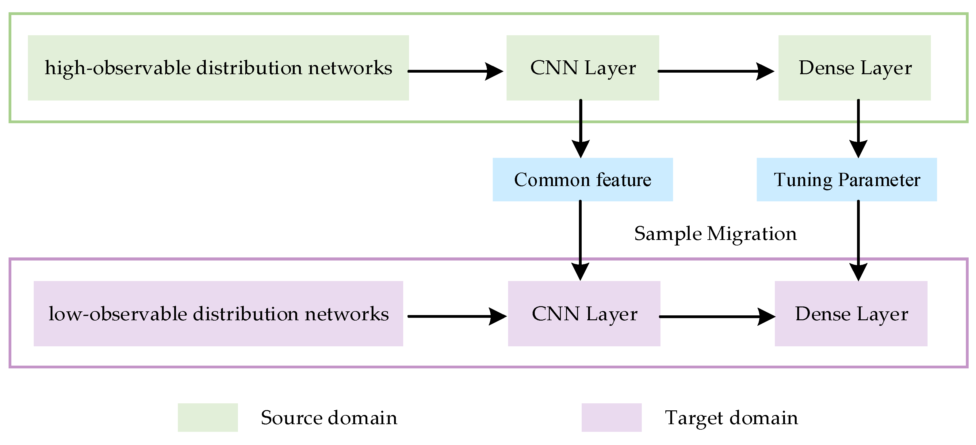
Under the assumption that two distribution networks have similar topologies, common features can still be extracted from their measurements, even if there is a significant difference in observability. This enables the migration of data from high-observable distribution networks to low-observable distribution networks. The specific sample migration process is illustrated in
Figure 1.
Among various neural networks, during model training, deep neural networks (DNNs) suffer from parameter explosion, while recurrent neural networks (RNNs) are prone to gradient vanishing and explosion. In contrast, convolutional neural networks (CNNs) leverage techniques such as shared convolutional kernels and local feature extraction, which offer powerful capabilities for feature extraction and nonlinear representation, effectively capturing essential information from input data. This paper constructs a CNN model to capture the nonlinear relationship between distribution network measurements and state variables. The model is capable of performing state estimation for distribution networks under varying operating conditions and network topologies. The convolutional layers (CNN layers) extract feature information from the input data by applying sliding convolutional kernels. The fully connected layers (Dense layers), placed after the CNN layers, transform the extracted feature information into the target output. During sample migration, CNN layers are frozen and the structure and network parameters of CNN layers are saved to extract common features, while parameters of Dense layers are tuned by using a small number of samples from the new topology. The backpropagation algorithm is used to learn the parameters of each convolution unit [
28]. Unlike other artificial neural networks (ANNs), CNN layers first process input blocks locally through convolution and then apply activation functions for further computation. The computational process of CNN can be described as:
where
and
are the input and output of a CNN layer, respectively.
denotes the state of distribution networks, and
,
,
signify measurement variables of distribution networks.
indicates the output of a convolution operation.
and
represent convolutional kernel and bias vector, respectively.
denotes the activation function, the introduction of which endows CNN with powerful nonlinear representation capabilities.
3.4. Algorithm Process of Proposed Method
This paper proposes a data-driven state estimation method based on sample transfer to tackle the issue of low-observable distribution networks being unable to perform state calculations normally. The specific process is demonstrated in
Figure 2.
During offline training, the state estimation model is trained using a historical database (source domain). The model’s input features include measurements of a distribution network described in
Section 3.1. In the online estimation stage, real-time measurements of the distribution networks are collected, and the integrity of these measurements is evaluated. If the measurement data are sufficient and the original model meets the estimation accuracy requirements, the input features are directly input into the trained model. Otherwise, the distribution networks serve as the target domain for feature extraction and transfer learning.
4. Case Study
Two actual 26-node distribution networks in a certain region are selected as test systems in this paper. According to the method proposed above, all 26-node distribution networks in the region are clustered into four typical topology sets. One topology type is selected, with the distribution networks featuring complete measurements serving as the source domain and the distribution networks with insufficient measurements as the target domain. Based on sample migration technology, the abundant samples in high-observable distribution networks are migrated to low-observable distribution networks.
Multi-time section power flow calculations are performed based on load curves which come from actual operational data of the region networks, and Gaussian white noise is added to node voltage amplitudes and node injection powers to simulate real-time measurements. The node voltage magnitudes generated by power flow calculations are used as the true values, while the WLS is applied for multi-time section state estimation to generate estimated node voltage magnitudes, which are used as labels for model training. This paper selects 4000 cross-sectional measurements for training the source domain model, with 3500 cross-sections used for model training and 500 cross-sections used for validating. For the low-observable distribution networks in the target domain, select the few section measurements of the low-observable distribution networks in the historical database, and based on the distribution networks sample migration technique, make the state estimation model of the source domain applicable to the distribution networks of the target domain.
This algorithm proposed above is implemented in Python, using the Keras module used to establish the state estimation model, specifically a convolutional neural network (CNN). After extensive testing, the CNN model is composed of three convolutional and two dense layers, with 32 samples processed per iteration and 60 training epochs. The simulations are conducted on a personal computer with an Intel(R) Core (TM) i5-8300H CPU @ 2.30 GHz and 8.0 GB of memory.
4.1. Test System Introduction
According to the distribution network topology modeling method introduced in
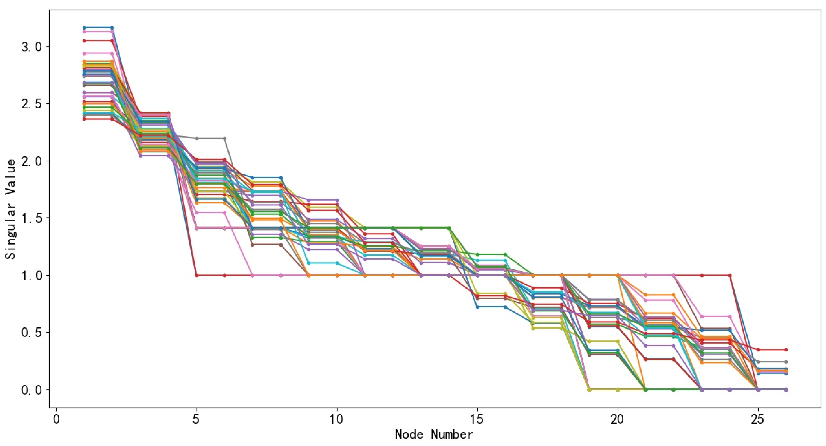
Section 3.2, all 26 node distribution network topologies in a certain region are clustered in this paper. Firstly, adjacency matrices are constructed for different distribution network topologies. Secondly, singular value sequences of each adjacency matrix can be calculated. Finally, based on the K-means clustering algorithm, these singular value sequences can be clustered to obtain typical topology sets for different distribution networks. The singular value sequence calculation results of the 26-node distribution network topology are shown in
Figure 3. Among them, lines of different colors represent singular value sequences of different distribution networks.
In order to determine the optimal number of clusters for the 26-node distribution network, the elbow method is used in this paper. As shown in
Figure 4, the vertical axis represents the error of clustering results and the horizontal axis represents the number of clusters. According to the elbow method, the optimal number of clusters for a 26-node distribution network is 4, each of which can be seen as the typical distribution network topology.
After completing the typical topology extraction of the 26-node distribution network, one type of the typical topology is selected to test the proposed method. Measurement redundancy is defined as m/n, where m and n represent the number of real-time measurements and state variables, respectively. In the same typical topology set, one distribution network with high measurement redundancy (measurement redundancy is 1.53) and one distribution network with low measurement redundancy (measurement redundancy is 0.87) are selected as the source and target domain, respectively.
Figure 5a illustrates the topology of a distribution network with high observability, referred to as the source domain, while
Figure 5b depicts the topology of a distribution network with low observability, referred to as the target domain. As can be seen from the diagram, the topologies of the two distribution networks are largely similar, but there are significant differences in the number of topological connections. Additionally, the target domain topology has a branch that is disconnected compared to the source domain. Therefore, during the sample migration stage, for the disconnected branch power flow measurements in the target domain, this paper supplements them with zeros to maintain consistency in feature dimensions during model training.
4.2. Estimation Accuracy Test
This paper uses the 26-node distribution network mentioned above to demonstrate the test results. Gaussian white noise is added to the true values as measurement data to evaluate the effectiveness of the algorithm under ideal conditions. The standard deviation of voltage amplitude is set to 0.005 p.u., and the standard deviation of electric power is set to 0.01 p.u. Additionally, to further demonstrate the performance of the algorithm, the amplitude and angle of the node voltage are displayed.
The maximum estimation error and the average estimation error are used as indicators to measure the effectiveness of the algorithm. The specific formulas are as follows:
where
and
represent maximum estimation error and average estimation error, respectively.
and
indicate the true value and the estimated value of
state variable at time
.
Figure 6 illustrates the comparison between the averages of the estimated and true values for all cross-sections at each node of the testing system. As seen from
Figure 6, the method proposed demonstrates excellent estimation performance in terms of both node voltage amplitude and node voltage angle, successfully achieving state estimation for the entire networks.
WLS is a widely used algorithm in distribution network state estimation, while WLAV effectively addresses the issue of bad data and offers strong robustness. Therefore, WLS and WLAV are chosen for comparison with the proposed algorithm.
Figure 7 and
Table 1 display the absolute error for node 5, evaluated using the proposed method, WLS, and WLAV. The figure presents the estimation results for 50 cross-sections.
The proposed SE algorithm has higher accuracy compared to WLS and WLAV in
Figure 5 and
Table 1. Compared to the WLS algorithm, the average absolute errors of node voltage magnitudes and node voltage phase angles are reduced by 58.07% and 55.60%, and the maximum absolute errors are reduced by 47.56% and 49.65%. Compared to the WLAV algorithm, the average absolute errors are reduced by 45.68% and 41.45%, and the maximum absolute errors are reduced by 32.70% and 36.93%.
The measurement redundancy in distribution networks affects the estimation results.
Table 2 presents the estimation results for low-observable distribution networks at different levels of measurement redundancy.
As shown in
Table 2, when the measurement redundancy decreases, the precision of the approach will be affected. The reason is that the method is model-based sample migration, which to some extent relies on the redundancy of instantaneous measurements. However, in the SE of low-observable distribution networks, the proposed method is significantly better than traditional algorithms.
4.3. Robustness to Bad Data
Affected by operating conditions and environmental factors, bad data inevitably exist in the measurement data input to distribution networks. In order to assess the robustness of the proposed approach, a 20% mixture of Gaussian error is introduced into historical measurement data to emulate the presence of faulty data in actual distribution networks. These augmented data serve as an additional training sample for the pre-training model. We assess the robustness of different algorithms by adding bad data (with an error standard deviation set to 3–10 times that of normal data) to the voltage amplitude measurements at nodes 2, 10, 15, and 22.
Figure 6 shows the average absolute error calculated by our algorithm, WLS, and WLAV for nodes with added bad data. In
Figure 8, the proposed method demonstrates good robustness in this case.
4.4. Calculation Efficiency
Traditional SE algorithms may encounter issues with complex models and low computational efficiency, and the computational efficiency decreases with the increase in system size. A data-driven method is used to enhance the efficiency of state estimation.
Table 3 presents the calculation times of different algorithms applied to various actual distribution networks.
As shown in
Table 3, when the testing system is small, the computation time of traditional SE algorithms (WLS, WLAV) and the proposed algorithm can all meet the real-time requirements of SE. In some cases, the computation efficiency of WLS and WLAV even outperforms that of the proposed method. However, as the system scale continues to expand, the computation time of WLS and WLAV significantly increases, while the computational efficiency of our algorithm remains largely unaffected by the system size. Therefore, the presented algorithm demonstrates better computational efficiency than conventional algorithms. The computation time for the proposed method refers to the online estimation time, while the model training is completed offline, without occupying online computing resources. Consequently, the online computation of the presented algorithm maintains good real-time performance.
5. Conclusions
This study addresses a data-driven state estimation based on sample migration for low-observable distribution networks. Based on sample migration technology, knowledge from high-observable distribution networks is transferred to low-observable distribution networks, enabling effective state estimation. Considering the results from the actual distribution network, the following conclusions can be drawn.
- (1)
In low-observable distribution networks, the proposed method enhances the estimation accuracy compared to traditional methods, such as WLS and WLAV. It effectively addresses issues of low estimation accuracy and estimation failure due to insufficient measurements in traditional methods. Additionally, it improves the model’s generalization ability.
- (2)
The method demonstrates better robustness and instantaneous performance in online SE compared to traditional WLS and WLAV. By incorporating bad data into the training samples and utilizing a data-driven SE model, the proposed approach shows superior performance in handling real-time estimation tasks.
Future work will consider system faults, variations in power sources and loads, and differences in line parameters, further extending the applicability of the proposed method.


