Characterization of Rock Pore Geometry and Mineralization Process via a Random Walk-Based Clogging Scheme

Abstract

Among the technologies for carbon neutral, CO₂ geological sequestration is one of the most promising. The mechanisms of CO₂ behavior within pore space are complex and influenced by multiple factors, with the geometric structure of porous formations being particularly critical to the technology’s efficiency. Among several important and challenging problems in geological sequestration, this work addresses the issue of selecting lithologies based on their geometrical structure. This study proposes a mathematical approach to characterize the geometric structure of porous rock and fluid flow using a random walk (RW) method. Our approach simulates the time evolution of particle flow through highly disordered and heterogeneous digital rock models under a pressure gradient imposed between inlet and outlet surfaces. Through RW simulations, a probabilistic model for mineralization via a clogging (pore-filling) model is introduced, to examine the accumulation of particles within porous structures over time: single-phase clogging and multiple-phase clogging. In single-phase clogging, the porosity decrease can be described as a monotonically non-increasing function of the deposition probability. However, this is no longer true in the multiple-phase strategy because large deposition probability blocks the capillaries near the inlet surface, preventing the fluid from easily invading easily the outlet. In this study, numerical studies conducted on four types of natural rocks—Bentheimer, Doddington, Estaillades, and Ketton—revealed that Ketton exhibits the highest permeability. Our results suggest that Bentheimer, Doddington, and Ketton formations are suitable candidates for CO₂ sequestration, while Estaillades is less favorable from a geometric standpoint. The methods presented in this work contribute to effectively identifying natural rocks with geometric structures advantageous for CO₂ storage.

1. Introduction

Carbon capture, utilization, and storage (CCUS) is a process where a relatively pure stream of carbon dioxide from large point sources, such as fossil fuel power plants or industrial facilities (cement, iron, steel, etc.) is separated, treated, and transported to a long-term storage location. Geological carbon dioxide sequestration is considered a promising technology in CCUS for reducing carbon emissions into the atmosphere by injecting it into natural geological formations, such as saline aquifers, oil and gas reservoirs, and deep coal beds, and storing it permanently and safely there. To achieve carbon neutral, furthermore, we should also consider the negative emission scheme that captures CO₂ directly from the atmosphere and stores it in a geological formation. The security and the efficiency of CO₂ storage are ensured by several trapping mechanisms [1], including structural and stratigraphic trapping geological storage [2], capillary trapping [3], solubility (dissolution) trapping [4], and mineral precipitation (chemical reaction) [5,6].

The mechanisms of geological sequestration depend on the interplay between the geomechanical, thermal, hydraulic, and geochemical processes occurring as injected CO₂ migrates dissolve in formation fluid and react with formation bedrock. This is strongly influenced by several different factors, such as the injection fluid flow (e.g., injection rates, fluid topological characteristics), fluid properties (e.g., wetting or non-wetting, fluid–fluid interfacial tension [7]), the characteristics of porous material (e.g., pore morphology [8]), and wettability [9]. Even though advanced imaging technologies have been able to provide detailed information on fluid distributions in pore spaces in experiments [10,11,12], this process is time-consuming, costly, and effort-expensive. This is where mathematical modeling shines. Effective mathematical models can simulate a broad range of reservoir-relevant conditions within an acceptable period with the aid of the rapid improvement in computational resources [6,13,14,15].

In digital rock modeling, a clogging model is a computational approach used to study how fluid flow through porous rock formations becomes obstructed over time, due to the accumulation of particles, minerals, sediments, or other materials. This process is particularly relevant to applications such as geological sequestration, petroleum engineering, hydrogeology, and filtration systems. Clogging occurs when particles suspended in the fluid accumulate within the pore spaces, reducing permeability and impeding fluid flow. The clogging process involves two key components: particle transport and deposition mechanisms. Particle transport refers to the movement of particles within the fluid as they navigate through the pore spaces, while deposition mechanisms model how particles become trapped, stick to pore walls, or aggregate within pores. Common deposition mechanisms include mechanical trapping, surface adhesion, and bridging (where large particles span pores). By simulating clogging behavior, the model helps predict how porous formations evolve over time under fluid flow, allowing for improved reservoir management and a deeper understanding of long-term permeability changes in natural porous media.

Investigating the influence of the geometric structure of porous space is crucial for understanding fluid flow and clogging dynamics in digital rock models. The shape, size, and connectivity of the pores directly dictate how fluids move through the material, affecting both permeability and the likelihood of clogging. Complex pore geometries, characterized by varying pore throat sizes and irregular structures, create heterogeneous flow patterns, leading to regions of high or low flow velocity. These variations can significantly influence particle deposition and aggregation, which are primary drivers of clogging. By analyzing how the intricate geometry of the porous space impacts flow resistance and clog formation, it becomes possible to more accurately predict permeability reduction and develop optimized strategies to mitigate clogging in geological sequestration. This geometric insight is essential for lithology selection in CO₂ storage technology, ensuring the long-term efficiency and stability of storage reservoirs.

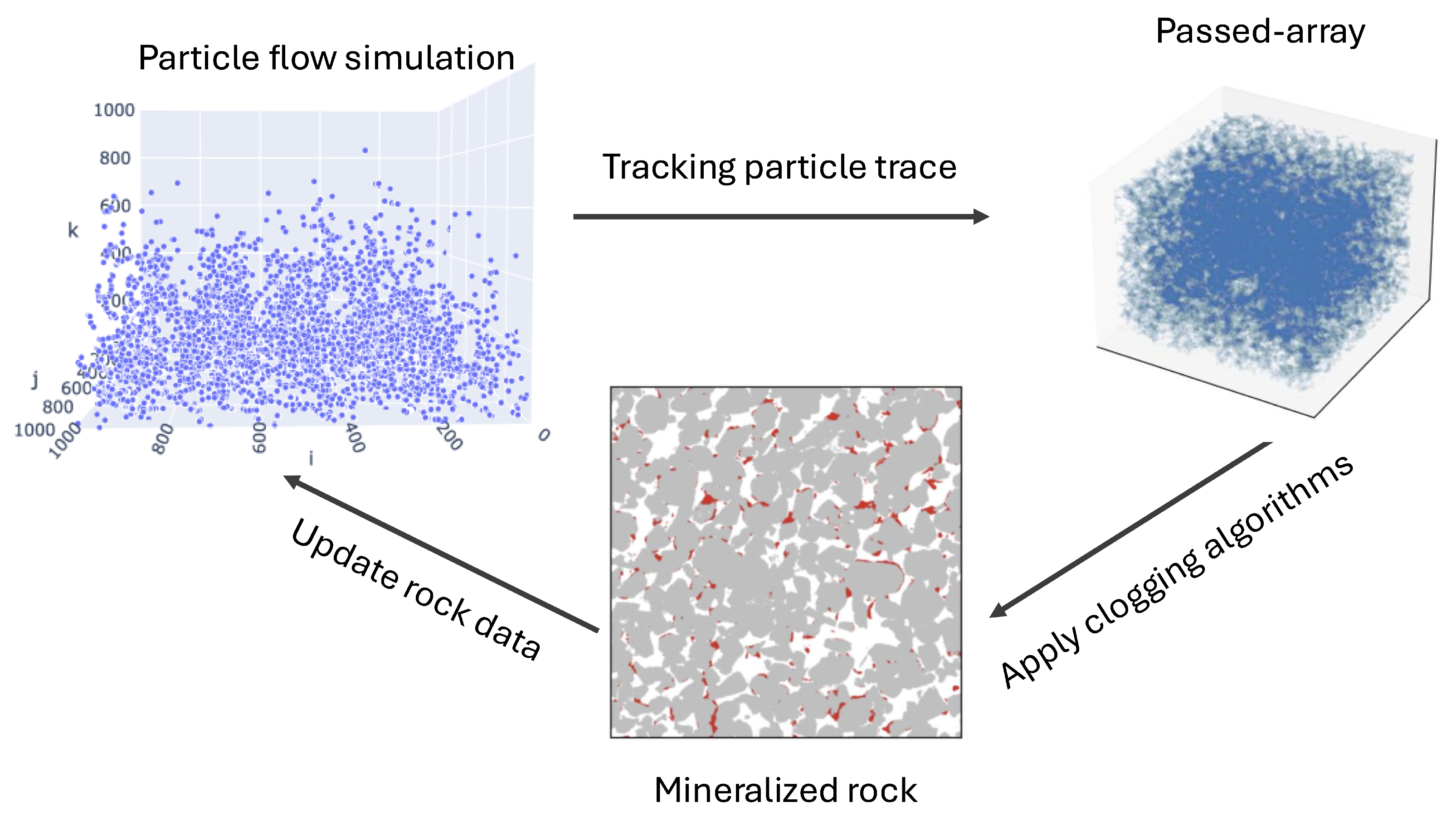
In this paper, we aimed to investigate the effect of the geometric structure of natural rock formations on fluid flow through pore spaces and the clogging process. We began by analyzing the geometrical characteristics of pore spaces in four types of natural rock models, examining factors such as porosity, pore size distribution, and the degree of pore voxel interconnection. We then proposed a random walk-based method to simulate the fluid flow dynamics of particles in complex pore structures, driven by pressure applied between the inlet and outlet surfaces. We proposed a probabilistic clogging model based on the particle transport algorithm, introducing two strategies: single-phase and multi-phase clogging. In single-phase clogging, porosity decreases monotonically as a function of deposition probability, whereas in multi-phase clogging, structural changes disrupt this monotonicity. High deposition probabilities lead to rapid clogging, narrowing capillaries and hindering particle transport. This method offers a valuable tool for selecting rock formations for geological sequestration. A schematic diagram representing the workflow is depicted in Figure 1:

Theoretically, the fluid dynamics in porous materials can be modeled by different mathematical formulas, depending on the characteristics of the fluid and the porous media. For example, Darcy’s law governs the slow flow in a fully saturated porous medium, and Richard’s equation governs the flow in a variably saturated porous medium. Traditional computational fluid dynamics (CFD) methods [16,17], which numerically solve macroscopic properties conservation equations, are highly accurate for macroscopic systems and complex dynamics but require significant computational resources and are less intuitive for stochastic or microscopic systems. In the lattice Boltzmann method (LBM) [13,18], instead of solving Navier–Stokes equations directly, fluid density on a lattice is simulated with flow and collision (relaxation) processes. The LBM has been used widely to simulate single- and multi-phase flow behavior within the true pore geometry of porous media [19,20,21,22]. The LBM is a versatile mesoscopic approach that balances accuracy and computational cost but can struggle with extreme heterogeneity.

Unlike these CFD approaches, the random walk method models transport processes as the movement of individual particles or agents. This discrete and probabilistic approach offers new possibilities for simulating complex systems with inherent stochasticity. Diffusion is naturally represented through Brownian motion within the random walk framework, providing a direct and intuitive alternative to the discretization of partial differential equations (PDEs). Moreover, the method eliminates the need for computational grids, avoiding challenges such as mesh generation and grid resolution, particularly in heterogeneous structures like porous rocks. In other words, the random walk method operates directly on the digital rock models without requiring manual approximations. Notably, the concept of using random walk to simulate the clogging process within pore formations was first introduced in [23]. However, this approach was previously implemented in a free, two-dimensional environment. To our knowledge, no comprehensive study of real three-dimensional natural porous rocks has been explored yet.

Like LBM, our random walk approach also effectively simulates the fluid flow within a real pore medium, thanks to its three advantages: all calculations are local, there is no need for complicated procedures for interface tracking, and the scheme is explicit. The main difference between our approach and the approach using LBM in [13] is that in the mentioned work the LBM is used to simulate the displacement of a wetting liquid fluid, e.g., H₂O, by a non-wetting liquid fluid, e.g., CO₂. In our random walk approach, we cannot consider pressure information on fluid flow calculation directly. Therefore, we cannot evaluate fluid displacement characteristics that are available in the LBM approach [24]. On the other hand, the random walk approach allowed us to easily model the clogging process (i.e., mineralization modeling) and use larger digital rock models, due to fewer computations compared to LBM. We simulated the particle fluid flow in the porous space of different types of rock formations, to choose the most geometrically favorable porous formation among the candidates for geological storage. We performed the simulations on three-dimensional natural porous rock samples (of $1000\times 1000\times 1000$ voxels), which were 15 times larger than those in [13] ($320\times 320\times 640$), in the sense of the number of grid points.

Based on the particle transport results, we developed a stochastic clogging model to capture the probabilistic nature of the particle deposition and accumulation. The likelihood of a void voxel becoming clogged during fluid transport depends on the number of times that the void voxel has been visited by particles and on a predefined parameter known as the deposition probability. As the clogging process advances, fewer pathways remain open for fluid flow, leading to a gradual change in the geometric structure of the pore space. This, in turn, results in a progressive reduction in both the formation’s overall permeability and the efficiency of the fluid injection. The impact of deposition probability on clogging processes is quantified by modeling the decrease in porosity as a function of deposition probability, using the curve-fitting method. The coefficient of the fitted curves for different rock types highlights the potential of certain rocks for carbon storage, particularly from a geometric standpoint.

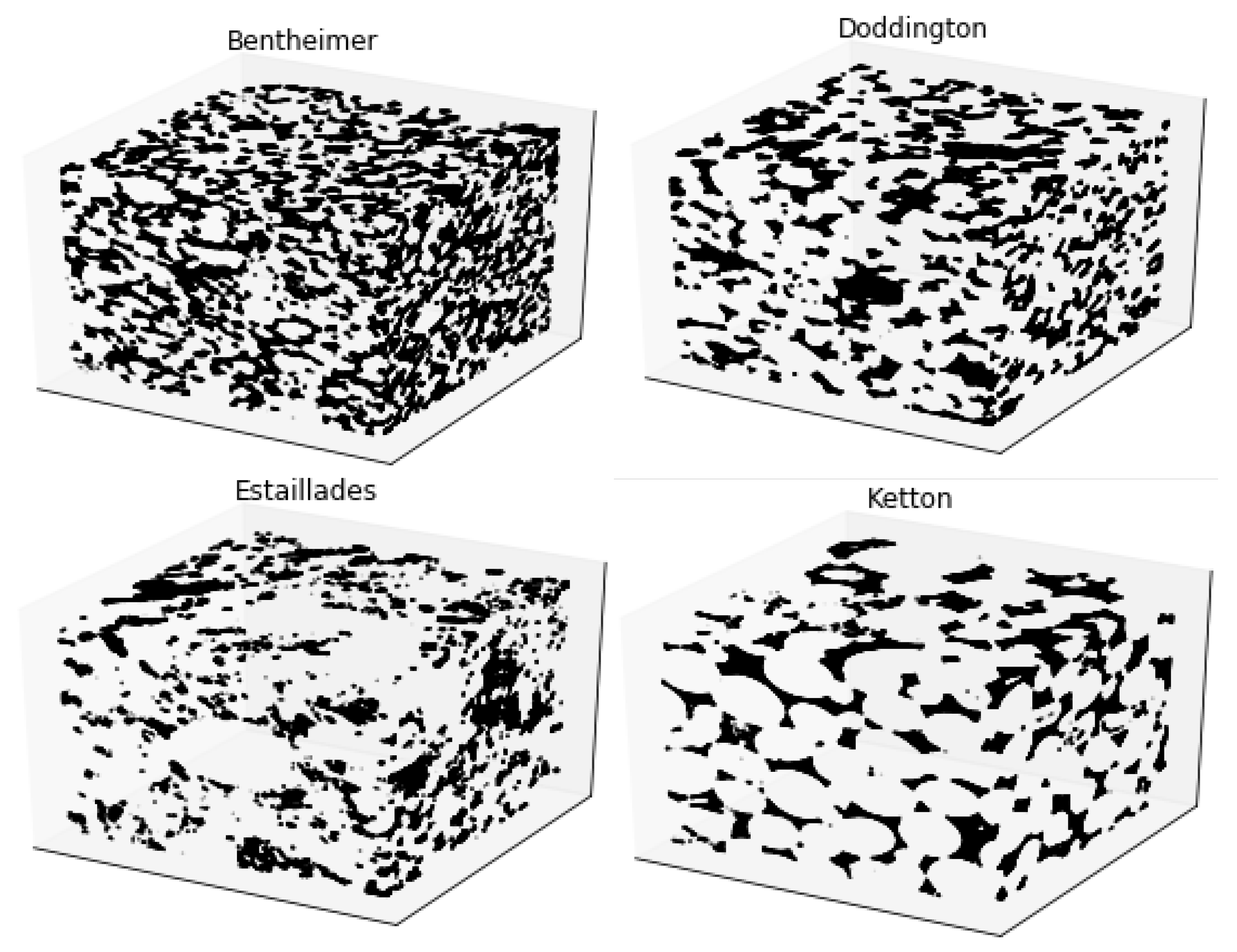
The outline of the paper is as follows. Section 2 describes the four digital rock models used in this study and introduces a graph-based representation approach to analyze the important geometrical properties of pore spaces—including porosity, degree of pore voxels, and connectivity—that are critical for transport in porous media. In Section 3, we present the random walk rule for simulating particle movement within the pore spaces of rock formations under the pressure gradient imposed between the inlet and outlet surfaces. Section 4 introduces our proposed stochastic clogging (pore-filling) model, which simulates particle accumulation in pore spaces over time. Section 5 presents the numerical results and interpretation for the particle transport (Section 5.1) and clogging models (Section 5.2). The paper concludes with our conclusions and future perspective in Section 6.

The simulations in this work were implemented in Python with the aid of several third-party libraries, such as Numpy [25], Scipy [26], Matplotlib [27], and Porespy [28].

2. Digital Porous Rock Models and Graph-Based Representation

2.1. Materials

The process of obtaining the sample data is described as follows. After a rock sample was collected, a microcomputer tomography (CT) scanner was used to take pictures of multiple slices of the rock. The CT image then went through a Gaussian smoothing process, in order to reduce high-frequency noise and adjust the contrast, resulting in a gray-scale image. The third step was the segmentation process: a single gray-scale threshold was chosen, so that the porosity of the sample matched the experimental porosity of the rock type under investigation, transforming the gray-scale image into a binary image, illustrated in Figure 2:

2.2. Graph-Based Representation of Pore Space of Digital Porous Rock Models

We analyzed the geometric structural properties of the pore spaces within the sample rock data, such as the porosity, distribution of pore sizes, degree of pore voxels interconnection critical to the particle flow, and the clogging process. Some statistical measurements of the geometric structural properties of the pore spaces are given in

Table A1. Statistics on pore structure.

	Bentheimer	Doddington	Estaillades	Ketton
Porosity	21.7%	19.6%	12.7%	13.3%
Number of connected components	33,920	280	14,832	39,190
Number of connected components having points on inlet surface	159	10	98	123
Number of pore voxels on inlet surface	210,365	216,086	100,175	135,832
Number of passable components	1	1	1	1
The proportion of passable component’ voxels on inlet surface over total pore voxels on inlet surface	98.262%	98.460%	69.169%	97.498%
Proportion of passable component over total pore space	99.764%	99.484%	85.668%	99.002%

in Appendix A.

The degree of pore voxels interconnection can be quantified by pore-connected components. A connected component is defined as a maximal subset of pore voxels, such that there is a path through the pore spaces connecting any two voxels within that component.

To explain this precisely, we need some mathematical notations, as follows. We embed the rock sample into the three-dimensional Euclidean space, having three standard basis vectors, $\overrightarrow{i}=(1,0,0),\overrightarrow{j}=(0,1,0),\overrightarrow{k}=(0,0,1)$. Given a pore voxel x at the lattice position $(i,j,k)$ at time instant t, we define its lattice 6-neighbors as

$$\mathcal{N}\left(x_t\right)=\{(i\pm 1,j,k),(i,j\pm 1,k),(i,j,k\pm 1)\}.$$

(1)

Let $\mathcal{V}$ be the set of all the pore voxels; we define the pore neighbors of a pore voxel as

$${\mathcal{N}}_p\left(x_t\right)=N\left(x_t\right)\cap \mathcal{V},$$

(2)

where ∩ is the intersect operator on sets. Each pore voxel’s number of pore neighbors is called its degree. By the above pore neighbors construction, pore voxels will take degree values in the set $\{0,1,2,3,4,5,6\}$. A pore voxel having degree 6 lies in the inner part of the pore space, while those with other values of degree lie on the boundary of the pore space. The pore voxels with degree 0 are isolated: that is, a particle from this position cannot go anywhere else, and a particle from anywhere else cannot arrive at this position. There are quite a large number of isolated pore voxels in Bentheimer and Ketton. The pore degree counts of the four rock samples are given in

Table A2. Pore degree distribution of rock samples.

Degree	Bentheimer	Doddington	Estaillades	Ketton
0	18,423	0	1206	20,238
1	240,306	2226	15,185	84,971
2	1,507,674	97,880	334,002	325,845
3	8,634,944	5,727,949	6,377,542	3,846,226
4	11,366,579	7,120,937	7,501,411	4,657,615
5	17,306,204	11,974,797	11,766,153	7,362,755
6	177,699,440	170,884,266	101,316,974	116,745,140

.

For each rock sample, we can construct a graph $G(\mathcal{V},\mathcal{E})$ on the vertex set $\mathcal{V}$ of pore voxels and the edge set $\mathcal{E}$, each of which connects two pore voxels in $\mathcal{V}$. We say that there exists an edge $(x,y)$ that connects two pore voxels x and y if x and y are in the pore neighbor of each other. Note that if the pore voxel x is in the pore neighbor of the pore voxel y, then y is also in the pore neighbor of the pore voxel x; therefore, the graph is undirected. We say that there is a path connecting the two voxels $x_1$ and $x_n$ if there exists a sequence $(x_1,x_2,x_3,\dots ,x_n)\in {\mathcal{V}}^n$, such that $(x_i,x_{i+1})\in \mathcal{E}$ for $i=1,2,\dots ,n-1$. Two pore voxels x and y are said to be connected if there exists a finite path connecting them. From this construction, the pore-connected components are the connected components of the graph $G(\mathcal{V},\mathcal{E})$. By definition, the connected components are disjoint and their union is the set $\mathcal{V}$. In our simulation, we developed a tree-based searching–tracking algorithm to classify the pore spaces into disjoint connected components.

The number of pore-connected components varies for the four rock types. We observed that only in Doddington were there quite a few pore-connected components while in the other three samples the pore spaces were comprised of a large number of connected components; see Table A1 in Appendix A.

In this study, we wanted to investigate the efficiency of particle transport and clogging processes for different types of natural porous rock formations; it was, therefore, important to know if the particle flow injected from the inlet surface could invade deep into the rock, at least to the outlet surface. Therefore, we introduced the notion below.

A passable component is a pore-connected component containing points on the inlet surface and points on the outlet surface.

By the above definition, the particles could only travel from the inlet surface to the outlet surface through the passable components. Among many connected components, it was interesting that each rock had only one passable component, which accounted for the majority of the pore spaces in the rock data (see Table A1).

3. Particle Flow Through Pore Space Governed by Random Walk

This section proposes a method to investigate the particle flow through the pore space of the rocks under the pressure gradient imposed between the inlet surface and the outlet surface. To make the embedded coordinate specific, we put the samples into a three-dimensional Euclidean space, so that the inlet surface is on the space $k=0$, with four corners, at $(0,0,0)$, $(1000,0,0)$, $(0,1000,0)$, and $(1000,1000,0)$, and the outlet surface is on the space $k=1000$, with four corners, at $(0,0,1000)$, $(1000,0,1000)$, $(0,1000,1000)$, and $(1000,1000,1000)$.

3.1. Particle Injection

As initializing, a number, K, of particles are injected into the inlet surface of the rock sample under the imposed pressure gradient toward the direction from the inlet to the outlet surfaces, which we also called the injection direction. These particles will invade deeply into the pore space through the pore voxels on the inlet surface. In the simulation, the K pore voxels in the inlet surface were randomly chosen following the uniform distribution, with replacement, i.e., one pore voxel could be chosen several times to be the initial position of particles. Note that in our simulations we allowed multiple particles located at a single pore site, because the grid size was approximately ${10}^4$ times larger than the diameter of the particles.

The movement of the particles follows the random walk algorithm described in the following subsection. The inlet surface only allows the particle to go in, not to go out, and the injected particles can only escape through the outlet surface, as the other surfaces are made impermeable. In order to simulate the impermeability on these surfaces, we add an artificial grain layer adjacent to each of these surfaces outside of the rock sample. Because of this, the size of the rock in the simulation was ${(1000+2)}^3$ instead of ${1000}^3$. With this technical trick, the lattice 6-neighbors are well-defined for each particle in the pore voxels, because the particle cannot go to the outermost layers where all the voxels are grains.

3.2. Random Walk Rule Governing Particle Movement

The random walk method is especially appropriate for describing particle movement in highly disordered and heterogeneous, large-scale media, such as the natural porous formation being studied in this work. The classical random walk particle schemes rely on the equivalence between the Langevin equation and the advection–dispersion equation [30,31]. This method usually requires high computational costs when there exists low permeability or low-velocity areas in the media when the particles remain trapped in low diffusion zones. The efficiency of the particle-tracking algorithm can be enhanced drastically by moving a particle over a fixed distance imposed by the computational mesh [32,33]. Variants of this methodology are continuous time random walk (CTRW) and time domain random walk (TDRW). It has been shown that the discretized advection–dispersion equation and the TDRW are equivalent [34,35]. The TDRW in general moves particles on a lattice with jumps of fixed distance, with the direction and transition time being determined by the local advection and dispersion.

In this work, we formulated a TDRW model to describe the particle flow within the porous media under the pressure imposed between the inlet and the outlet surface in the presence of the clogging process. Therefore, the model introduced here works in time-dependent random environments, because the geometric structure of the pore space evolves during the deposition process in a stochastic way. The proposed method, though simple, is very powerful, and it has the potential to be applied to a variety of complex large-scale disordered phenomena arising from physics, biology, and engineering; for example, the propagation of heat or diffusion of matter through a medium that is highly irregular, due to defects, impurities, or fluctuation.

At a given time instant t, suppose that a particle x is at the position $(i,j,k)$, with the increasing of the third coordinate $\left(k\right)$ representing the injection direction from the inlet to the outlet. In this case, we can identify $x_t\equiv (i,j,k)$. The particle can either stay still or move to one of its pore neighbors defined in Equations (1) and (2).

Only when ${\mathcal{N}}_p\left(x_t\right)=\varnothing$, with ∅ representing the empty set, i.e., $x_t$ has degree 0, will the particle x stay still. Otherwise, it will randomly move to one of its pore neighbors in ${\mathcal{N}}_p\left(x_t\right)$ in the next time instant $t+1$, with the following transition probability:

$$p(x_t\to y)={\displaystyle \frac{g(x_t,y)}{{\displaystyle \sum _{z\in {\mathcal{N}}_p\left(x_t\right)}}g(x_t,z)}},$$

(3)

where

$$g(x_t,z)=\left\{\begin{array}{cc}v+d\hfill & \mathrm{if}{x}_t\to z\mathrm{is}\mathrm{injection}\mathrm{direction}\hfill \\ d\hfill & \mathrm{otherwise}.\hfill \end{array}\right.$$

(4)

Here, v is called velocity, which models the pressure gradient, and d is the dispersion. Both v and d are chosen to be non-negative. The positive velocity v ensures that the particles have more tendency to move in the injection direction than in any other direction. In this sense, the parameter v can indirectly characterize for the strength of the pressure. The probabilistic jumping rule specified in (3) and (4) models both the advective and diffusive terms. Moreover, the transition probability is spatial-dependent, due to the heterogeneity of the pore structure. From the above construction, the transition probability $p(x_t\to y)$ of the particle is specified as in

Table 1. Transition probability of particles $p(x_t\to y)$ at each random walk iteration t. Here, ${\mathcal{N}}_p\left(x_t\right)$ denotes the pore neighbor set of the voxel in which a particle is located at time t, and ∅ denotes the empty set.

	${\mathcal{N}}_{\mathit{p}}\left({\mathit{x}}_{\mathit{t}}\right)=\mathit{\varnothing }$	${\mathcal{N}}_{\mathit{p}}\left({\mathit{x}}_{\mathit{t}}\right)\ne \mathit{\varnothing }$
$y=x_t$	1	0
$y\in {\mathcal{N}}_p\left(x_t\right)$	0	specified as in (3) & (4)

:

There are several key assumptions commonly made in the random walk method: independent particle motion, uniform medium properties, discretization of time and space, neglect of convection or external forces, simplified boundary conditions, and neglect of particle size and shape. Each assumption has its advantages and disadvantages; see

Table 2. Key assumptions in RW method, along with their advantages and disadvantages.

$\mathbf{Assumption}$	$\mathbf{Advantage}$	$\mathbf{Disadvantage}$
Independent particle motion	Simple to implement, suitable for particle-level simulations.	Ignores particle–particle interactions, limiting applicability to systems where interactions matter.
Homogeneity of medium	Flexible for uniform media.	Poor representation of spatial heterogeneity without additional modifications.
Discretization	Simplified computation with adjustable step size.	Accuracy depends on step size; may introduce artifacts when the physical scale is not well aligned.
Neglect of convection/forces	Ideal for diffusion-dominated systems.	Limited applicability to systems with significant advection or external forces.
Simplified boundary conditions	Handles simple boundary conditions well.	Struggles with complex or dynamic boundaries without extensive customization.
Neglect of particle size/shape	Simplified by treating particles as point-like.	Does not account for finite size or shape effects, affecting accuracy in systems with size-sensitive phenomena.

. For example, recall that the classical random walk relies on the Langevin equation, which describes the movement of the non-interacting particle due to advection and uncorrelated random velocity. Thanks to this independence, we can parallelize our algorithms; that is, we can run a large number of particle movements simultaneously, which offers a remarkable advantage in terms of computational time.

The above limitations are acceptable for the purpose of characterizing the geometric structure of porous formation. For future research, several approaches could help address these limitations and improve the accuracy of CO₂ penetration prediction. These include introducing rules for particle–particle, particle–medium interactions such as collision dynamics and hydrodynamic forces, hybrid approaches that combine the random walk method with continuum models to address multiscale and anisotropic effects, and comparing the predictions of the random walk model with experimental data or more detailed simulation, to identify when its assumptions hold.

4. Clogging Models

Clogging refers to the process in which particles suspended in the fluid (e.g., fine particles, minerals, or sediments) accumulate in the pore spaces, reducing permeability and impeding fluid flow. This process can be driven by size, shape of particle, concentration, and the velocity of the fluid. In this section, we propose a new clogging (pore-filling) model to elucidate the effect of geometry structure on the fluid flow through the pore space of media.

In the literature, there are a few works that propose clogging models, e.g., [6,36,37,38]. Keehm et al. determined the four classes of pore-filling mechanisms: grain–pore boundary, low-flux, high-flux, and random filling. This pore-filling mechanism is controlled by fluid rates. In [6], the authors introduced the CT image threshold adjustment model and the reactive transport clogging model to estimate the pore structure changing due to carbonate precipitation. The latter model uses chemical reaction theory to evaluate the local volume variation of the precipitate, with the assumption of CO₂ equilibrium conditions; that is, the authors considered the divalent cations’ concentration that is derived by solving the reactive transport model.

In this work, to elucidate the role of geometric structure, we address the dynamics of particle deposition—the spontaneous attachment of particles to surfaces by means of the probabilistic clogging model.

At the initialization step, a total of K particles are injected into the inlet surface of the rock samples. They invade through the pore spaces in the rock formation, under the pressure imposed between the inlet and the outlet surface, following the random walk rule introduced in Section 3.2. During the particle flow process, we construct the passed array, as described below.

The passed array is a one-dimensional array of length equal to the total number of pore and grain voxels in the rock sample, which keeps track of the number of times the particles have passed through each voxel during the random walk process.

Because the length of the passed array is the same as the flattened rock sample, it also keeps track of the corresponding voxels’ positions in the rock sample. As the particles cannot move to the grain voxels’ positions, the elements corresponding to grain voxels on the passed array are always 0 s. By utilizing this, we reduce the memory usage by storing the passed array in a sparse matrix.

At some given time instants, the pore voxels will become grain voxels, with the probability given by

$$f(q,n)=\sum _{i=1}^n{(1-q)}^{i-1}q\equiv 1-{(1-q)}^n$$

(5)

where $q\in [0,1]$ is the probability of deposition, and where n is the number of times that particles have passed through the corresponding void position. The value of n is specified by the corresponding element in the passed array. It is easy to verify that the expression in (5) satisfies the requirements of a probability measure as $f(q,n)\in [0,1]$ for any $q\in [0,1]$ and that $n=1,2,3,...$ and $f(q,n)$ tends to 1 as n approaches infinity.

To understand the mathematical meaning of the expression (5), let us consider a sequence of i Bernoulli experiments $(X_1,X_2,\dots ,X_i)$, which is also called a Bernoulli process. The Bernoulli trials $X_j,j=1,2,\dots ,i$ take either the value 1 if the experiment succeeds with probability q or 0 if the experiment fails with probability $1-q$. Then, the probability of the output $(0,0,0,\dots ,0,1)$, i.e., that the experiment fails on all first $i-1$ trials and succeeds at the last trial i, is ${(1-q)}^{i-1}q$. Similarly, each element in the finite series (5) represents the probability of a pore voxel being precipitated at the time instant when the number of times a particle visits that position is exactly i and failing to be precipitated at all $i-1$ previously visited times. Therefore, the probability of a pore voxel that has been visited n times being precipitated is the sum of all the probabilities that it is precipitated at any time $i=1,2,\dots ,n$ during the random walk process. This is equivalent to 1 minus the probability that the pore voxel fails to be precipitated n times (the right-hand side in (5)). In the following, we propose two clogging algorithms: single-phase and multi-phase.

4.1. Single-Phase Clogging

On the single-phase strategy, after the fluid flow simulations finish, either when the prescribed number of the maximum simulation steps is reached or when all the particles have escaped from the outlet surfaces, we apply the deposition rule (5) once to update the states of the voxels on the rock, where some of the pore voxels change to grain voxels, making the porosity decrease. This procedure is described in Algorithm 1:

Algorithm 1 Single-phase clogging

1: procedure Single-phase clogging($K,v,d,N,q$) Input: pore rock sample Parameter setting: 2:     K: number of injected particles, 3:     v: velocity, 4:     d: dispersion, 5:     N: maximum number of random walk, 6:     q: probability of deposition. Initialize positions of K particles by uniformly random choosing from pore voxels on the inlet surface. Initialize the passed array whose elements are all 0s. $n=0$ 7:     while $n<N$ and there exist particles in the pore space do 8:         $n=n+1$ 9:         Update particle positions according to (3) and (4). 10:         Update passed array. 11:         Remove particles that have reached the outlet surface. 12:     end while Perform deposition based on passed array according to (5). Update rock sample. return Updated rock data. 13: end procedure

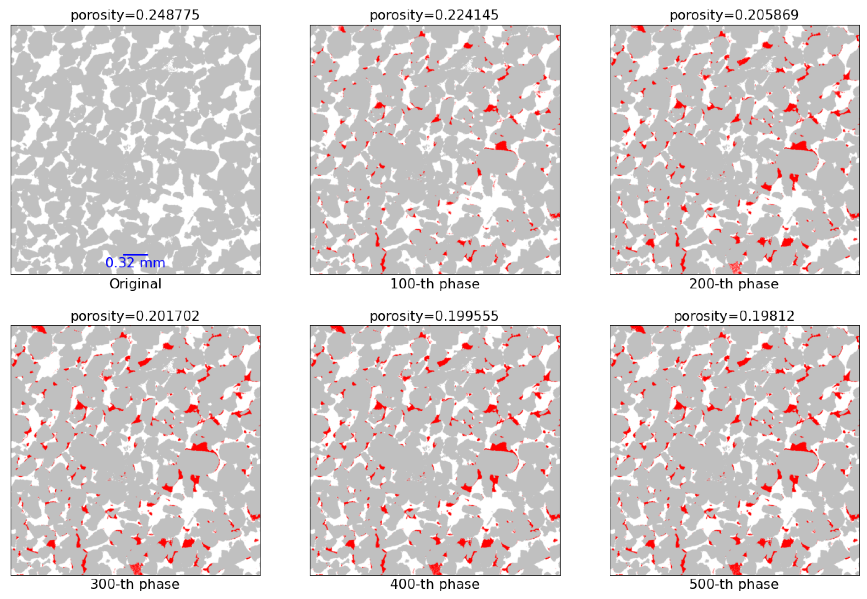
4.2. Multi-Phase Clogging

Multi-phase clogging is a consecutive sequence of single-phase clogging. In parameter setting, we predetermine the number of phases to perform. At the end of each phase, some pore voxels become grain voxels because of the deposition; therefore, the porosity and the geometric structure vary. During the simulation process, we use a one-dimensional array, called the position array, to keep track of the position of the particles injected into the pore spaces, and we remove the element from the array when some particles escape from the outlet surface. In addition, at the end of each phase i, the particles that are presented at the precipitated pore voxels will also be removed from the array.

The updated rock data after the deposition process at the end of phase i will be used as the domain for the simulation in phase $i+1$. We count the number of particles that are still present in the pore space of this new rock (the length of the array containing the positions of particles in the last step); then, we inject new particles to the inlet surface of the new rock, if necessary, to ensure that the number of particles in the position array at the beginning of each phase is exactly K (predefined parameter). This is a variant of the periodic boundary condition, which ensures the preservation of the number of particles at the beginning of each phase. The passed array is also updated at the end of each phase.

The iteration process finishes when the predefined number of phases is reached. The multi-phase clogging procedure is summarized in Algorithm 2:

Algorithm 2 Multi-phase clogging

1: procedure Multi-phase clogging($K,v,d,N,q,M$) Input: pore rock sample Parameter setting: 2:       K: number of injected particles, 3:       v: velocity, 4:       d: dispersion, 5:       N: maximum number of random walks, 6:       q: probability of deposition, 7:       M: number of phases. Initialize positions of K particles by uniformly random choosing from pore voxels on the inlet surface. Initialize the passed array whose elements are all 0s, and initialize the position array as empty. 8:         for m = 1:M do 9:            if Number of particles within the pore space is less than K and there exist pore voxels on the inlet surface then 10:              Inject more particles to the inlet space, such that the number of particles within the pore space is exactly K. 11:               Update position array. 12:         end if 13:         $n=0$ 14:         while $n<N$ and there are particles within the pore spaces do 15:            $n=n+1$ 16:            Update position array according to (3) and (4). 17:            Remove particles that have reached the outer surface. 18:            Update passed array. 19:         end while 20:         Perform deposition based on passed array according to (5). 21:         Remove particles at the position of precipitated points. 22:        Assign values 0s to the elements in passed array corresponding to the precipitated pore voxels. 23:         Update pore rock. 24:     end for return Updated rock data. 25: end procedure

5. Results and Interpretation

5.1. Fluid Flow Invading

A total of $K=100,000$ particles is injected into the inlet surface of each rock sample, following the scheme described in Section 3.1. Under the pressure gradient imposed between the inlet and the outlet, these particles will move deeper into the pore spaces. The velocity and dispersion parameters were chosen as $v=1$, $d=0.01$ in this study. The simulations are performed for a total of 5000 time steps. With this setting, as $v>>d$, the particles have a much stronger tendency to move along the injection direction compared to the others. In the free lattice—that is, without the grain voxels—the expected position of a particle after 5000 simulation steps along the injection direction is

$$\left[(-1)\times {\displaystyle \frac{d}{v+6d}}+1\times {\displaystyle \frac{v+d}{v+6d}}\right]\times 5000={\displaystyle \frac{5000v}{v+6d}}\approx 4717.$$

When considering the movement along the injection direction, only the position transfer forward and backward along the k-coordinate needs to be counted, because movement along the $i,j$-directions does not contribute. However, as the porous rock samples we used in this study contained a large number of grain voxels, i.e., a small proportion of pore voxels (see Table A1) the speed of fluid flow along the injection direction was much lower. This is illustrated in

Table 3. Average propagation depth after the 5000th step of the RW simulation. It was calculated by taking the average of the z-coordinate of the particles at the 5000th time step. The corresponding coordinates of the escaped particles were assigned a value of 1000.

	Bentheimer	Doddington	Estaillades	Ketton
Average propagation depth	108	114	72	212

, which represents the measurements of the average propagation depths of the particles at the 5000th step of the random walk (RW) simulation. As shown in the table, the average propagation depth in Ketton is twice that of Bentheimer and Doddington, and three times of that of Estaillades.

Figure 3 shows samples of the evolution of fluid invading the pore spaces of the rock. During the random walk movement, the particles that reached the outlet surfaces were removed from the simulation for the next random walk step, as they were considered to have escaped. At the end of the simulations, there were no particles escaping from the outlet surface of Bentheimer and Estaillades, while in Doddington and Ketton the numbers of escaped particles were 5 and 581, respectively. Comparing the invading evolutions, we see that among the four rocks, the propagation of the particles along the injection direction increased from Estaillades to Bentheimer to Doddington and, finally, to Ketton. We further investigated the distribution of particles along the injection direction at the end of the simulations, i.e., $t=5000$. Figure 4 shows the kernel density estimates for the distributions. The log scale was used to better distinguish the differences, especially in the long tails of the distributions.

To quantify this propagation, we counted the number of particles present at several slices along the injection direction ($k=50;100;150;\dots ;1000$) according to the simulation time ($t=200;400;600;\dots ;5000$). As the random walk was stochastic, we used the aggregate (average) results on multiple (10) trials to access the robustness of the propagation on each rock sample. Figure 5 illustrates the flow propagation of the particles along the injection direction in the the pore spaces of the rocks according to time. The values on the surfaces were the average values taken on the 10 trials. Looking at the change along the space axis (i.e., k), we observe that in Estaillades, the particles were almost concentrated near the inlet surface (small k). This may have been caused by the existence of a “bottleneck” near $k=200$ in Estaillades, indicated by the very low porosity at this location in the porosity profile, according to the injection direction shown in Figure A2.

The particles spread wider in the k direction in Bentheimer, but over a smaller range compared to Doddington; Among the four rocks, Ketton allowed the particles to spread the widest: there were relatively large numbers of particles that were able to reach the middle way to the outlet surface from time $t=2000$ and more could reach there when time increased (see the last sub-figure in Figure 5).

Next, we quantitatively investigated the ability of the particles to invade deeply the pore spaces and the corresponding speed. During the long-term random walk simulation processes with two distinct values of velocity, $v=1$ and $v=10$, we recorded the number of particles that were able to escape from the outlet surfaces. The results are shown in the left panel of Figure 6. In both cases, no particles were able to escape from the outlet surface of the Estaillades sample within the allotted time t = 5,000,000. Out of the 100,000 particles injected into the pore space of each rock sample, only a small portion were able to escape from the outlet surfaces of Bentheimer and Doddington. The number of particles that were able to escape from Ketton was much larger than those from Bentheimer and Doddington.

Taking only the particles that were able to escape from the outlet surfaces, we defined the travel time of a particle as the number of simulation steps it took for the particles to travel from the inlet surface to the outlet surface in an allotted time.

Note that, in our simulation, when a particle reached the outlet surface it was not able to come back, because we removed it from the particle moving system for the next simulation steps.

The elapsed time for each rock was defined as the average travel time of its escaped particles. The right panel in Figure 6 indicates that the elapsed time of the Ketton rock was remarkably lower than those of Bentheimer and Doddington, despite the fact that the porosity of the Ketton rock was lower than that of the other two (see Table A1). This suggests that the geometric structure of the rock, rather than its porosity, appears to be the factor that affects the transportation speed. The simulation result also reveals that, of the four rocks, Ketton allowed the fastest and highest fluid flow through its pore spaces and had high permeability.

Figure 6 also shows the effect of the velocity v on the number of escaped particles. The simulation result reveals that increasing the value of the velocity by increasing the pressure gradient between the inlet and the outlet surfaces did not necessarily increase the invading process. This may be because as the velocity was too large, the particles lost their flexibility to move in the dispersion direction so as to avoid obstacles in the injection direction. In our simulation, when the velocity increased 10 times, the number of particles escaping from the outlet surface of Ketton decreased by half. These phenomena are similar to the multi-phase fluid displacement mechanisms associated with capillary numbers. A high-velocity condition in our simulation is consistent with a high capillary number condition. Because the injected fluid saturation at a high capillary number is lower than that at a low capillary number [24], our results shown in Figure 6 agree with pore fluid dynamic simulation (i.e., LBM simulation).

5.2. Random Walk-Based Clogging

5.2.1. Single-Phase Clogging

We set the parameter setting for single-phase clogging as follows: $K=100,000$, $v=1$, $d=0.01$, $N=1,000,000$, given a sequence of deposition probabilities $q\in [{10}^{-5},{10}^{-4},{10}^{-3},{10}^{-2},{10}^{-1}]$. To access the robustness of the results, we performed 10 one-phase clogging processes for each value q. The deposition process was based on the final passed array obtained at the end of the random walk simulation. We counted the number of clogged pore voxels after the deposition process and defined a new notation of porosity decrease, as follows.

The porosity decrease after the single-phase clogging was the difference between the porosity after the deposition process and that before the deposition, i.e.,

$$\begin{array}{cc}\hfill \mathrm{porosity}\mathrm{decrease}& =\mathrm{porosity}\mathrm{after}\mathrm{deposition}-\mathrm{porosity}\mathrm{before}\mathrm{deposition}\hfill \\ \hfill & =-{\displaystyle \frac{\mathrm{number}\mathrm{of}\mathrm{mineralized}\mathrm{pore}\mathrm{voxels}}{{1000}^3}}\times 100\%.\hfill \end{array}$$

(6)

The porosity decrease defined in (6) was non-positive. The simulation result is shown in Figure 7. We can observe the fastest decreasing of the porosity when the deposition probability increased for Bentheimer; the decreases for Doddington and Ketton were almost at the same speed; the decrease was slowest in Estaillades. In addition, the standard derivatives of the porosity decreases were very small, ranging in interval $[2.2\times {10}^{-11},1.1\times {10}^{-8}]$.

5.2.2. Multi-Phase Clogging

For the multi-phase clogging, we chose the simulation parameter setting as follows: $K=100,000$, $v=1$, $d=0.01$, $N=5000$, $M=500$. Three different values of probability of deposition, $q=[0.0001,0.001,0.01]$, were performed, to investigate its effect on the clogging process.

To visualize the clogging process through pore rock, we will show the voxel-to-grain process on a slice in the middle of the rock that was perpendicular to the injection direction, $k=200$ of the Bentheimer rock with $q=0.0001$ in Figure 8. In these sub-figures, the grain voxels are in gray, the pore voxels are in white, and the precipitated voxels are in red. After the 500th phase, the porosity in this two-dimensional slice reduced from $0.2488$ to $0.1981$; that is, the porosity reduced approximately 20% after the 500th phase clogging process.

Next, let us consider the effect of the probability of deposition q on the clogging process of the four types of rocks. In Figure 9, we depict the time evolution of porosities during the multi-phase process on four rock samples with three different values of probability of deposition, $q=0.0001,0.001,0.01$. It is interesting that the larger the value of q, the faster the porosities decreased at the beginning of the process, while with the smaller the value of q, the more effective the deposition was in the long term. This behavior was observed in all the rock samples. In the single-phase case, we see that the porosity decrease can be described as a monotonically non-increasing function of q, which leads to the conclusion that the larger the probability of deposition the more pore voxels were precipitated. However, this was not so in the multi-phase case. The reason is that, during the multi-phase process the geometric structure of the pore space evolved according to time; as a result, the changes in permeability due to deposition affected the fluid behavior within the geologic formations. When we set the value for q as large, then the deposition happened rapidly at the beginning of the trajectories (see the slopes of the porosity curves corresponding to $q=0.01$ in Figure 9, from phase 0 to phase 25). However, at these time intervals, most of the particles had not yet reached near enough to the outlet surface, meaning that most of the precipitated voxels were near the inlet surfaces. This narrowed down or obturated the capillaries and, therefore, prevented the particles from moving toward the injection direction.

Let us observe the distribution of the precipitated voxels along the injection direction at the end of the multi-phase clogging process. Figure 10 shows a histogram of the precipitated voxels on equal-length bins along the k direction. More precisely, we divided the rock sample derived at the end of the multi-phase clogging into 50 disjoint, three-dimensional blocks along the injection direction. Each block consisted of 20 consecutive layers, e.g., the first block consisted of 20 layers, from $k=1$ to $k=20$, and the 50-th block consisted of 20 layers, from $k=981$ to $k=1000$. We counted the number of precipitated voxels on each block and used the bar plot to visualize the distribution.

According to Figure 10, when the chosen probability of deposition q was quite large—say, $q=0.01$—it blocked the capillaries, which prevented the particles from approaching the outlet surfaces, as seen in Bentheimer, Doddington, and Estaillades. When q was gradually decreasing, the particles reached closer and closer to the outlet surfaces. In Estaillades, even with rather small q, i.e., $q=0.0001$, there were no precipitated voxels after layer $k=700$. Therefore, Estaillades may not be an appropriate rock formation to use for geological sequestration. Only in Ketton, even with $q=0.01$, did the precipitated voxels reach the outlet surface; this can be explained by its high permeability (see the sub-figures in the last row of Figure 3. One of the reasons for the highest permeability being in Ketton was its relatively high number of medium-size pores compared to the others, as indicated by its right-most (compare to those of the other rocks) shown in Figure A2 in Appendix A. It is observed that geometric properties, such as the physical size of pores, are as important to fluid flow as topological properties like connectivity. Despite having the highest permeability, the mineralized trapping efficiency in Ketton was lower than in Bentheimer and Doddington (by comparing the decrease in porosities in Figure 9. The reason for this may have been partly due to Ketton’s low porosity.

We also implemented the simulations with the additional assumption that the deposition occurred only at the grain boundary. The derived results show behavior similar to those without the above assumption; see Appendix B.

6. Conclusions and Future Perspective

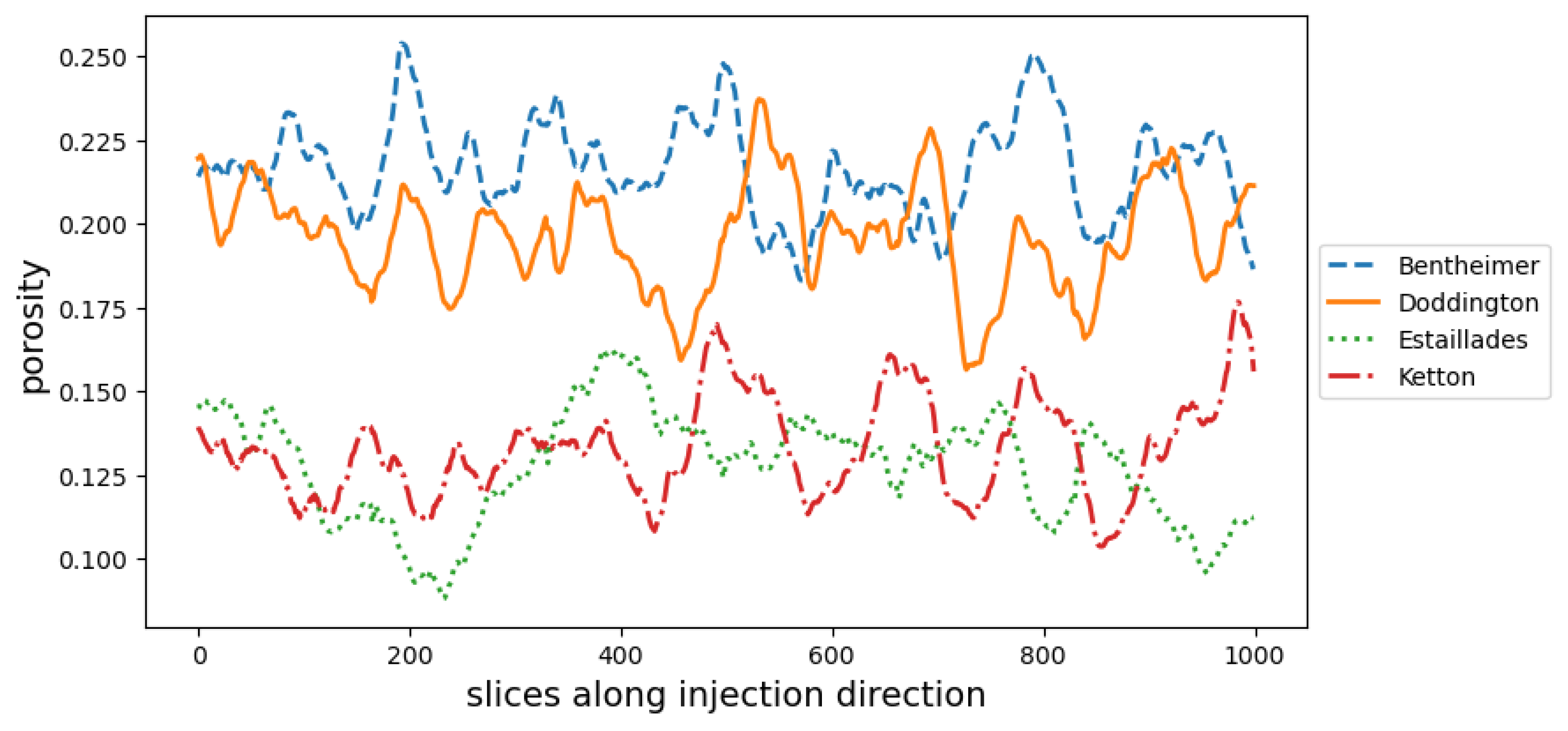
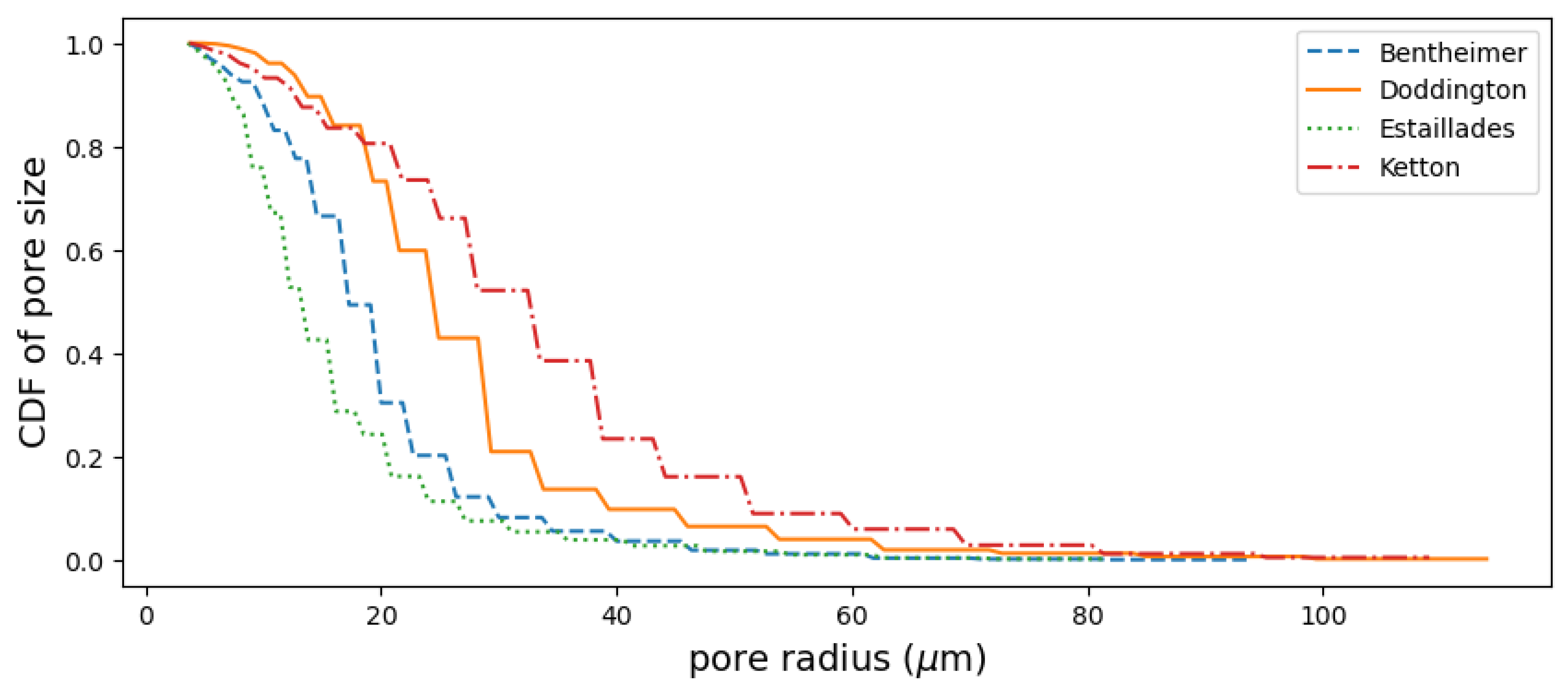
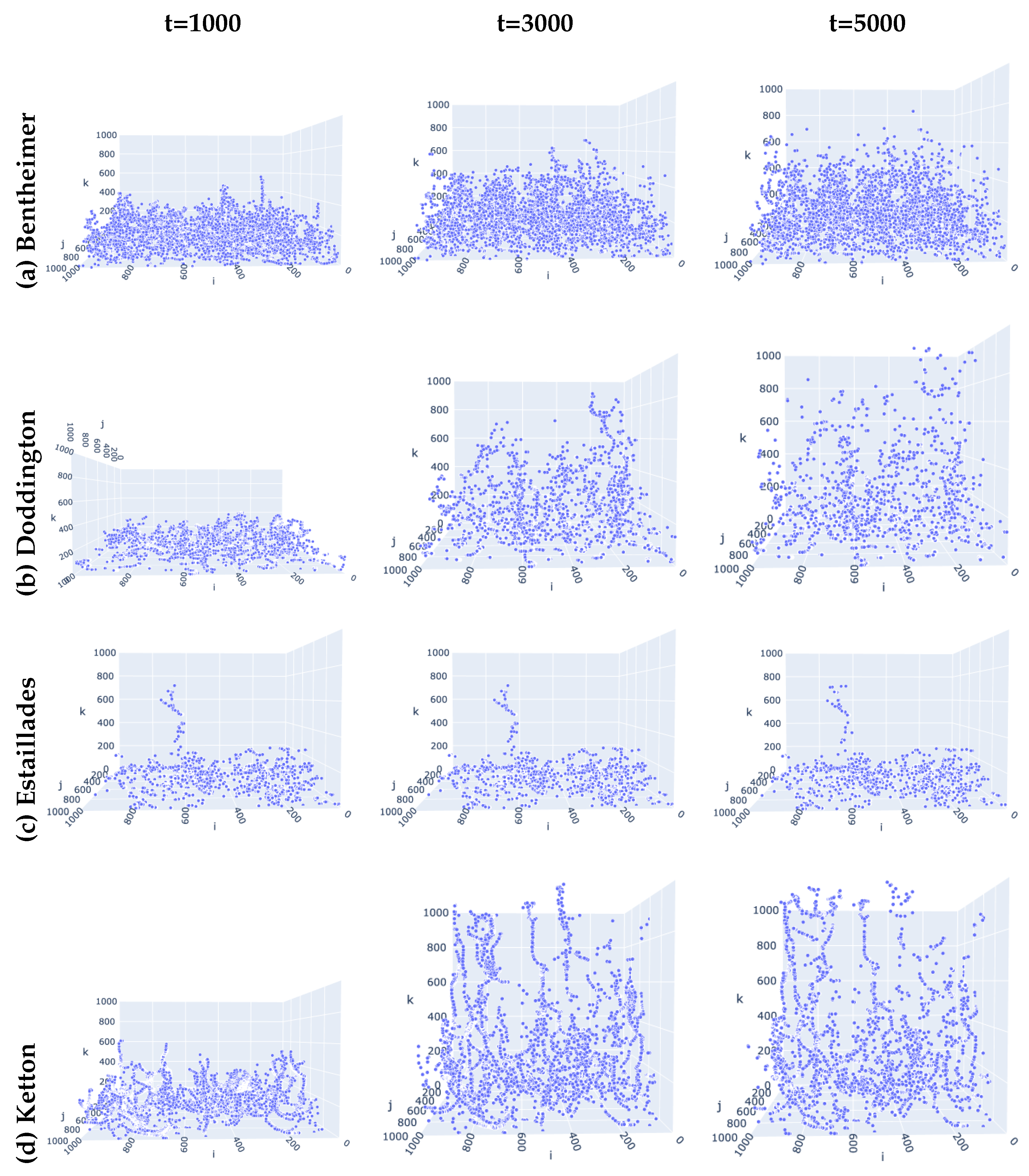
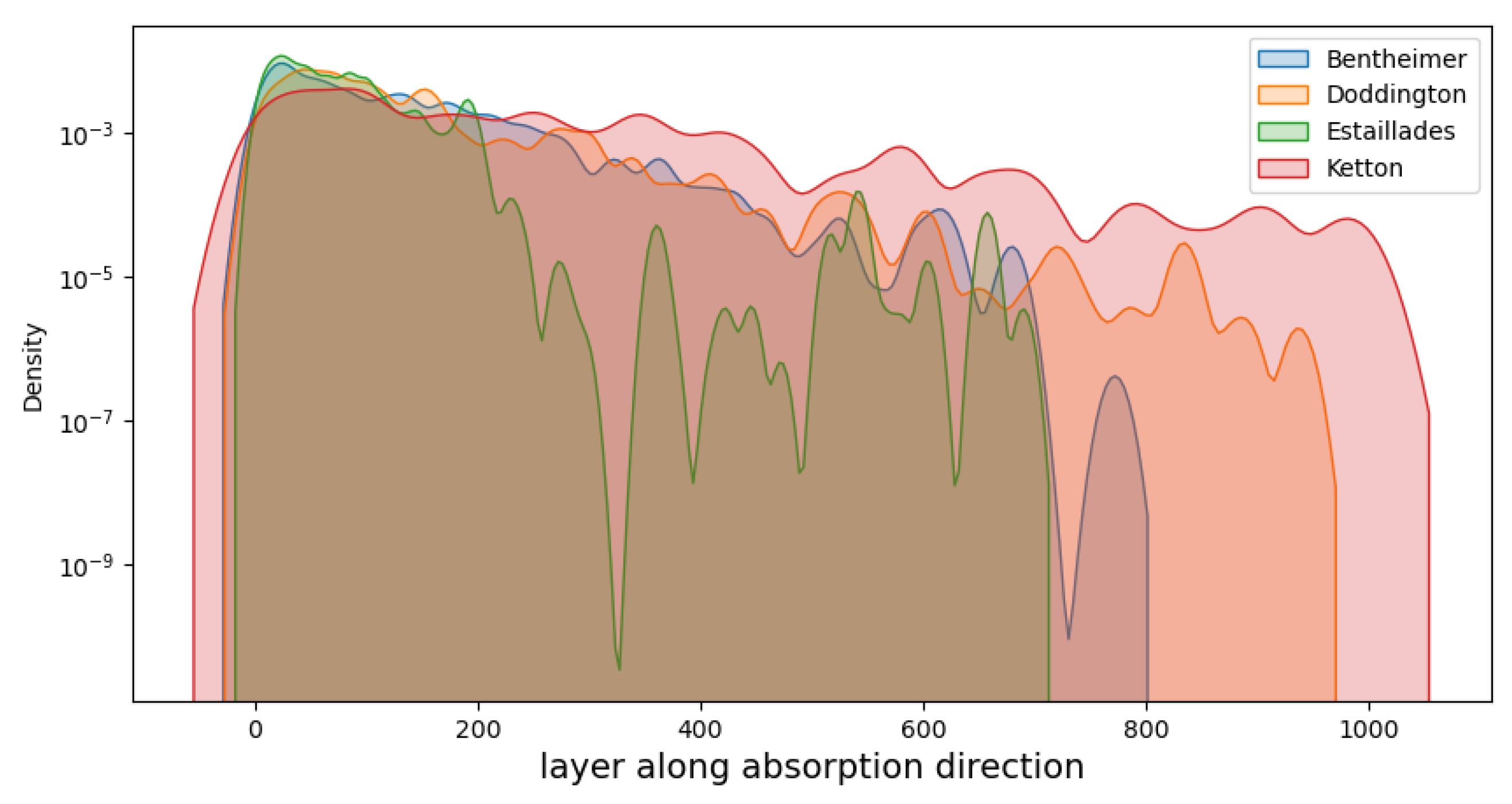
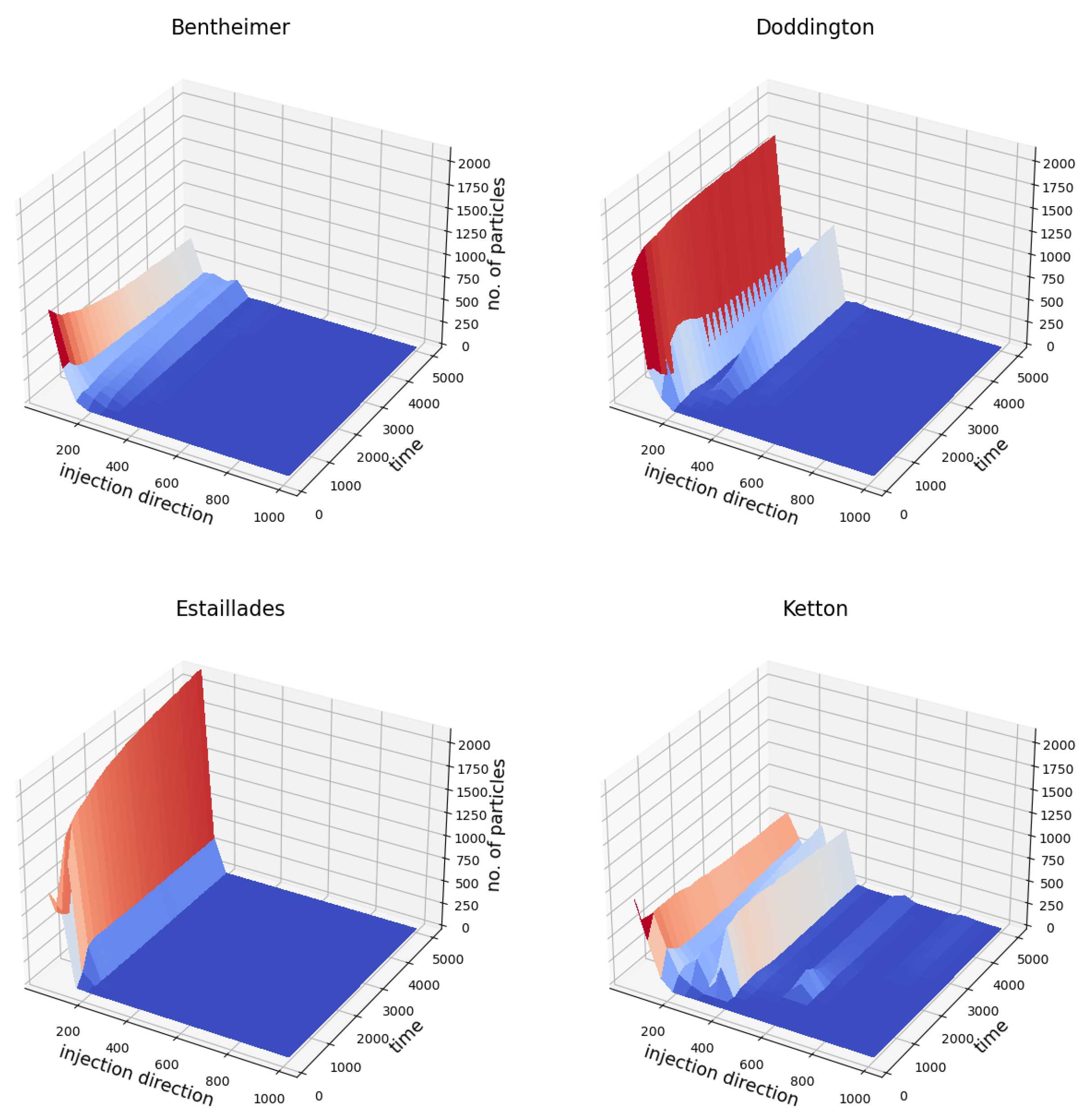
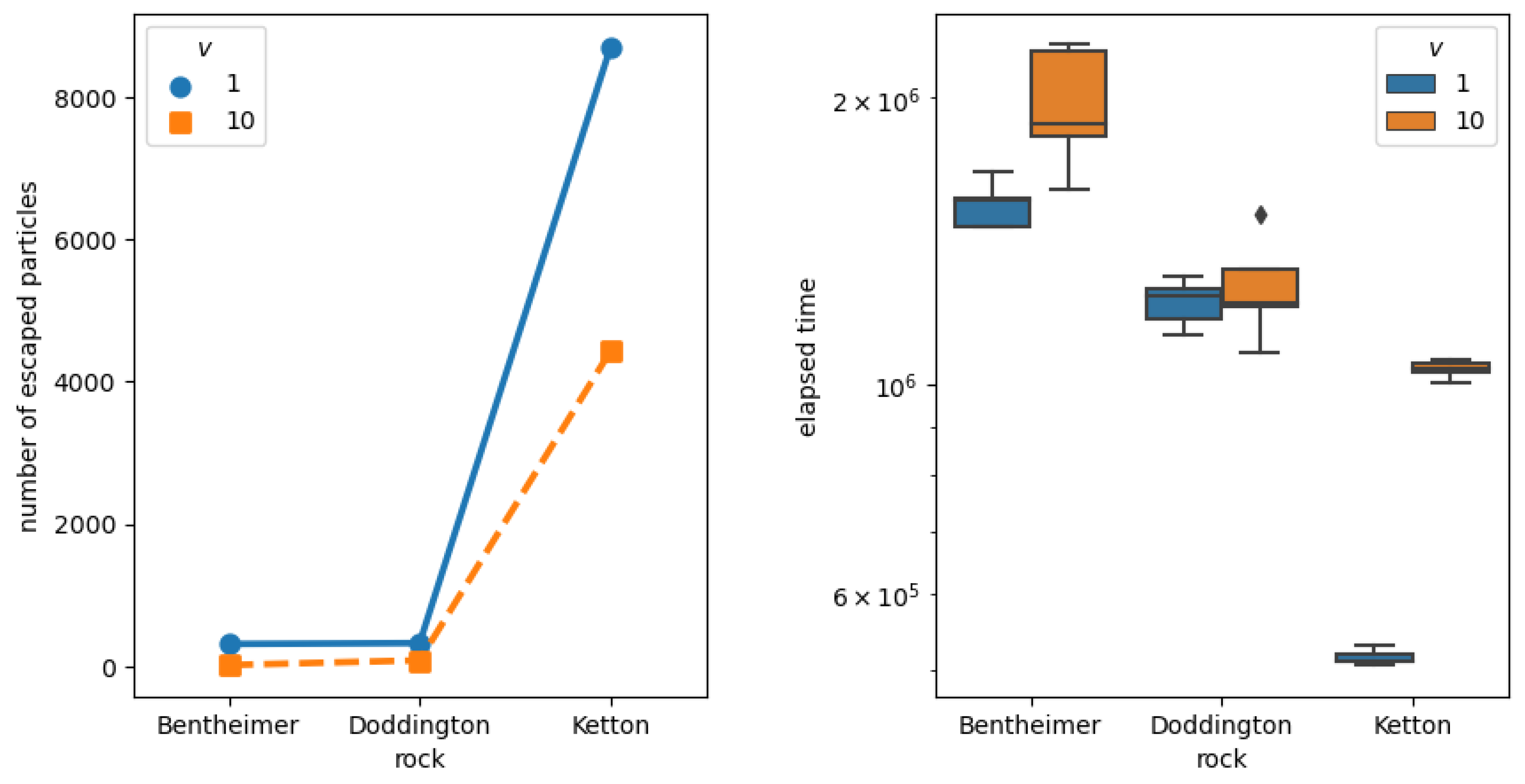
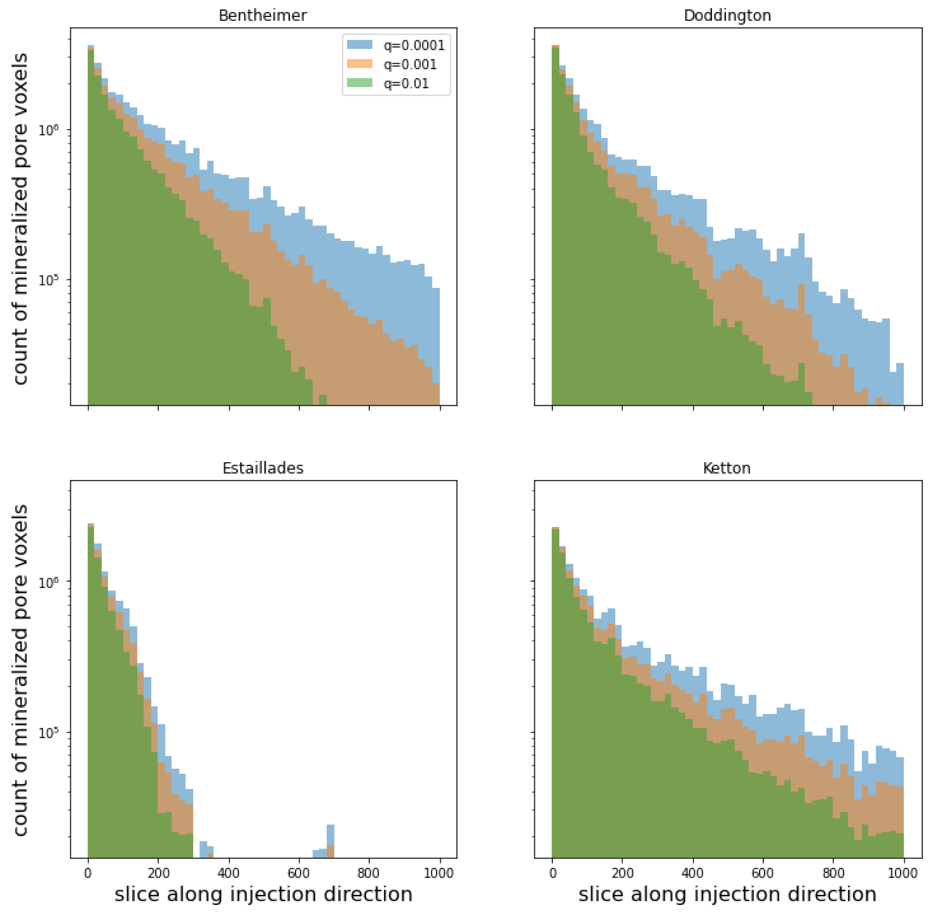
The time domain random walk method is applied to describe the movement of particles within complex, highly disordered, and heterogeneous pore spaces of porous rock formations under the pressure gradient imposed between the inlet and the outlet surfaces. The scheme is explicit and can be easily upscaled for large volumes of porous media samples. Based on numerical simulations, we investigated the particle fluid flow dynamics in four different types of natural porous rocks: Bentheimer, Doddington, Estaillades, and Ketton. The particle fluid flow dynamics were strongly affected by the geometric structure of the rocks. Ketton had the highest permeability among the four samples, despite having the lowest porosity.

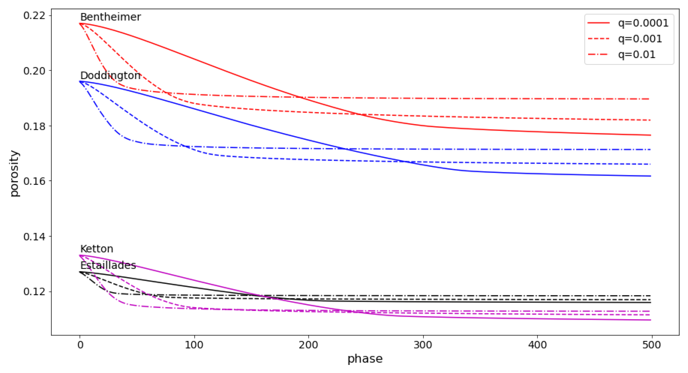
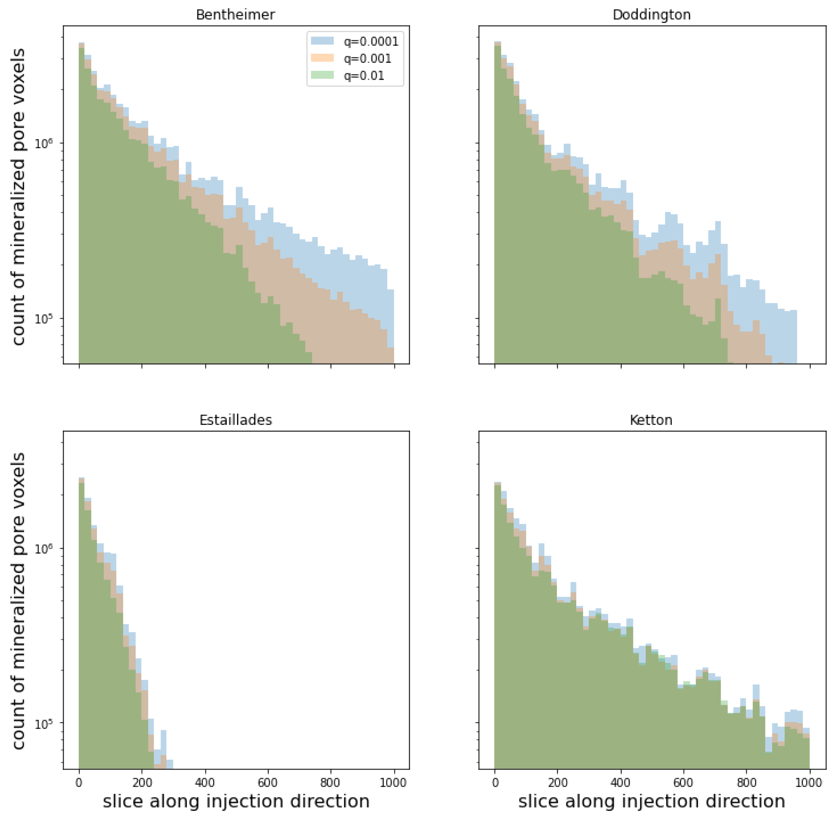
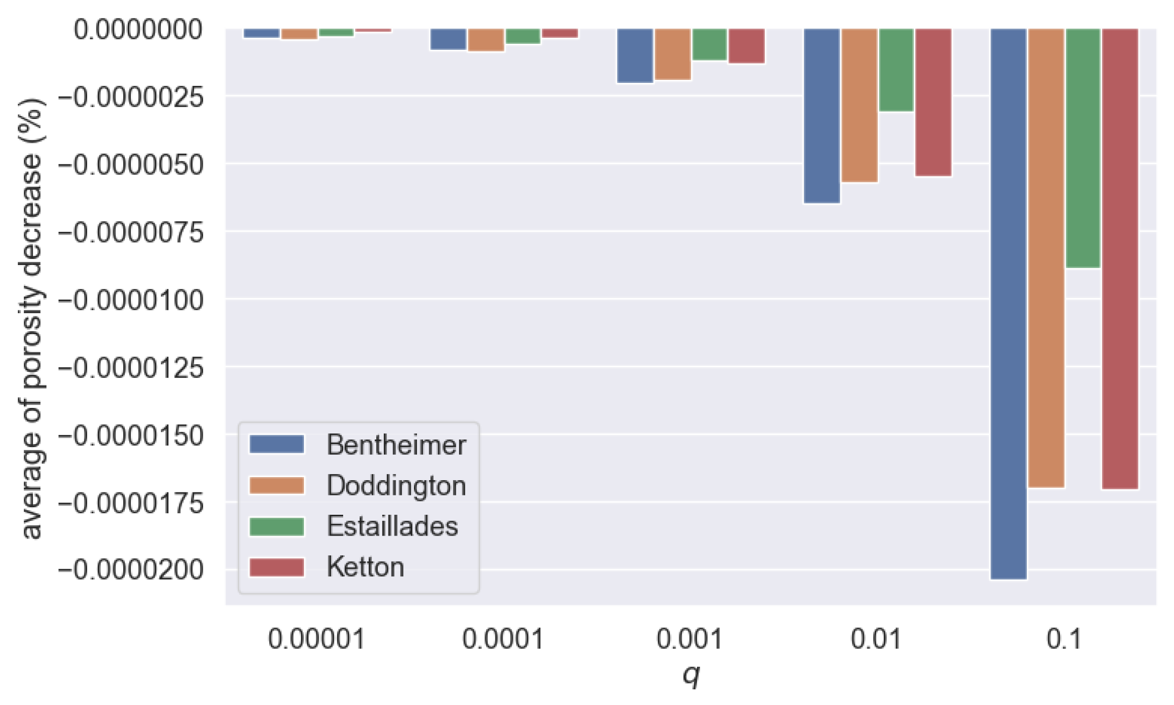
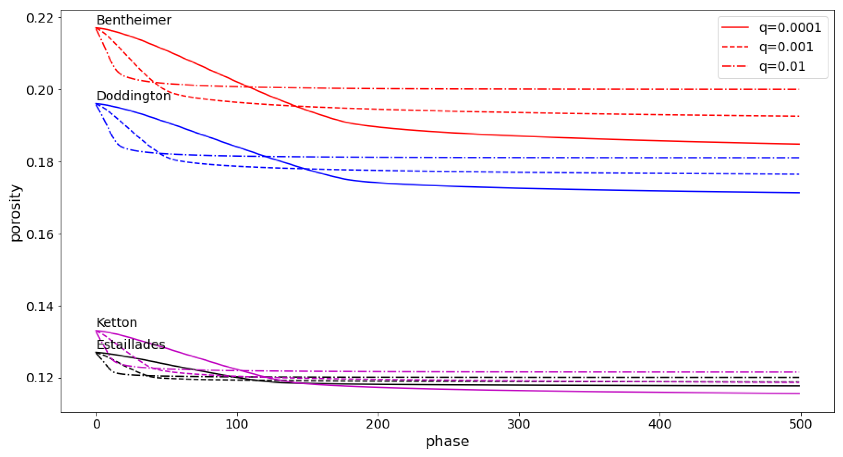
Based on the particle transport algorithm, we propose a probabilistic clogging model in two strategies: single- and multi-phase clogging. In the former strategy, the porosity decrease can be approximated as a monotonically non-increasing function of the deposition probability in the form of exponential functions. This monotonicity is no longer valid in the latter strategy, because the geometric structure changes at every phase. When some large probability of deposition is chosen, the fast clogging narrows the capillaries, preventing the particles from invading easily in the injection direction. Our simulation results suggest that Bentheimer, Doddington, and Ketton could potentially be used as rock formations for carbon dioxide storage, while Estaillades could not. The method proposed in this study could be useful in lithology selection for geological sequestration.

The simulation study revealed that the velocity v and deposition probability q are critical parameters that characterize the efficiency of the clogging process. While v models the pressure gradient imposed between the inlet and the outlet surface, q models the speed of chemical reactions between CO₂ and alkaline earth metals. Fine-tuning these factors helps increase the efficiency of geological sequestration technology, and the optimal values can be obtained from the simulation studies.

Once the target lithology has been chosen, the next step is to elucidate these formations’ trapping mechanisms. Mahmood et al. [39] utilized the kinetic Monte Carlo method to model the carbonation front development in calcium–silicate–hydrate microstructures under varying temperatures and then combine the simulation data with experimental results from Fourier-transform infrared spectroscopy (FTIR) and impedance spectroscopy, so as to provide insights into the carbonation process at different depths and temperatures. Learning from Mahmood et al.’s idea, in our future work we will incorporate the kinetic barrier of the chemical processes during the mineralized process, to define the rate constant; that is, the state-to-state transition rates in the RW algorithm through Arrhenius formulas. The simulation results will then be combined with atomic simulation and experimental data to help understand the complicated trapping mechanisms in the chosen lithology. Another important issue that needs to be addressed is the modeling of fracture systems. It is critical to access the risk of injected CO₂ leakage due to natural fault or fractures as well as the presence of abandoned oil/gas wells. This problem involves both fluid flow through aquifers and intensive fluid flow through fractures simultaneously. A hybrid approach incorporating the random walk model with a continuum has the potential to solving this challenging problem. For more details about the importance and challenges of this issue, as well as current numerical methods to solve these systems, we refer the interested reader to [40,41].

References

- Muhammad, A.; Nilesh, K.J.; Nilanjan, P.; Alireza, K.; Hussein, H.; Mohammad, S. Recent advances in carbon dioxide geological storage, experimental procedures, influencing parameters, and future outlook. Earth-Sci. Rev. 2022, 225, 103895. [Google Scholar]
- Metz, B.; Davidson, O.; De Coninck, H.C.; Loos, M.; Mayer, L. IPCC Special Report on Carbon Dioxide Capture and Storage; Cambridge University Press: New York, NY, USA, 2005. [Google Scholar]
- Krevor, S.; Blunt, M.J.; Benson, S.M.; Pentl, C.H.; Reynolds, C.; Al-Menhali, A.; Niu, B. Capillary trapping for geologic carbon dioxide storage—From pore scale physics to field scale implications. Int. J. Greenh. Gas Control. 2015, 40, 221–237. [Google Scholar] [CrossRef]
- Li, W.; Nan, Y.; Zhang, Z.; You, Q.; Jin, Z. Hydrophilicity/hydrophobicity driven CO2 solubility in kaolinite nanopores in relation to carbon sequestration. Chem. Eng. J. 2020, 398, 125499. [Google Scholar] [CrossRef]
- Smit, B.; Reimer, J.A.; Oldenburg, C.M.; Bourg, I.C. Introduction to Carbon Capture and Sequestration; Imperial College Press: London, UK, 2014. [Google Scholar]
- Jiang, F.; Tsuji, T. Changes in pore geometry and relative permeability caused by carbonate precipitation in porous media. Phys. Rev. E 2014, 90, 053306. [Google Scholar] [CrossRef]
- Niu, B.; Al-Menhali, A.; Krevor, S. A study of residual carbon dioxide trapping in sand-stone. Energy Procedia 2014, 63, 5522–5529. [Google Scholar] [CrossRef]
- Tanino, Y.; Blunt, M.J. Capillary trapping in sandstones and carbonates: Dependence on pore structure. Water Resour. Res. 2012, 48, 08525. [Google Scholar] [CrossRef]
- Al-Raoush, R.I. Impact of wettability on pore-scale characteristics of residual nonaqueous phase liquids. Environ. Sci. Technol. 2009, 43, 4796–4801. [Google Scholar] [CrossRef] [PubMed]
- Goodarzi, S.; Zhang, Y.; Foroughi, S.; Bijeljic, B.; Blunt, M.J. Trapping, hysteresis and Ostwald ripening in hydrogen storage: A pore-scale imaging study. Int. J. Hydrogen Energy 2024, 56, 1139–1151. [Google Scholar] [CrossRef]
- Selem, A.M.; Agenet, N.; Foroughi, S.; Blunt, M.J.; Bijeljic, B. Pore-Scale imaging of emulsification of oil during tertiary and secondary low salinity waterflooding in a reservoir carbonate. Energy Fuels 2023, 21, 16368–16377. [Google Scholar] [CrossRef]
- Zhang, Y.; Lin, Q.; Raeini, A.Q.; Onaka, Y.; Iwama, H.; Takabayashi, K.; Blunt, M.J.; Bijeljic, B. Pore-scale imaging of asphaltene deposition with permeability reduction and wettability alteration. Fuel 2022, 315, 123202. [Google Scholar] [CrossRef]
- Jiang, F.; Tsuji, T.; Hu, C. Elucidating the role of interfacial tension for hydrological properties of two-phase flow in natural sandstone by an improved lattice Boltzmann method. Transp. Porous Med. 2014, 104, 205–229. [Google Scholar] [CrossRef]
- Ahrenholz, B.; Tölke, J.; Krafczyk, M. Lattice Boltzmann flow simulations in reconstructed porous media. Int. J. Comput. Fluid Dyn. 2006, 20, 369–377. [Google Scholar] [CrossRef]
- Raeini, A.Q.; Blunt, M.J.; Bijeljic, B. Direct simulations of two-phase flow on micro CT images of porous media and upscaling of pore-scale forces. Adv. Water Resour. 2014, 74, 116–126. [Google Scholar] [CrossRef]
- Ferziger, J.H.; Peric, M. Computational Methods for Fluid Dynamics; Springer: Berlin/Heidelberg, Germany, 2002. [Google Scholar]
- Gentry, R.A.; Martin, R.E.; Daly, B.J. An Eulerian differencing method for unsteady compressible flow problems. J. Comput. Phys. 1966, 1, 87–118. [Google Scholar] [CrossRef]
- Chen, S.; Doolen, G.D. Lattice Boltzmann method for fluid flows. Annu. Rev. Fluid Mech. 1998, 30, 329–364. [Google Scholar] [CrossRef]
- Boek, E.S.; Venturoli, M. Lattice-Boltzmann studies of fluid flow in porous media with realistic rock geometries. Comput. Math. Appl. 2010, 59, 2305–2314. [Google Scholar] [CrossRef]
- Ramstad, T.; Idowu, N.; Nardi, C.; Øren, P.E. Relative permeability calculations from two-phase flow simulations directly on digital images of porous rocks. Transp. Porous Media 2012, 94, 487–504. [Google Scholar] [CrossRef]
- Ahrenholz, B.; Tölke, J.; Lehmann, P.; Peters, A.; Kaestner, A.; Krafczyk, M.; Durner, W. Prediction of capillary hysteresis in a porous material using lattice-boltzmann methods and comparison to experimental data and a morphological pore network model. Adv. Water Resour. 2008, 31, 1151–1173. [Google Scholar] [CrossRef]
- Pan, C.; Hilpert, M.; Miller, C.T. Lattice Boltzmann simulation of two-phase flow in porous media. Water Resour. Res. 2004, 40. [Google Scholar] [CrossRef]
- Tsuji, T.; Jiang, F.; Suzuki, A.; Shirai, T. Mathematical modeling of rock pore geometry and mineralization: Applications of persistent homology and random walk. In Agriculture as a Metaphor for Creativity in All Human Endeavors; Mathematics for Industry; Springer: Singapore, 2018; Volume 28, pp. 95–109. [Google Scholar]
- Tsuji, T.; Jiang, F.; Christensen, K.T. Characterization of immiscible fluid displacement processes with various capillary numbers and viscosity ratio in 3D natural sandstone. Adv. Water Resour. 2016, 95, 3–15. [Google Scholar] [CrossRef]
- Harris, C.R.; Millman, K.J.; van der Walt, S.J.; Gommers, R.; Virtanen, P.; Cournapeau, D.; Wieser, E.; Taylor, J.; Berg, S.; Smith, N.J.; et al. Array programming with NumPy. Nature 2020, 585, 357–362. [Google Scholar] [CrossRef] [PubMed]
- Virtanen, P.; Gommers, R.; Oliphant, T.E.; Haberl, M.; Reddy, T.; Cournapeau, D.; Burovski, E.; Peterson, P.; Weckesser, W.; Bright, J.; et al. SciPy 1.0: Fundamental Algorithms for Scientific Computing in Python. Nat. Methods 2020, 17, 261–272. [Google Scholar] [CrossRef] [PubMed]
- Hunter, J.D. Matplotlib: A 2D Graphics Environment. Comput. Sci. Eng. 2007, 9, 90–95. [Google Scholar] [CrossRef]
- Gostick, J.; Khan, Z.A.; Tranter, T.G.; Kok, M.D.R.; Agnaou, M.; Sadeghi, M.A.; Jervis, R. PoreSpy: A Python Toolkit for Quantitative Analysis of Porous Media Images. J. Open Source Softw. 2019, 4, 1296. [Google Scholar] [CrossRef]
- Alyafei, N.; Mckay, T.J.; Solling, T.I. Characterization of petrophysical properties using pore-network and lattice-boltzmann modeling: Choice of method and image sub-volume size. J. Pet. Sci. Eng. 2016, 145, 256–265. [Google Scholar] [CrossRef]
- Kinzelback, W. The random walk method in pollutant transport simulation. In Advances in Analytical and Numerical Groundwater Flow and Quality Modeling C; Custodio, E., Ed.; Springer: Dordrecht, The Netherlands, 1987; Volume 224, pp. 227–246. [Google Scholar]
- Salmon, P.; Fernandez-Garcia, D.; Gomez-Hernndez, J.J. A review and numerical assessment of the random walk particle tracking method. J. Contam. Hydrol. 2006, 87, 277–305. [Google Scholar] [CrossRef]
- Banton, O.; Delay, F.; Pore, G. A new time domain random walk method for solute transport in 1-d heterogeneous media. Ground Water 1997, 35, 1008–1013. [Google Scholar] [CrossRef]
- Noetinger, B.; Estebenet, T. Up-scaling of double porosity fractured media using continuous-time random walks methods. Transport. Porous Media 2000, 39, 315–337. [Google Scholar] [CrossRef]
- Delay, F.; Pore, G.; Sardini, P. Modeling diffusion in a heterogeneous rock matrix with a time-domain lagrangian method and an inversion procedure. Comptes Rendus Geosci. 2002, 334, 967–973. [Google Scholar] [CrossRef]
- Dentz, M.; Gauze, P.; Russian, A.; Dwell, J.; Delay, F. Diffusion and trapping in heterogeneous media: An inhomogeneous continuous time random walk approach. Adv. Water Resour. 2012, 49, 13–22. [Google Scholar] [CrossRef]
- Hostomski, J.; Jones, A.G. Calcium carbonate crystallization, agglomeration and form during continuous precipitation from solution. J. Phys. D Appl. Phys. 1991, 24, 165. [Google Scholar] [CrossRef]
- Shiraki, R.; Brantley, S.L. Kinetics of near-equilibrium calcite precipitation at 100 °C: An evaluation of elementary-reaction based and affinity-based rate laws. Geochim. Cosmochim. Acta 1995, 59, 1457–1471. [Google Scholar] [CrossRef]
- Keehm, Y.; Mukerji, T.; Nur, A. Computational rock physics at the pore scale: Trans-port properties and diagenesis in realistic pore geometries. Lead. Edge 2001, 20, 180–183. [Google Scholar] [CrossRef]
- Mahmood, A.; Ibuk, A.; Vogel, M.; Neuhaus, C.; Dehn, F.; Thissen, P. Unraveling carbonation and CO2 capture in Calcium-Silicate-Hydrate. ACS Sustain. Chem. Eng. 2023, 11, 13002–13012. [Google Scholar] [CrossRef]
- Wang, L.; Wang, Y.; Vuik, C.; Hajibeygi, H. Accurate modeling and simulation of seepage in 3D heterogeneous fractured porous media with complex structures. Comput. Geotech. 2022, 150, 104923. [Google Scholar] [CrossRef]
- Karimi-Fard, M.; Durlofsky, L.J. A general gridding, discretization, and coarsening methodology for modeling flow in porous formations with discrete geological features. Adv. Water Resour. 2016, 96, 354–372. [Google Scholar] [CrossRef]
Disclaimer/Publisher’s Note: The statements, opinions and data contained in all publications are solely those of the individual author(s) and contributor(s) and not of MDPI and/or the editor(s). MDPI and/or the editor(s) disclaim responsibility for any injury to people or property resulting from any ideas, methods, instructions or products referred to in the content. |
© 2025 by the authors. Licensee MDPI, Basel, Switzerland. This article is an open access article distributed under the terms and conditions of the Creative Commons Attribution (CC BY) license (https://creativecommons.org/licenses/by/4.0/).