Article

Comprehensive Forensic Tool for Crime Scene and Traffic Accident 3D Reconstruction

by
Alejandra Ospina-Bohórquez
1,*,
Esteban Ruiz de Oña
1,
Roy Yali
1,
Emmanouil Patsiouras
2,
Katerina Margariti
3 and
Diego González-Aguilera
1,*
1
Department of Cartographic and Land Engineering, Higher Polytechnic School of Ávila, Universidad de Salamanca, Hornos Caleros, 50, 05003 Ávila, Spain
2
Centre for Research and Technology Hellas, Information Technologies Institute, 57001 Thessaloniki, Greece
3
CERIDES, European University Cyprus, Nicosia 1516, Cyprus
*
Authors to whom correspondence should be addressed.
Algorithms 2025, 18(11), 707; https://doi.org/10.3390/a18110707 (registering DOI)
Submission received: 19 September 2025 / Revised: 27 October 2025 / Accepted: 4 November 2025 / Published: 7 November 2025
(This article belongs to the Special Issue Modern Algorithms for Image Processing and Computer Vision)

Abstract

This article presents a comprehensive forensic tool for crime scene and traffic accident investigations, integrating advanced 3D reconstruction and semantic and dynamic analyses; the tool facilitates the accurate documentation and preservation of crime scenes through photogrammetric techniques, producing detailed 3D models based on images or video captured under specified protocols. The system includes modules for semantic analysis, enabling object detection and classification in 3D point clouds and 2D images. By employing machine learning methods such as the Random Forest model for point cloud classification and the YOLOv8 architecture for object detection, the tool enhances the accuracy and reliability of forensic analysis. Furthermore, a dynamic analysis module supports ballistic trajectory calculations for crime scene investigations and the vehicle impact speed estimation using the Equivalent Barrier Speed (EBS) model for traffic accidents. These capabilities are integrated into a single, user-friendly platform offering significant improvements over existing forensic tools, which often focus on singular tasks and require expertise. This tool provides a robust, accessible solution for law enforcement agencies, enabling more efficient and precise forensic investigations across different scenarios.

1. Introduction

Car accidents and crime scenes have always been very complex scenarios, with numerous parameters that security forces organizations must consider to carry out accurate and thorough investigations. Over time, different tools emerged to ease the burden on the investigators. Still, it remains a tedious and complicated task that inspectors carry out precisely and rigorously since the results can have serious legal repercussions.
This paper presents a tool that pretends to become a powerful application to support car accident and crime investigation throughout the entire procedure. This tool combines state-of-the-art technology with forensic science to reconstruct 3D scenarios of crime and traffic accidents using photos or videos.
The tool was developed within the framework of the European LAW-GAME project, which focuses on virtual reality-based simulation and training for forensic scenarios. It serves as a complementary component to the training platform: once users complete training (particularly the image acquisition procedures) they can use this tool to verify whether the captured images are suitable for generating accurate 3D reconstructions. Furthermore, trained users can apply these protocols in real-world scenarios, producing 3D models that, in turn, can be used to generate new simulated environments for further training. To the best of our knowledge, no existing tool enables this bidirectional workflow, bridging real-world scene capture and simulation, while simultaneously supporting both traffic accident and crime scene domains, where environmental preservation is critical for effective investigation.
The main objective of this tool is to recreate 3D scenarios with metric information: it converts 2D photographic data or videos into immersive and detailed 3D environments of crime scenes and traffic accidents. The tool provides a visual and interactive platform for reconstructing scenarios, allowing the users to return to the location to retrieve new information.
The tool scope is expansive: in addition to the scene preservation over time through its 3D reconstruction, the tool has different modules that, among other things, allow it to perform ballistic analysis for crime scenes and impact speed analysis for traffic accident scenarios. The first step to achieve any forensic investigation is to carry out a visual inspection; to this end, the tool includes a semantic analysis module that supports the semantic classification of the scene both in 2D based on the photographs used for the reconstruction, and in 3D on the generated point cloud.
Also, the tool has a dynamic analysis module that exploits algorithms and computational models to provide detailed data about projectile paths, impact speeds and other relevant forensic aspects to support investigators and analysts by providing them with comprehensive insights. All its modules are within an intuitive interface that adapts to various forensic domains. To validate this user-friendly design, several usability tests were conducted throughout the LAW-GAME project with end-users from law enforcement and forensic backgrounds. One of the key evaluation questions was: “Please rate the overall Standalone tool by taking into account the user friendliness of the application, the time needed to recreate the 3D, errors, etc.” Participants rated the tool on a scale from 1 to 10. For the traffic accident scenario, the average score was 8.0, while for the crime scene scenario, the score was 8.10. These results substantiate the claim that the tool is accessible and effective for non-expert users.
The tool encompasses the following:
  • Photo or video-based 3D reconstruction: the tool recreates detailed 3D environments with metric capabilities from photographic evidence, employing cutting-edge image processing and computer vision techniques.
  • Semantic 2D/3D analysis module: the tool includes a module for the semantic classification of the scene in 2D (based on photographs) and 3D (based on the 3D point clouds generated).
  • Forensic analysis modules: the tool includes tailored modules focused on ballistics and car impact speeds. It offers an analysis and visual representation of bullet trajectories and collision dynamics.
  • Intuitive user interface: a user-friendly interface allows easy navigation and utilization for forensic investigators and analysts.
  • Applicability: the tool was designed for security and law forces organizations, forensic experts, and other professionals involved in forensic investigations. It serves as a resource for comprehensive scene analysis.

1.1. State of the Art

This section aims to highlight the main contributions within the Scientific Community related to the 3D digitization of crime scenes and traffic accidents, as well as their forensic analysis. Likewise, it is intended to review the main existing tools on the market that focus on these tasks.

1.1.1. Forensic 3D Digitisation and Analysis Methods

Forensic scenario preservation is a crucial step in conducting correct and in-depth investigations, which has led to the development of forensic infographics, a technique that facilitates the virtual reconstruction of different events through computer science and digital image management.
Currently, innovative infographic techniques are applied for visual inspection of forensic investigations. These techniques encompass exhaustive observation and documentation tasks to obtain information that allows associations between all signs to determine and demonstrate facts [1]. However, its role within investigations has been relegated to supporting research and visual analysis for years.
In recent times, the forensic infographics domain has been incorporating geomatic and non-intrusive techniques based on the remote acquisition of information, allowing the scene to remain intact without any alteration of its position or its physical properties. Furthermore, the remote acquisition of information provides the metric recreation of the incidents in a rigorous, exhaustive and precise manner, allowing to return to the crime scene to reconstruct the facts. In this regard, the most used geomatic techniques are laser scanning [2,3,4,5] and close-range photogrammetry [6,7,8], permitting dimensional analysis and 3D reconstruction of scenarios. Also, these two methods are applied together to complement each other [9]. Laser scanning methods are applied in scenarios with objects with complex shapes and deficient illumination conditions where it is difficult to model using photogrammetry methods [10,11,12]; however, in some cases, it is impossible to apply these techniques due to their high costs and the complications related to mobility and layouts in reduced scenes. Photogrammetry is a much more manageable and affordable technique mainly used in scenarios that are not very complex from a geomatic point of view; nevertheless, to apply photogrammetry methods, it is often necessary to calibrate to ensure high-quality results, which represents a barrier to inexperienced users.
To overcome the limitations remarked above, in recent times, photogrammetry has begun to be combined with computer vision techniques within tools [13,14] to obtain high-quality results even in complex scenarios. These tools have been used in different studies [15,16]. The most relevant difference and advantage of the tool presented in this article is the ability to reconstruct any scenario in 3D using multiple images taken with any type of camera, including smartphones and tablets.
The tool integrates computer vision and photogrammetry algorithms to overcome the complexity of 3D reconstruction of objects (i.e., victims, weapons, evidence, etc.) and complex scenarios (i.e., interior scenes with shadows and occlusions) typical of the forensic field. To address these complex scenarios, it uses the latest generation of algorithms for image matching and orientation; for the self-calibration process, it combines different lens calibration models and applies multiple stereo vision algorithms. The tool provides the end user (i.e., law enforcement) with a simple, automatic and inexpensive way to obtain a quality 3D reconstruction with metric capabilities of different forensic scenes.
At this point, it is relevant to highlight the new methods with artificial intelligence to create 3D models from photographs: the Neural Radiance Field [17]. This method applies machine learning, specifically, a multilayer perceptron, to recreate complex spaces using a set of photos. The input consists of continuous 5D coordinates (the spatial location (X, Y, Z) and viewing direction (θ, φ)), and its output is the view-dependent emitted radiation and volume density at that spatial location. This technique generates photorealistic views for scenes with complex geometries and appearances and offers models with smaller file sizes than traditional model formats [18]. It allows 3D reconstruction in ways that were not previously possible [19,20,21,22] and has been successfully tested for facial reconstructions [23] and traffic accidents [18]. However, this method highly sensitive to camera calibration errors, which can result in blurred reconstruction areas of the scene captured by improperly calibrated cameras.
On the other hand, traffic accidents are a leading cause of mortality in developed countries, making them a notable concern for security forces. The investigation that must be carried out when a traffic accident occurs can become very complex due to the large number of factors involved: regulatory, legal, medical, and physiological, among others; these factors in some cases impede the adequate evaluation of the scene [24]. However, this assessment is essential for security forces, administrations and those involved in the accident. Therefore, establishing accurate and reliable investigation strategies is primordial.
In many cases of traffic accidents, the principal cause is the speed of the vehicle, so one of the most critical factors when reconstructing an accident is the estimation of the velocity of the automobiles involved, allowing the evaluation of the driver’s responsibility in the accident. Nevertheless, the anti-lock braking system (ABS) nearly eliminates skid marks on the road, making the analysis of impact speed more challenging. To overcome this obstacle, security forces employ a technique that studies vehicle deformations and spatial displacements involved in the accident [25]. This technique requires acquiring precise measurements on both the scene and the automobiles.
The method for acquiring these measurements relies on manual and rudimentary processes using a measuring tape [26], resulting in a significant dependence on the users’ skills and the outcome. This procedure often leads to less accuracy and reliability than desired. It is crucial to highlight that these measurements cannot be repeated for verification, as the geometric characteristics of the road change once all research procedures have been completed. This fact makes the development of strategies that allow for a precise metric reconstruction of the accident essential so that it can be analysed at any time. Beyond that, this reconstruction must enable an energetic analysis of the accident, allowing for a dynamic analysis of the collision event.
In the case of photogrammetry, there are various studies featuring approaches to estimate vehicle deformation for specific purposes [27,28]. However, the correct application of the proposed methods requires using sophisticated sensors that need to be calibrated, as well as complex target systems [29] and knowledge of photogrammetry. In other studies [30,31], robust image orientation and self-calibration methods are explored, but they require coded targets that support the photogrammetric orientation process. Some authors have developed new algorithms for detecting coded targets [32]; however, these targets require optimal exposure to ensure success, so they only function accurately in controlled indoor environments. Recently, there have been studies that attempt to determine the impact speed by evaluating the crush volume using images [33]. In the laser scanners field, they can provide real-time 3D point clouds in absolute darkness or direct sunlight cases without requiring prior knowledge of photogrammetry. In some studies, data collected from laser scanners are used for 3D modelling of accidents, offering new ways to simulate the accident [34], but they do not have the capability for direct computation of the collision event dynamics. Other authors have worked with photogrammetry and laser scanning procedures for traffic accident analysis and scene reconstruction [35,36]. The results obtained regarding the quality of the 3D models are outstanding, as it is possible to examine the bodies internally and externally. However, one of the main disadvantages is the high cost of the sensor, as well as its availability to all law enforcement officers who would require it. Additionally, this method is slow in situations where time is critical.
These 3D models, derived from photogrammetry or laser scanning acquisitions, are valuable for their crime scene or traffic accident reconstruction ability for digital documentation and the relevant information extraction to clarify the facts surrounding the scene. The information of interest includes:
  • Pure geometric data (linear, angular, surface, or volume measurements).
  • Pure radiometric data (detection of fluids such as water, gasoline, and blood, among others)
  • A combination of both for the detection of relevant objects in the scene. This process is known as semantic information inference of the scene or the semantic classification of point clouds.
Different methods for point cloud classification can be found, such as those based on region and edge detection [37] or those focused on model fitting, which rely on the possibility of fitting geometric primitives to 3D shapes [38]. Additionally, some methods exploit the geometric and radiometric properties of point clouds [39], e.g., LiDAR provides a complete waveform for property extraction [40], spectral information within the property selection framework shows promising results and hierarchical properties exhibit superior performance [41]. Regarding classifiers, various artificial intelligence methods have been applied to achieve better results. Among the different machine learning approaches, random forest is also used for point cloud classification [42]. However, an increasingly popular approach relies on deep learning models for point cloud segmentation [43]. In 2016, deep learning permitted a significant advancement in this area with the release of PointNet [44], the first model capable of directly processing raw point clouds without needing additional 2D information or transformations. Since then, significant efforts have been made on reference datasets to improve results, such as in S3DIS [43,44,45,46,47,48]. In 2021, a new architecture, PointTransformer [45], was published. It is based on self-attention layers using a concept analogous to queries, keys, and values to enrich the input with contextual information. In the same vein, SuperPointTransformer was introduced in 2023, offering an architecture for large-scale 3D scene semantic classification. This method incorporates a fast algorithm that segments point clouds into hierarchical superpoint structures, significantly reducing preprocessing time [49].
This review allows the authors to conclude that modern photogrammetry faces new challenges and changes, to which the scientific community has responded with new algorithms and methodologies for the automatic processing of images. However, access to these solutions for non-expert users without a background in photogrammetry and their application in specific fields to support problem-solving and decision-making remains a complex issue.

1.1.2. Software and Tools for 3D Reconstruction

Image processing based on computer vision and photogrammetry algorithms integration has recently become a valuable and powerful approach for 3D reconstruction. In the early 2000s, attention and interest shifted from photogrammetry and computer vision to laser scanning technologies. Recently, the opposite trend has been observed, with image-based approaches becoming the focus of attention. These approaches ensure sufficient automation, low costs, efficient results, and ease of use even for non-expert users.
In the last decade, various studies have contributed to the workflow of image-based modelling, including image processing [50,51], key point extraction [52,53], bundle adjustment [54,55,56], and dense and accurate point cloud generation [57]. These advancements in the field have led to the establishment of the Structure from Motion (SfM) methodology, a methodology capable of processing large image datasets and generating 3D outputs: sparse and dense models. These outputs have a level of detail and accuracy that varies depending on the application [58,59,60,61]. However, this approach can be inefficient when working with close-range applications where geometric and radiometric requirements are critical, such as in crime scenes or traffic accidents. In these cases, the precision, accuracy, and reliability of the results fall short of the standards typically claimed by the photogrammetric community. Nevertheless, some recent studies [62,63] have presented significant advancements in 3D reconstruction, both in indoor and outdoor environments, that have provided good results regarding completeness and accuracy.
Within the photogrammetry community, open-source code exchange is not a common practice. However, educational tools have been developed, such as sv3DVision [64], which allows dimensional analysis of scenes in the fields of engineering and architecture; Arpenteur [65], for 3D reconstruction using only a single image; simulation and learning of image-based photogrammetry [66]; the PW-Photogrammetry Workbench [67]; and PhoX [68], which is a free software for autonomous learning that includes tests and exercises with real photogrammetric data.
Since 2005, Marc Pierrot-Deseilligny has developed the open-source MicMac tools [15]. These tools integrate various scientific developments for satellite, aerial, unmanned aerial vehicles (UAVs), and terrestrial photogrammetry to create digital elevation models (DEMs), dense point clouds, and orthoimages. However, the lack of a user-friendly graphical interface (GUI) for non-expert users poses a significant limitation.
For image-based 3D modelling, other free and open-source solutions include a user-friendly interface, such as VisualSFM [69], PMVS [70], Bundler [55], and Python Photogrammetry Toolbox [71], among others. However, these do not guarantee accurate and reliable results and lack georeferencing and spatial information procedures. Recent developments include tools like Open Drone Map (ODM) [72], MVE [73], Theia [74], COLMAP [56], GLOMAP [75], and Graphos [76]. ODM supports georeferencing by incorporating Ground Control Points (GCPs) in bundle adjustments. MVE (Multi-View Environment) enhances the Bundler SfM pipeline with multiple variations. Theia offers both incremental and global SfM pipelines with recent advancements. COLMAP, building on Bundler’s incremental SfM, incorporates additional verification, outlier filtering, and model selection techniques to enhance processing robustness. GLOMAP is a general-purpose global SfM pipeline designed to perform simultaneous estimation of both camera positions and 3D point locations. It achieves a comparable level of robustness and accuracy to other SfM methods, while preserving the computational efficiency typical of global SfM pipelines. Graphos is a photogrammetric platform designed for close-range applications, capable of handling the entire 3D image-processing pipeline. It also supports a wide range of sensor types, enabling versatile and comprehensive 3D reconstructions across different imaging setups.
Recent NeRF neural networks [17] offer an alternative to traditional photogrammetry by generating volumetric representations of scenes. NeRF excels in 3D reconstruction, particularly in challenging scenarios involving thin or reflective objects [77]. These networks are designed to produce high-resolution, photorealistic novel views. Additionally, 3D reconstructions can be derived from NeRF outputs using classical computer vision techniques. Thus, NeRF represents a promising and advancing approach in the 3D reconstruction field. In the same vein, 3D Gaussian Splatting [78] has recently emerged as a powerful technique in the fields of neural radiance and computer graphics. It is based on the introduction of three key elements to achieve high visual quality in results. (i) Starting from the sparse model obtained during camera calibration, the scene is represented with 3D Gaussians that preserve the properties of continuous volumetric radiance fields for scene optimization, avoiding calculations in empty spaces. (ii) A density control of the 3D Gaussians is performed, optimizing anisotropic covariance to achieve an accurate representation of the scene. (iii) It uses a fast-rendering algorithm that supports anisotropic splatting and accelerates both training and real-time rendering.
In forensic scene reconstruction, several commercial software tools are crucial for converting 2D crime scene images into detailed 3D models. Notable examples include iWitness [79], PhotoModeler [80], and Reality Capture [81]. These tools offer advanced functionalities beyond basic reconstruction, such as vehicle speed estimation, vehicle damage analysis, bullet trajectory examination, and crash scene reconstruction. Recon-3D [82], an iPhone app, enables real-time scene scanning and 3D modelling for smaller environments, but extended use (1–2 min) may lead to precision loss, and while cloud and Wi-Fi integration enhance performance, they reduce overall accuracy.
These software solutions often feature interactive tutorials, video guides, and case studies demonstrating their capabilities. Some also offer user forums for exchanging tips and troubleshooting advice. However, they generally lack specific tools for impact speed estimation or shooter position analysis.
In the realm of free software, tools such as 3DF Zephyr [83] (offering a free version for up to 50 images with limited export capabilities) and Meshroom [84] provide accessible entry points for 3D reconstruction. These tools employ photogrammetry and computer vision techniques, appropriate for basic visualization and educational purposes. They often include online training modules, interactive webinars, or virtual workshops to facilitate learning, and may feature gamified elements to enhance user engagement.
For scene analysis, specialized commercial software such as Trimble Forensics Reveal [85,86], Forensic Architecture [87], Elcovision [88] (integrated with AutoCAD), and dedicated ballistics tools address various forensic needs. These applications enable bloodstain shape measurement, provide specialized 3D models for different incidents, and facilitate ballistic trajectory calculations, thereby supporting the investigative process. They often feature visual case studies, interactive demonstrations, and 3D model samples that showcase their analytical capabilities in real and simulated crime scenes.
Considering the solutions discussed, the tool presented in this study offers a comprehensive photogrammetric and computer vision platform for crime scene reconstruction and car accident analysis. It performs all stages of the 3D image-processing pipeline and supports various sensors and image types (e.g., RGB, NIR, TIR).
The software presented was designed specifically for forensic applications, offering distinct advantages over commercial and free solutions. This specialized software provides a streamlined 3D reconstruction workflow with an intuitive interface and integrates functionalities for ballistic analysis, accident speed assessment, and scene element classification. It serves as a valuable training tool for law enforcement, featuring modules that simulate crime scenes and allow for practice in photogrammetric data collection. Unlike generic software, these forensic tools include specialized modules tailored to the unique needs of crime scene reconstruction and analysis, which are often lacking in more general commercial and free options.

2. Materials and Methods

This section describes the methods included in the tool development presented in this study.

2.1. System Architecture Overview

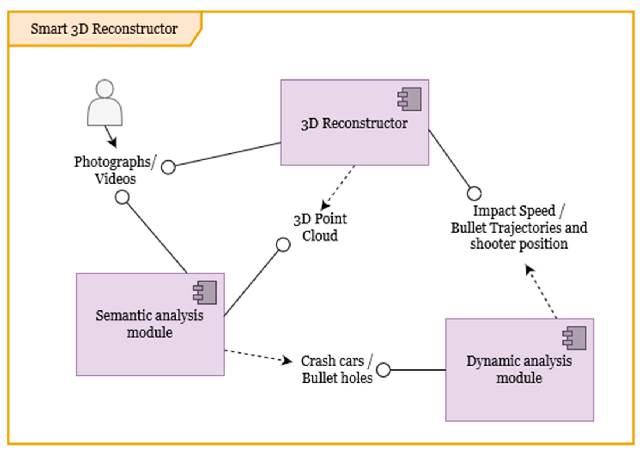
To provide a clearer understanding of the software’s structure and functionality, Figure 1 presents the system architecture, highlighting its core modules and their interactions.
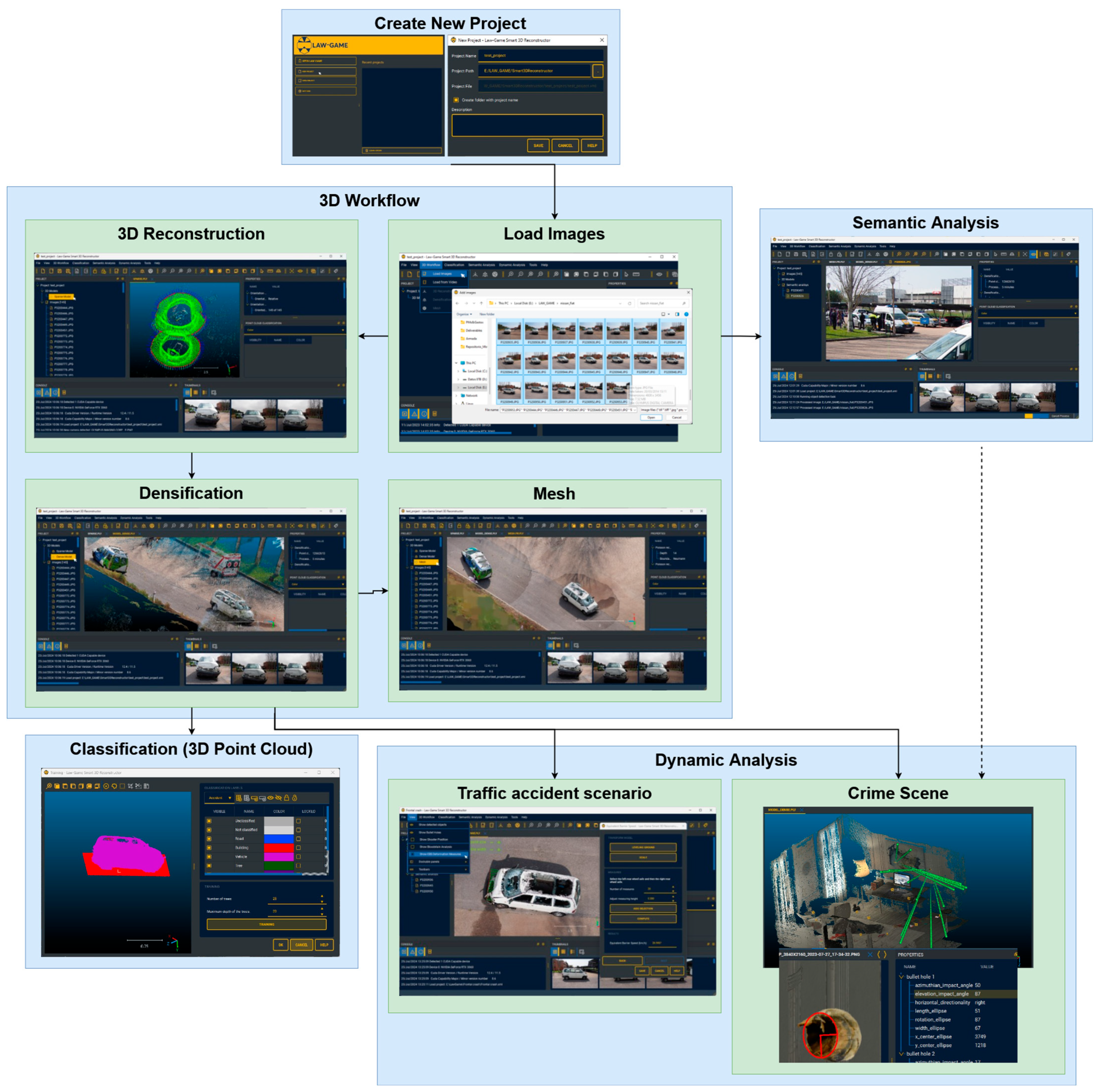
Figure 2 illustrates the user workflow, detailing the sequential steps involved in data acquisition, processing, analysis, and output generation.

2.2. Generation of Smart 3D Scenarios

The generation of smart 3D scenarios includes different stages described in this section: generation of 3D environments from images or videos, semantic and dynamic analyses. These three stages are included as components of the tool as shown in Figure 3.

2.2.1. From 2D Photographs/Videos to 3D Environments

Regarding the reconstruction of 3D environments, the tool presented in this article encapsulates different tasks (Figure 4): image data acquisition, feature extraction and matching, image orientation and self-calibration and dense matching.
Image data acquisition: The input data may include images or videos obtained through convergent or parallel protocols (Figure 5). For video input, the tool extracts individual frames to capture snapshots from various positions and orientations relative to the scene. While the tool allows users to define the desired frame rate, it does not implement automatic frame selection or discard mechanisms, users are responsible for supervising and curating the extracted frames. Additionally, the system applies automatic preprocessing to enhance image quality, including contrast adjustment, brightness normalization, and noise reduction:
  • Parallel Protocol: This protocol is optimal for detailed reconstructions of specific areas, such as vehicle deformations or crime scene features (e.g., bullet holes, footprints, bloodstains). The user should capture five images arranged in a cross pattern (Figure 5, left), with at least 80% overlap between images. The central image (red) should focus on the area of interest, while the four surrounding images (left, right, top, and bottom) should be taken with the camera angled towards the central area. Each image must cover the entire region of interest for a comprehensive reconstruction.
  • Convergent Protocol: This protocol is well-suited for reconstructing 360° 3D point clouds, such as those of accident scenes or entire crime scenes. The user should capture images while moving in a ring around the object, maintaining a constant distance and ensuring more than 80% overlap between images (Figure 5, right). If the object cannot be captured in a single ring, a similar approach using a half-ring can be employed.
Figure 5. Data acquisition protocols. (Left) Parallel Protocol. (Right) Convergent Protocol.
Algorithms 18 00707 g005
Feature extraction and matching are critical tasks in the 3D reconstruction process, as they provide the spatial and angular information necessary for image orientation and camera self-calibration. Crime scenes and traffic accidents often involve variations in scale and illumination that make classical algorithms like Area-Based Matching (ABM) [89] and Least Squares Matching (LSM) [90] ineffective. Advanced algorithms such as SUSAN (Smallest Univalue Segment Assimilating Nucleus) [91], MSER (Efficient Maximally Stable Extremal Region) [92], and SURF (Speeded Up Robust Features) [93] have been evaluated for their robustness under these conditions. However, these methods also struggle with significant scale and rotation differences between images.
In the same way, the authors tested two deep learning-based detectors/descriptors: D2-Net [94] and R2D2 [95], chosen for their high performance and availability as pre-trained models not restricted to specific datasets. Although they work well under unfavorable conditions (obtaining a higher density of matching points), the results presented for these cases were not comparable with the results from the classic detectors/descriptors because when performing the triangulation and beam adjustment, the solution did not converge.
Finally, for the feature extraction, it was decided to integrate into the developed method the SIFT (Scale Invariant Feature Transform) [96] algorithm, more specifically the SiftGPU library [97] if the machine where the tool is executed supports CUDA or the OpenCV SIFT [98] implementation if it does not.
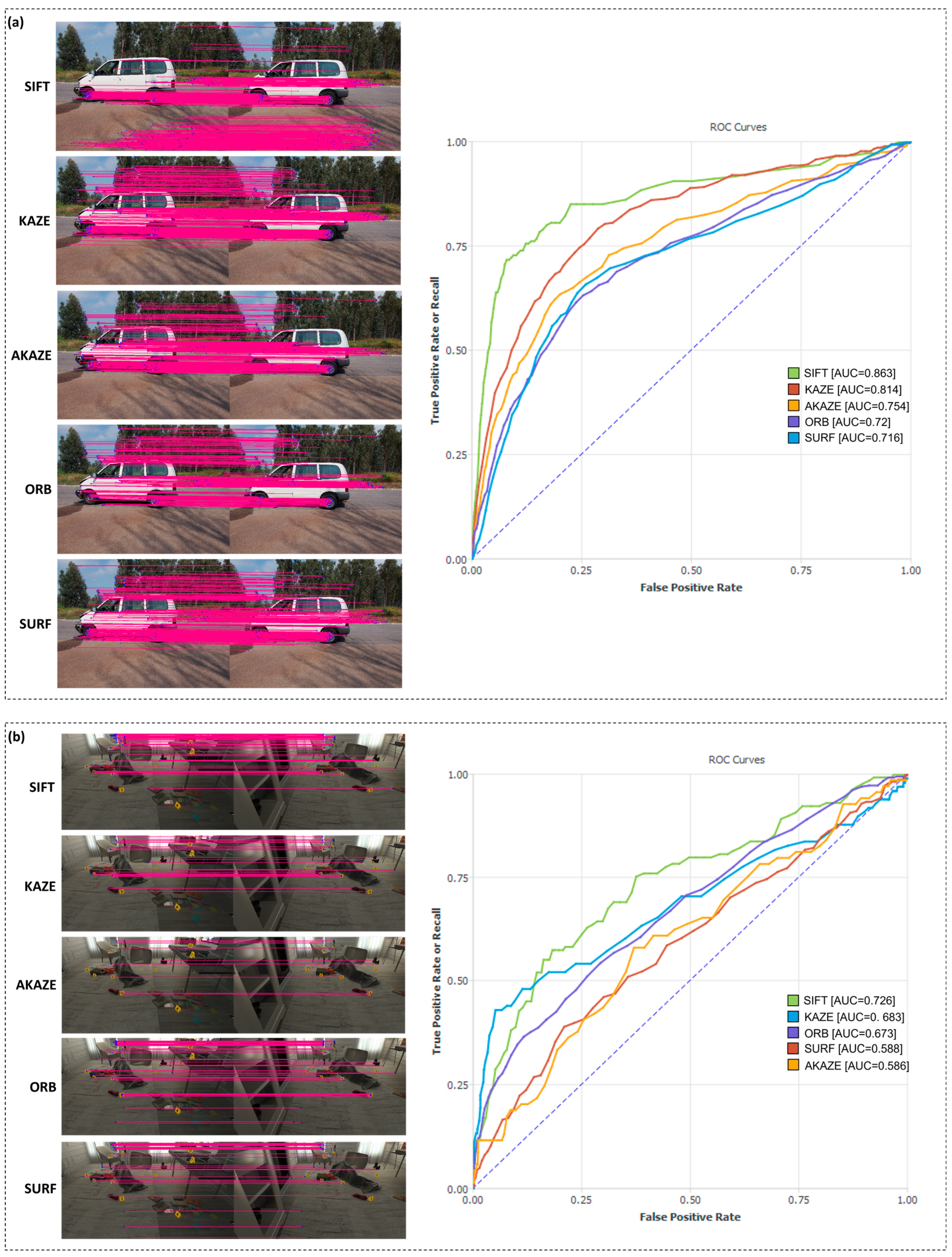
To support this decision, a comparative evaluation was conducted using five feature extraction algorithms: SIFT, KAZE, AKAZE, ORB, and SURF. Each method was assessed using Receiver Operating Characteristic (ROC) curves, which plot the True Positive Rate (Recall) against the False Positive Rate to evaluate discriminative performance. The Area Under the Curve (AUC) was used as a metric of reliability, with higher values indicating better feature matching accuracy. The study was carried out using two distinct datasets representative of forensic scenarios, allowing us to validate the consistency of the results across different image conditions.
  • SIFT [96]: A scale- and rotation-invariant algorithm that detects and describes local features with high robustness to illumination and viewpoint changes.
  • KAZE [99]: Operates in a nonlinear scale space, offering strong performance in textured regions and preserving edge information.
  • AKAZE [100]: An accelerated version of KAZE optimized for computational efficiency while maintaining good feature quality.
  • ORB [101]: Combines FAST keypoint detection with BRIEF descriptors, designed for speed and low resource consumption, though less precise in complex scenes.
  • SURF [102]: A faster alternative to SIFT, using integral images and approximated filters, but with reduced accuracy in forensic contexts.
As shown in Figure 6, a comparative evaluation was conducted using two datasets representative of forensic scenarios: one from a car accident scene and another from a simulated crime scene. In the car accident dataset, SIFT achieved the highest AUC (0.863), followed by KAZE (0.814), AKAZE (0.754), ORB (0.72), and SURF (0.716). In the crime scene dataset, SIFT again led with an AUC of 0.726, followed by KAZE (0.683), ORB (0.673), SURF (0.588), and AKAZE (0.586). These results demonstrate that SIFT consistently offers superior robustness and precision across diverse forensic image contexts, justifying its integration into the reconstruction tool.
The primary contribution of the tool lies in adapting the SIFT algorithm with robust strategies to avoid erroneous correspondences. The FLANN [103] technique was used accompanied by a robust matching strategy, that consists of carrying out a series of tests (ratio test, cross-matching and geometric tests) to filter out erroneous correspondences. These tests are used in conjunction with an adjustment with RANSAC (Random Sample Consensus) [104] to determine the fundamental, homography and essential matrices.
Self-calibration and Image Orientation: The correspondence points obtained via SIFT serve as input for a three-step orientation and calibration process:
  • The initialization of the first pair of images is carried out by choosing the best pair. For this selection, a series of criteria were established: (i) guarantee a good ray intersection; (ii) contain a high number of matching points; (iii) present a good distribution of matching points throughout the image format.
  • Once the image pair has been chosen, the triangulation of images is performed by applying Direct Linear Transformation (DLT) [105], using the camera pose and the matching points from the fundamental matrix. Then, considering the initial image pair as a reference, new images are registered and triangulated again by applying DLT. DLT allows estimating the camera pose and triangulating the matching points without initial approximations and camera calibration parameters. The result of this step is 2D–3D correspondences and image registration.
  • Although at this point all images have been registered and triangulated using DLT, this method has limited accuracy and reliability, which can easily lead to a state of non-convergence. To address this problem, a bundle adjustment based on a collinearity condition [56] was carried out with the purpose of computing registration and triangulation jointly and globally, self-calibrating, and obtaining better accuracy in image orientation and self-calibration, by applying an iterative nonlinear process supported by the collinearity condition that minimizes the reprojection error.
If data acquisition protocols are not properly followed, a robust orientation approach combining computer vision and photogrammetry is applied, using extracted matching points. Initially, the camera’s external orientation is approximated through the fundamental matrix method [106]. This is followed by the spatial refinement (X, Y, Z) and angular (ω-omega, φ-phi, χ-kappa) positions using bundle adjustment and collinearity conditions. Tools like Colmap [56] known for their open-source implementations, have been integrated into the tool for enhanced accuracy.
Notably, the robust photogrammetric procedures used allow for the integration of several internal camera parameters, such as focal length, principal point, radial distortions, and tangential distortions, as unknowns. This enables the use of non-calibrated cameras while still achieving reliable results. To balance the ease of use with the need for internal camera parameter approximations, the tool allows the user to select between different types of distortion models:
  • Pinhole: ideal projection model without distortion.
  • Radial: radial distortion model.
  • Radial–tangential: complete distortion model (radial and tangential).
  • Fisheye.
Dense Matching: a significant advancement in modern photogrammetry is the ability to leverage image spatial resolution (pixel size) for 3D reconstruction, allowing for the 3D object point generation from each image pixel. Techniques like Semi-Global Matching (SGM) [107] facilitate this process by aligning object points with image pixels. These methods, using external and internal orientations alongside epipolar geometry, focus on minimizing an energy function. Beyond classical stereo-matching strategies like SGM, multi-view approaches enhance 3D reconstruction reliability, particularly for road accidents where images are captured with large baselines and varying perspectives. The standalone tool offers three dense matching methods: OpenMVS (default) [108], PMVS [109,110], and SMVS [111], adaptable to parallel and convergent protocols commonly employed in traffic accident and crime scene reconstruction.
Although the tool allows users to select among these three dense matching algorithms (OpenMVS, PMVS, and SMVS) an internal evaluation was conducted to determine the most suitable default option. The comparison considered both execution time and the number of 3D points generated, as shown in Table 1. MVS demonstrated the best balance between performance and output density, generating over 5.4 million points in just 0.47 min, compared to PMVS (1.8 million points in 12 min) and SMVS (4 million points in 1.2 min). Based on these results, MVS was selected as the default algorithm for the densification process.
To complement these quantitative results, Figure 7 presents the visual output of the point clouds generated by each algorithm. The MVS reconstruction shows higher density and spatial consistency, particularly in complex regions of the scene, while PMVS and SMVS exhibit lower point density and more fragmented areas. These visual and numerical comparisons support the decision to adopt MVS as the default densification method in the tool.
A manual step is required to scale the previously obtained model to metric units. This involves identifying at least one distance in three images, using targets like a metallic scale bar or magnetized markers.
The scaled models are categorized as follows:
  • Detailed 3D Point Cloud: High-resolution point cloud representing specific damaged areas, such as vehicle damage in traffic accidents or bullet holes in crime scenes.
  • General 3D Point Cloud: Represents the entire crime scene or traffic accident scenario, encompassing metric properties for dimensional analysis.

2.2.2. Semantic Analysis: Detection of Evidence and Relevant Objects

The examination of a crime scene involves a crucial phase centred on the recognition, recovery, and preservation of existing objects and physical evidence. This step is fundamental to ensuring the detection and identification of as much potentially relevant evidence as possible while preserving its integrity. The precision of this process is critical, as it requires the accurate placement and identification of physical evidence within the crime scene, which is essential for maintaining the reliability of the investigation and supporting further forensic analysis.
Object detection is the key module in most visual-based surveillance applications; hence, the tool integrates a semantic analysis module that includes two complementary tasks: the semantic classification of 3D point clouds and the detection and segmentation of relevant objects in images. These tasks are executed hierarchically, beginning with the point cloud classification into broad categories such as ground, buildings, vehicles, or furniture. This classification is refined through object detection in the associated images, identifying specific items like blood, brake marks, or weapons. These processes reinforce each other, as objects detected in images are localized within the point cloud through photogrammetry, allowing for the accurate identification of points corresponding to each segmented object, improving both spatial precision and object recognition.
Classification of 3D point clouds
The tool incorporates a machine learning-based classification system for point clouds, leveraging both geometric and radiometric properties of the points and their surrounding neighbourhood. This classification method analyses several key features, which are summarized in Table 2. These features provide crucial insights into the structure and visual attributes of the point clouds, enhancing their classification accuracy.
Covariance-based features are utilized, derived from the covariance matrix, which is determined through the eigenvalues ( λ 1 > λ 2 > λ 3 ) and their corresponding eigenvectors e 1 , e 2 , e 3 . These values are extracted from the covariance matrix using the following relation (Equation (1)) [112]:
c o v Ν = 1 Ν p ϵ Ν p p ¯ p p ¯ T
  • N: neighbourhood
  • p: neighbourhood centroid
The centroid of the neighbourhood Ν is denoted by p. From the eigenvalues, several features can be computed, including the sum of eigenvalues, omnivariance, eigenentropy, linearity, planarity, sphericity, anisotropy, and curvature change, among others (as summarized in Table 2).
After extracting the geometric and radiometric features, a random forest learning strategy is applied [108]. The random forest model, an ensemble learning method, has been adapted for point cloud classification by constructing a slew of decision trees during training. For point cloud classification, the final output is determined by the class selected by most of the decision trees. In this approach, a voxel structure serves as the basic classification unit, and the extracted features (as shown in Table 2) are used as training input for generating the decision trees. The random forest construction process is governed by two key parameters: “max depth” and “total number of decision trees.” The “max depth” refers to the maximum depth of each tree in the forest, where deeper trees capture more information by making additional splits. However, excessively deep trees can lead to overfitting and increased processing time. To achieve an optimal depth, the model’s accuracy is validated using a separate validation set. This ensures that the depth and number of trees are balanced between accuracy and computational efficiency.
Object detection within images
Object recognition is a discipline within computer vision that aims to identify and locate objects within images. Depending on the level of detail required, techniques can range from detecting the presence of an object to segmenting individual instances of the object in the picture.
Over time, various methods have been developed and improved to solve these tasks. These methods can be classified into two categories: “one-stage” methods, which make direct predictions on a fixed grid, and “two-stage” methods, which first propose candidate regions and then refine these proposals to obtain accurate predictions. Algorithms such as R-CNN [113] and its variants, Fast R-CNN [114], Faster R-CNN [115] and Mask R-CNN [116], introduced the “two-stage” technique, while YOLO [117], SSD [118] and RetinaNet [119] proposed “one-stage” approaches.
In the case of the tool presented in this study, YOLO is used for semantic image classification; the authors specifically used YOLOv8 architecture designed for object detection, image classification, and instance segmentation tasks. This version enhances the performance, flexibility, and efficiency of previous YOLO models by incorporating new features and improvements. YOLOv8 builds upon the success of its prior iterations by incorporating new features and enhancements that improve its performance, flexibility, and efficiency. These advancements make YOLOv8 more effective for various tasks, such as object detection and image classification, while ensuring faster and more accurate results in complex scenarios. This custom dataset was assembled in collaboration with end-users participating in the European LAW-GAME project, who helped identify objects considered relevant for forensic scene analysis. Domain-specific challenges such as resolution variability, occlusions, and lighting conditions were explicitly considered during dataset construction to ensure robust training for YOLOv8. The final dataset includes over 643 annotated images covering diverse forensic scenarios, including traffic accidents and crime scenes, with object classes such as vehicles, weapons, evidence markers, and human figures.
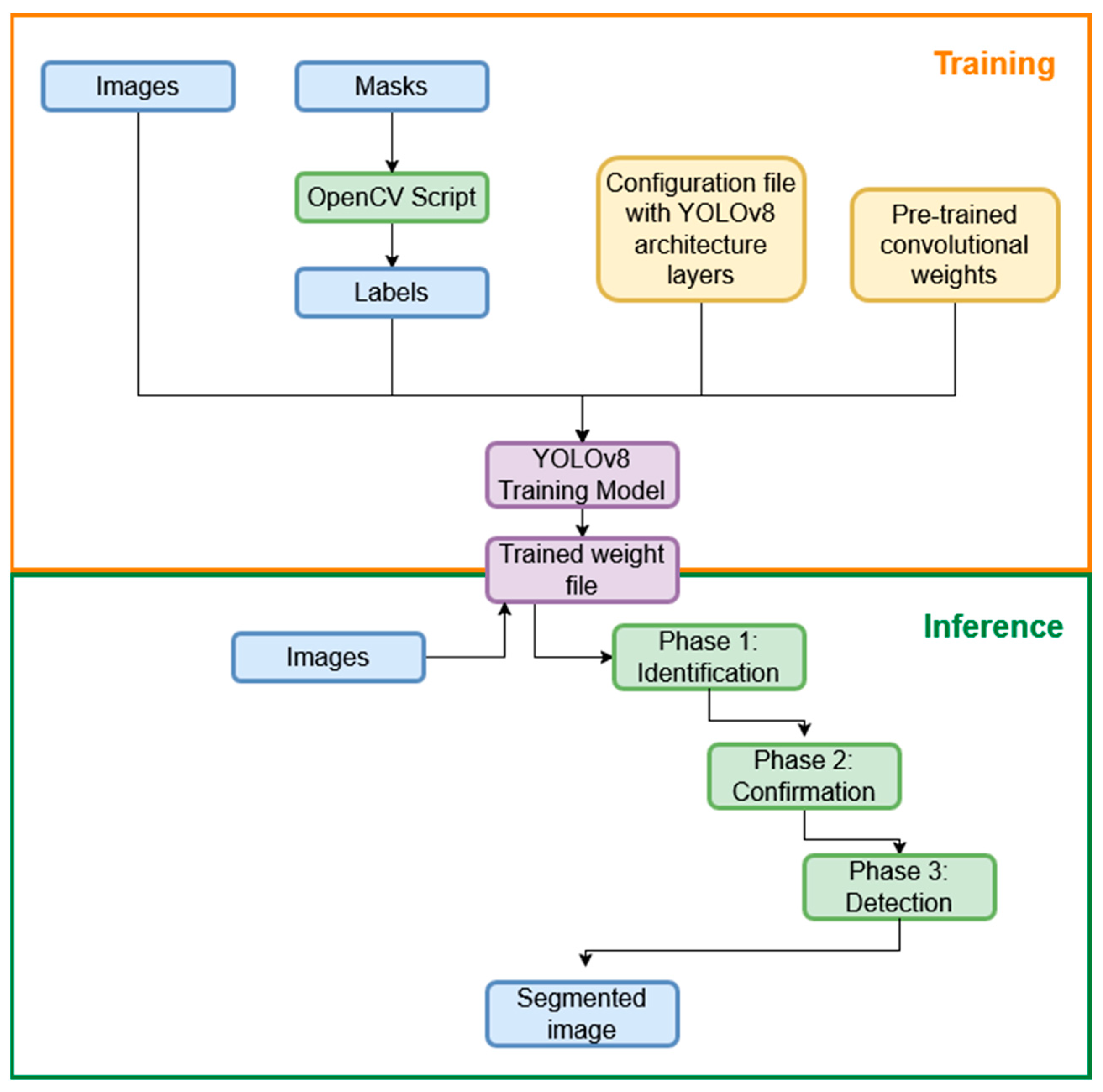
The object recognition model creation and validation include four tasks: image dataset creation, labelling of these images, training of the object recognition model and its validation.
Creating the image dataset includes using the Common Object in Context (COCO) [120] dataset, an open-source computer vision dataset for common elements (e.g., people, bicycles, cars, motorcycles, buses, traffic lights, laptops, among others). However, for more specific objects for this type of scene (e.g., traffic cones, skid marks, guns, knives, cartridges, bullet holes, blood stains, among others), it was necessary to collect the categories of objects manually to create a dataset that contained instances of the key evidence objects.
For image labelling, the OpenCV library was used to program a script to automate the task. The script takes the masks as input and from them identifies the silhouette of the object. As a result, a YOLOv8-compatible text file is generated in which the object class is detailed along with the polygon that delimits its contour. Finally, the model training task was carried out using the images and labels and then proceeded to validate the model.
It can be seen that in this process there are two differentiated stages: training and inference, as detailed in Figure 8.
Ballistic analysis
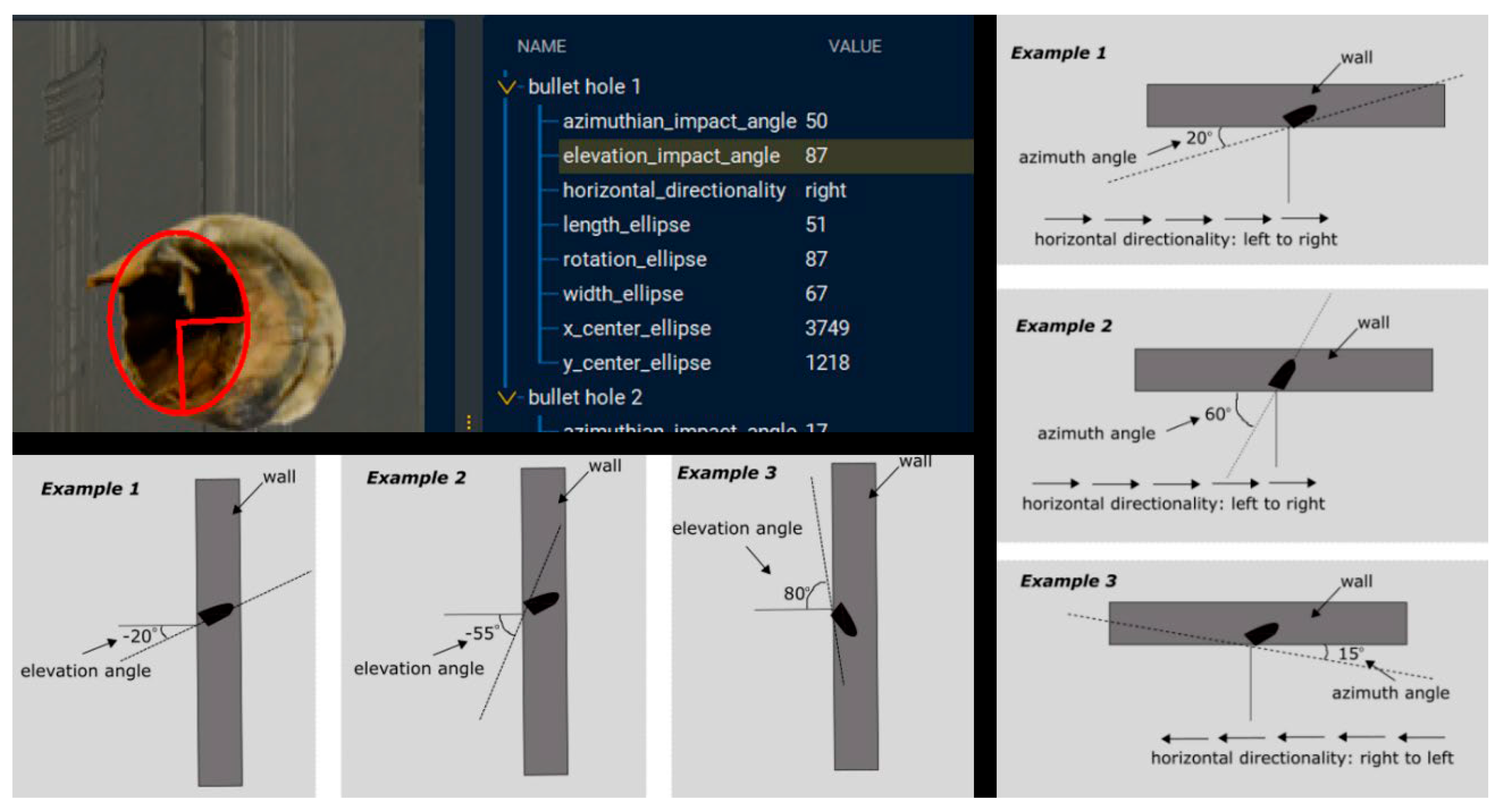
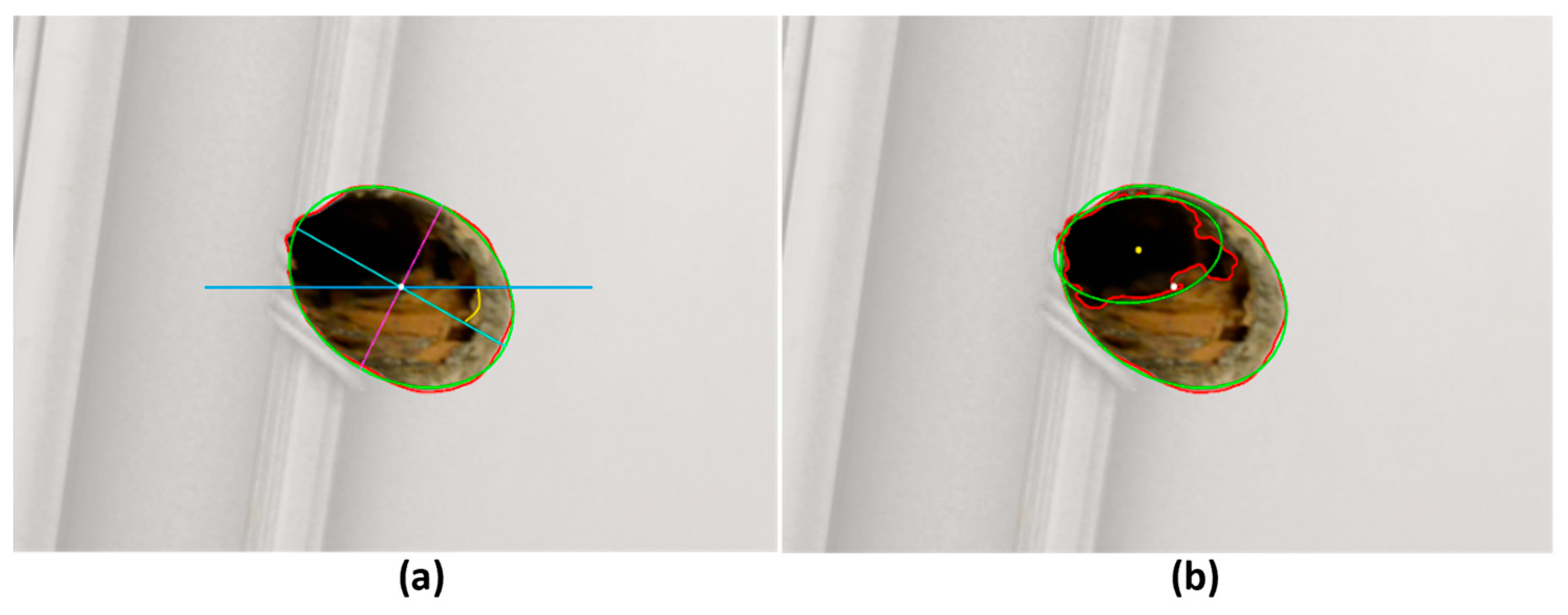
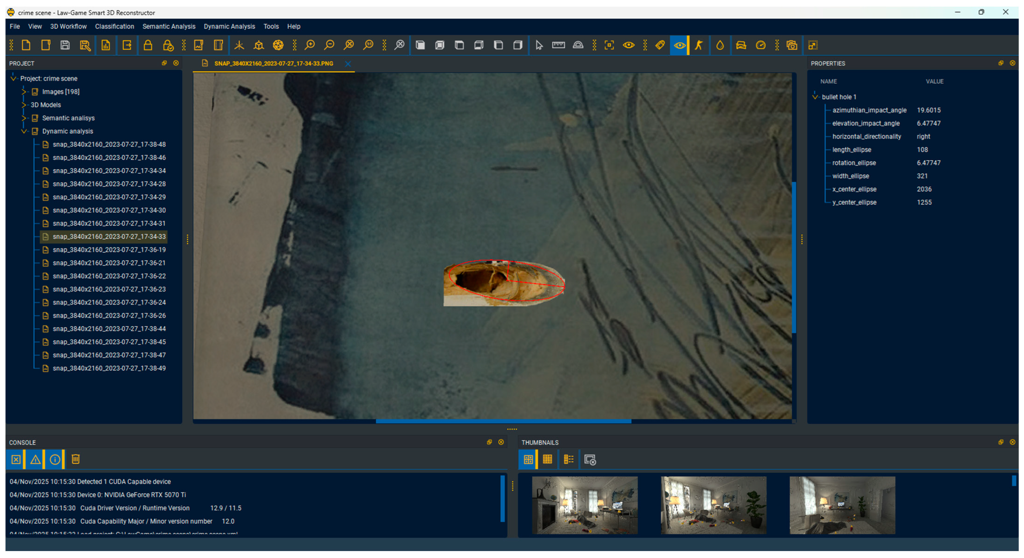
The tool detects bullet impacts in the acquired images and generates a JSON file containing essential information. This file includes the central location of each bullet hole, as well as a calculated directional vector defined by the elevation angle (ranging from −90 to +90 degrees) and the azimuth angle (0 to 90 degrees) at which a bullet penetrated the impact surface as well as the horizontal directionality of the bullet (i.e., right to left or vice versa) (Figure 9). These details are derived from images captured at optimal angles to ensure they are as orthogonal as possible to the surface of the bullet holes and as close as feasible for accurate measurement. Specifically, after optimal images of bullet impacts are acquired, they undergo a series of advanced artificial intelligence, computer vision and image processing techniques [121]. The purpose of this analysis is to ultimately define a number of ellipses (one ellipse per bullet impact (Figure 10a, green outline)), from the computed contours (Figure 10a, red outline) of the bullet holes, capturing the whole impact surface of the bullet hole. Some features are obtained from each aforementioned ellipse: (a) its length (minor axis (Figure 10a, purple line)), (b) its width (major axis (Figure 10a, cyan line)) and (c) its rotation (according to the Cartesian coordinate system established to the centre of the ellipse (Figure 10a, yellow curve)). From these, the azimuth and elevation angles are calculated by applying the following equations.
a = s i n 1 l w
e = r
  • a: azimuth angle
  • l: ellipse length (minor axis)
  • w: ellipse width (major axis)
  • e: elevation angle
  • r: ellipse rotation
Figure 9. Bullet hole analysis module and associated explanations on how elevation and azimuth angles are calculated in various scenarios.
Algorithms 18 00707 g009
Figure 10. Bullet hole image analysis.
Algorithms 18 00707 g010
The horizontal directionality of the bullet can be estimated through a similar analysis of only the darkest area of the bullet hole (compared to the whole impact surface), presumed to be the point of deepest penetration (Figure 10b).
Using the JSON data as a basis, the tool computes potential projectile trajectories1 and identifies intersecting points. This analysis is intended to infer the shooter’s position.
If multiple bullet holes are present and identified at the crime scene, the final step involves checking for possible intersections among each pair of the computed trajectories. When at least two bullet trajectories intersect, the intersection point is considered a probable location of the shooter or perpetrator at the time of the shooting. In cases where multiple intersection points are identified, it may also indicate the shooter’s movement within the crime scene.
Impact speed estimation for car accidents
The Equivalent Barrier Speed (EBS) is a crucial metric in accident reconstruction, calculated by equating the vehicle’s kinetic energy with the energy absorbed during plastic deformation. This method, frequently used in forensic investigations, involves advanced 3D analysis utilizing specialized tools and methodologies.
Forensic analysts employ the Prasad Method to compute energy absorption during collisions with rigid barriers. This approach quantifies the absorbed energy by integrating various deformation measures into the following formula (Equation (4)):
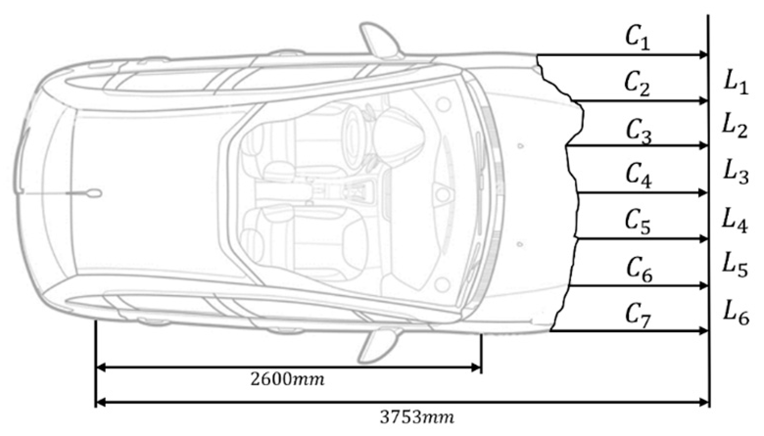
E d = L d 0 2 2 + i = 1 , n L c d 0 d 1 c i c i 1 2 + c i 1 + d 1 2 2 c i c i 1 2 3 + c i 1 2 + c i c i 1 c i 1
  • L: Width of the deformed area.
  • d0, d1: Prasad coefficients
  • ci: Deformation measurements
  • Lc: Distances between measurements
The Prasad coefficients (d0, d1), which are specific to each vehicle type and collision category, are detailed in the table below (Table 3):
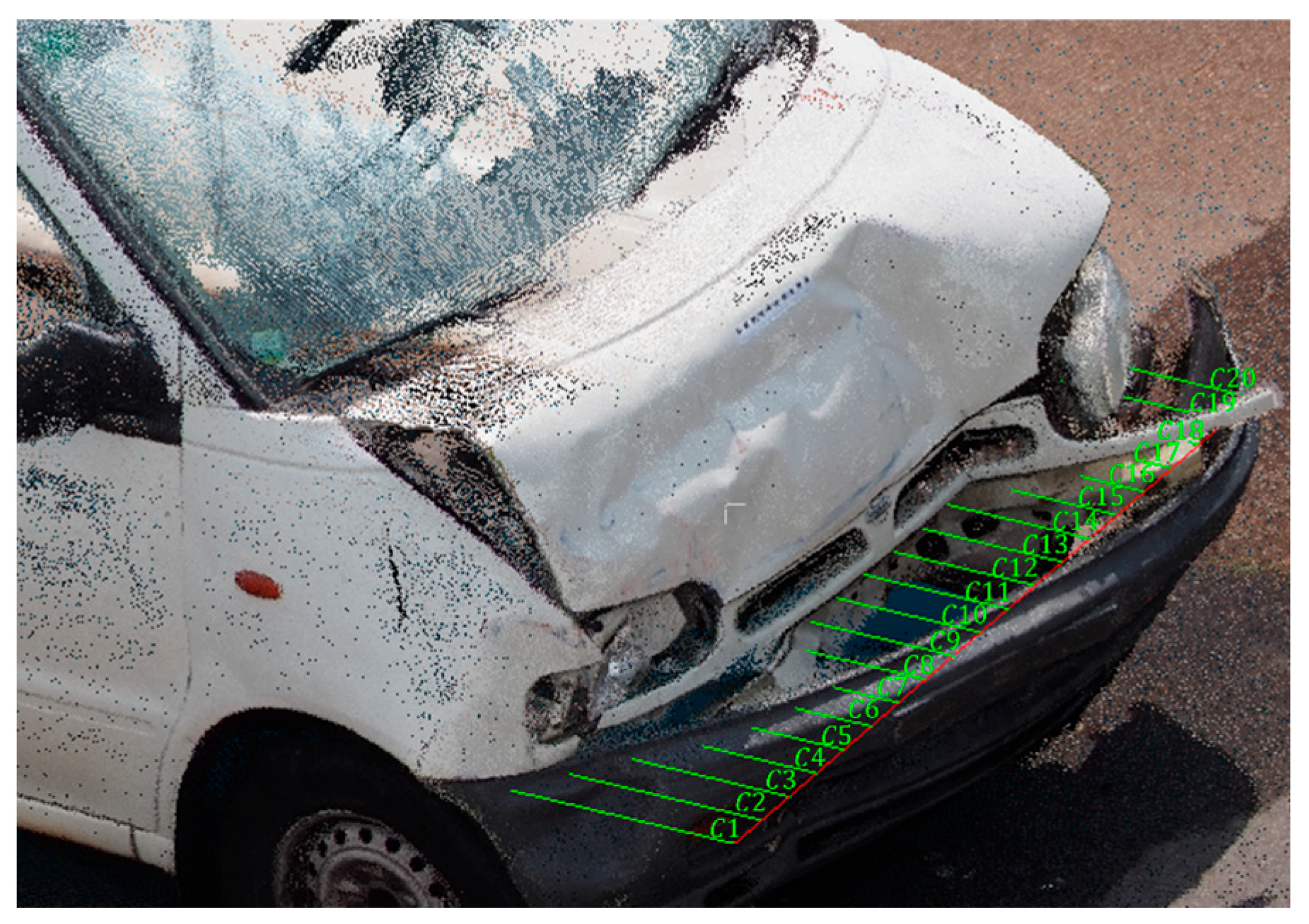
Deformation measurement involves segmenting the length of the deformed area and assessing the depth of the deformation relative to a reference measure (Figure 11).
From the energy of deformation (Equation (5)), the Equivalent Barrier Speed (EBS) is determined using the formula:
E B S = 2 E d m
  • m : mass of the vehicle.
  • E d : energy absorbed during the collision
In forensic investigations, this comprehensive calculation methodology (integrating advanced 3D analysis and precise deformation measurements) enables an accurate determination of the Equivalent Barrier Speed (EBS). This metric is critical for understanding the dynamics of a collision and assessing the severity of the impact, aiding forensic analysts in reconstructing the events leading to a crash with greater precision and reliability.

3. Results

To verify the tool’s functionality, tests were conducted on two scenarios: a simulated real traffic accident and a simulated crime scene created using Unity3D 2021.3.4f1.

3.1. Car Accident Scenario

This section presents the results of the tests conducted on the traffic accident scene.

3.1.1. Three-Dimensional Reconstruction

  • The first step involves uploading the traffic accident photos into the tool (Figure 12). For this scenario, the convergent protocol was applied to capture images to reconstruct the entire scene. A total of 61 photographs were taken in this case.
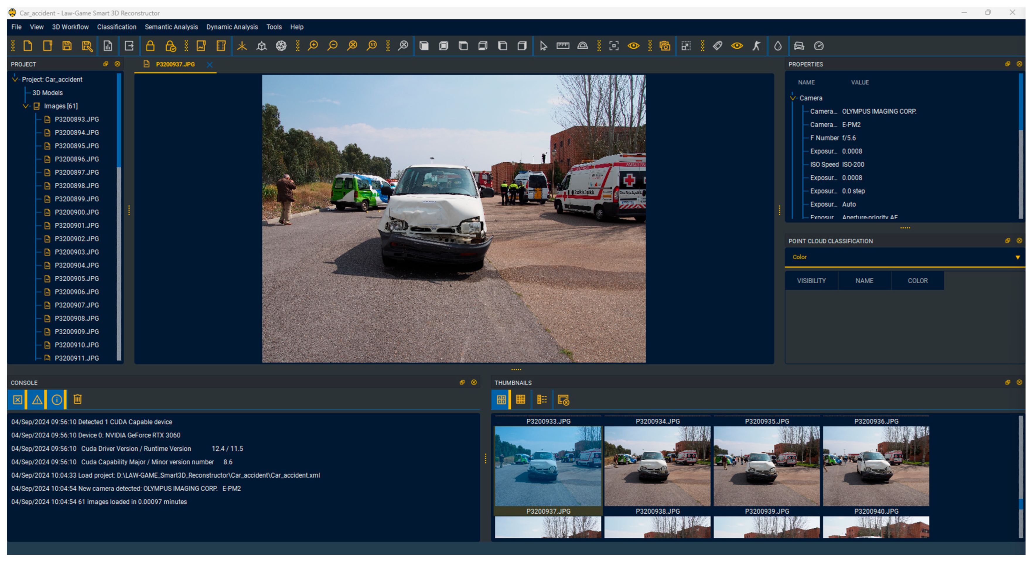
Figure 12. Uploading photos of the car accident.
Algorithms 18 00707 g012
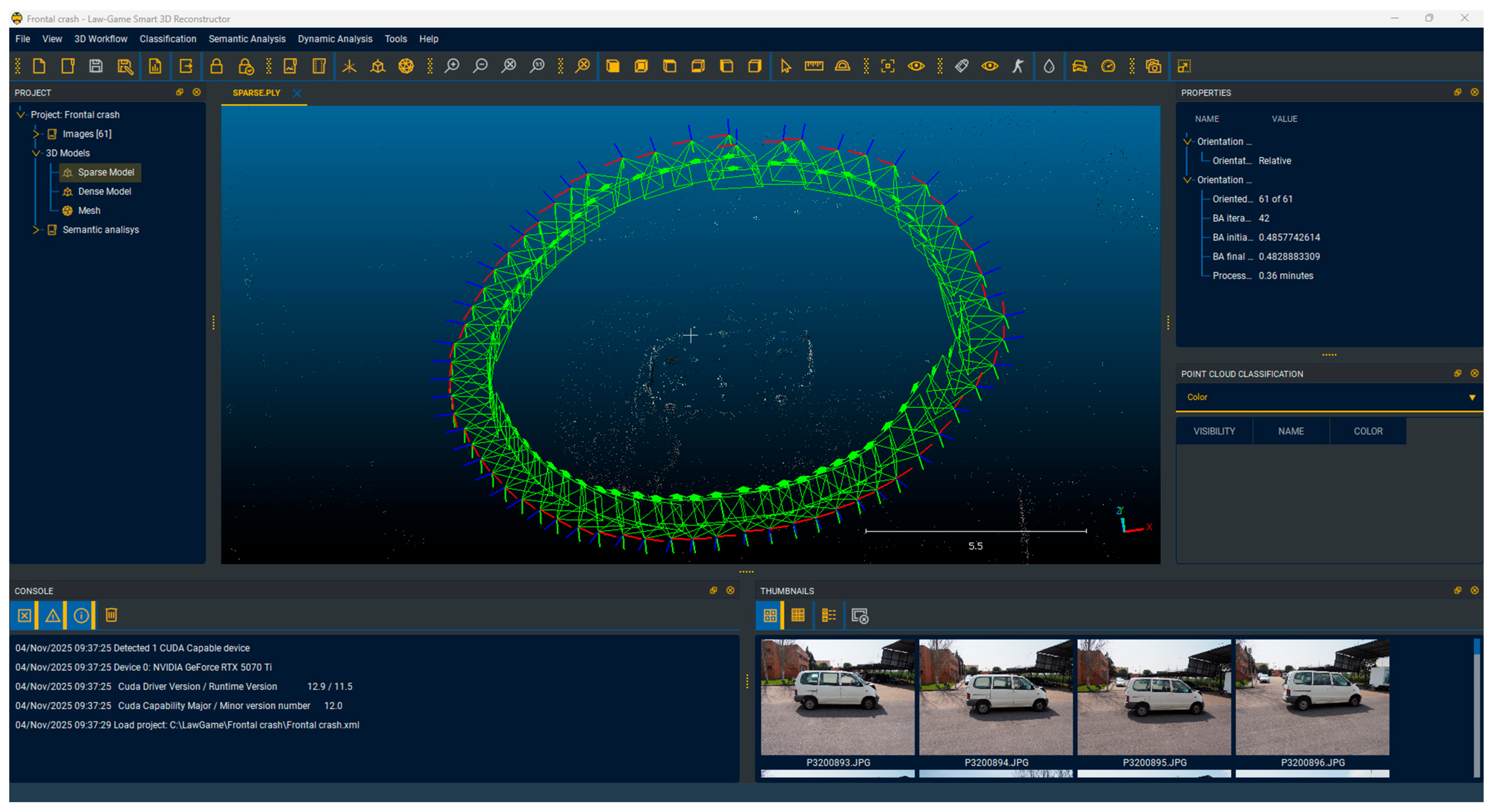
Once the photos have been uploaded, the 3D reconstruction of the scene can begin. First the feature extraction was performed using the SIFT algorithm; in the case 278,077 features were detected. Also, the matching strategy was executed obtaining 121,888 matches. The next step is to generate the sparse model (Figure 13), which establishes the different camera orientations during the image acquisition process; in this case, all 61 photographs were successfully orientated. This process includes the camera self-calibration and thus the estimation of the internal camera parameters, that for this case are shown in Table 4.
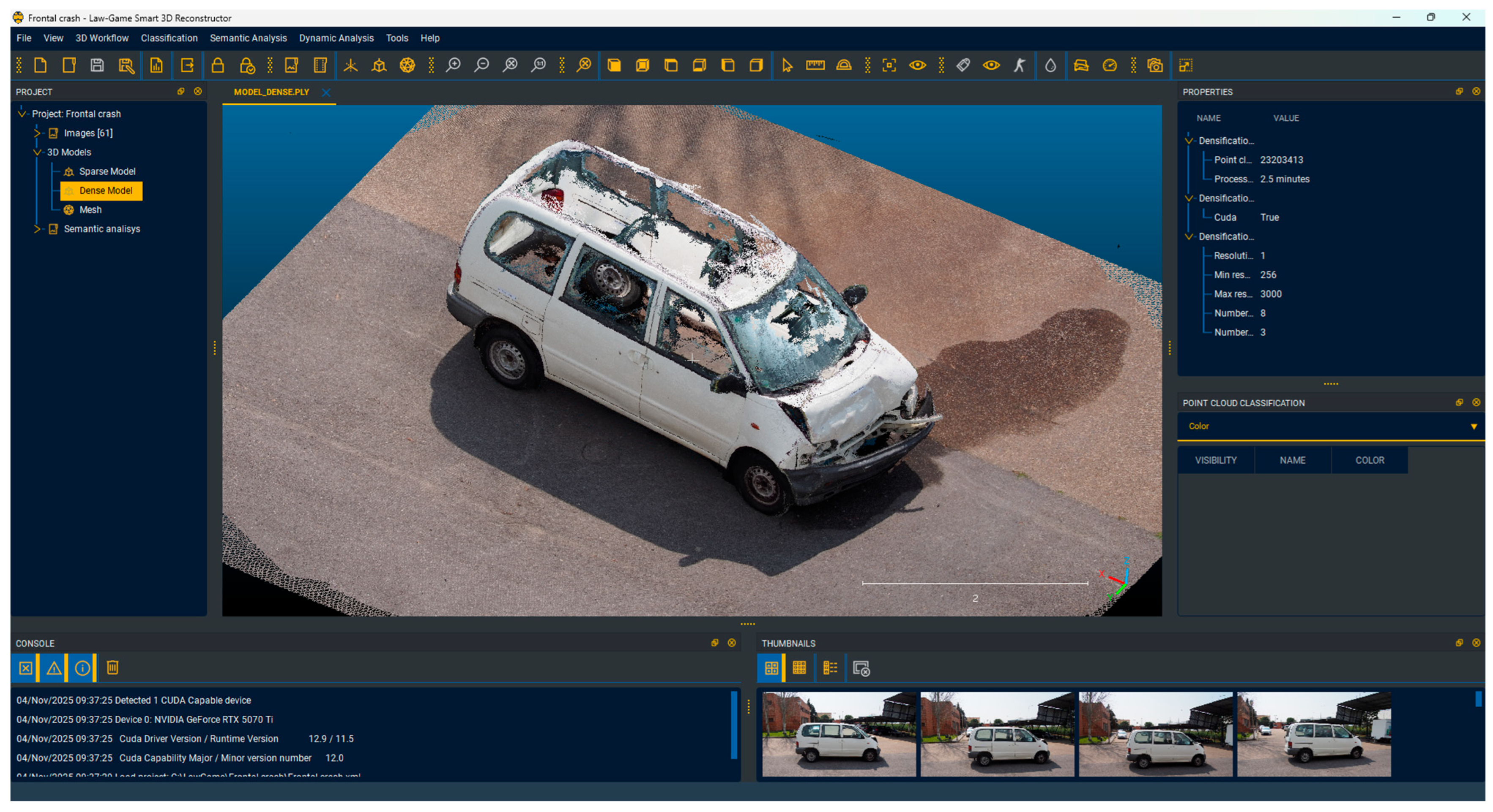
Subsequently, it is possible to generate the 3D point cloud of the scene (Figure 14) applying the MVS algorithm. This 3D model was generated with a total of 23,203,413 points.
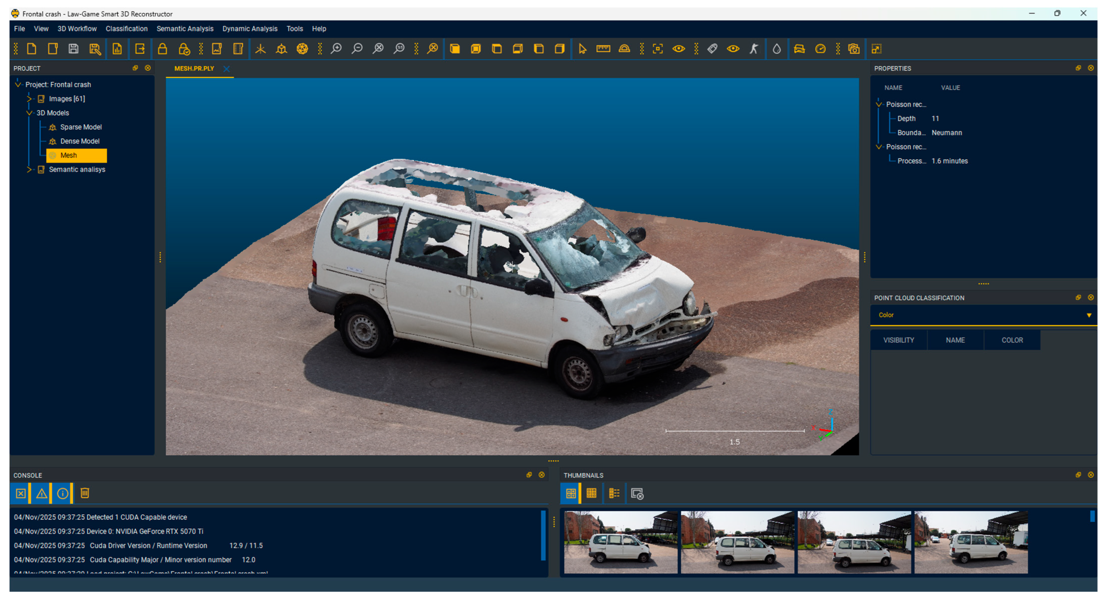
Finally, a mesh can be obtained (Figure 15) applying a generation strategy based on Poisson Surface Reconstruction, providing a more complete 3D model of the scene.

3.1.2. Semantic Analysis

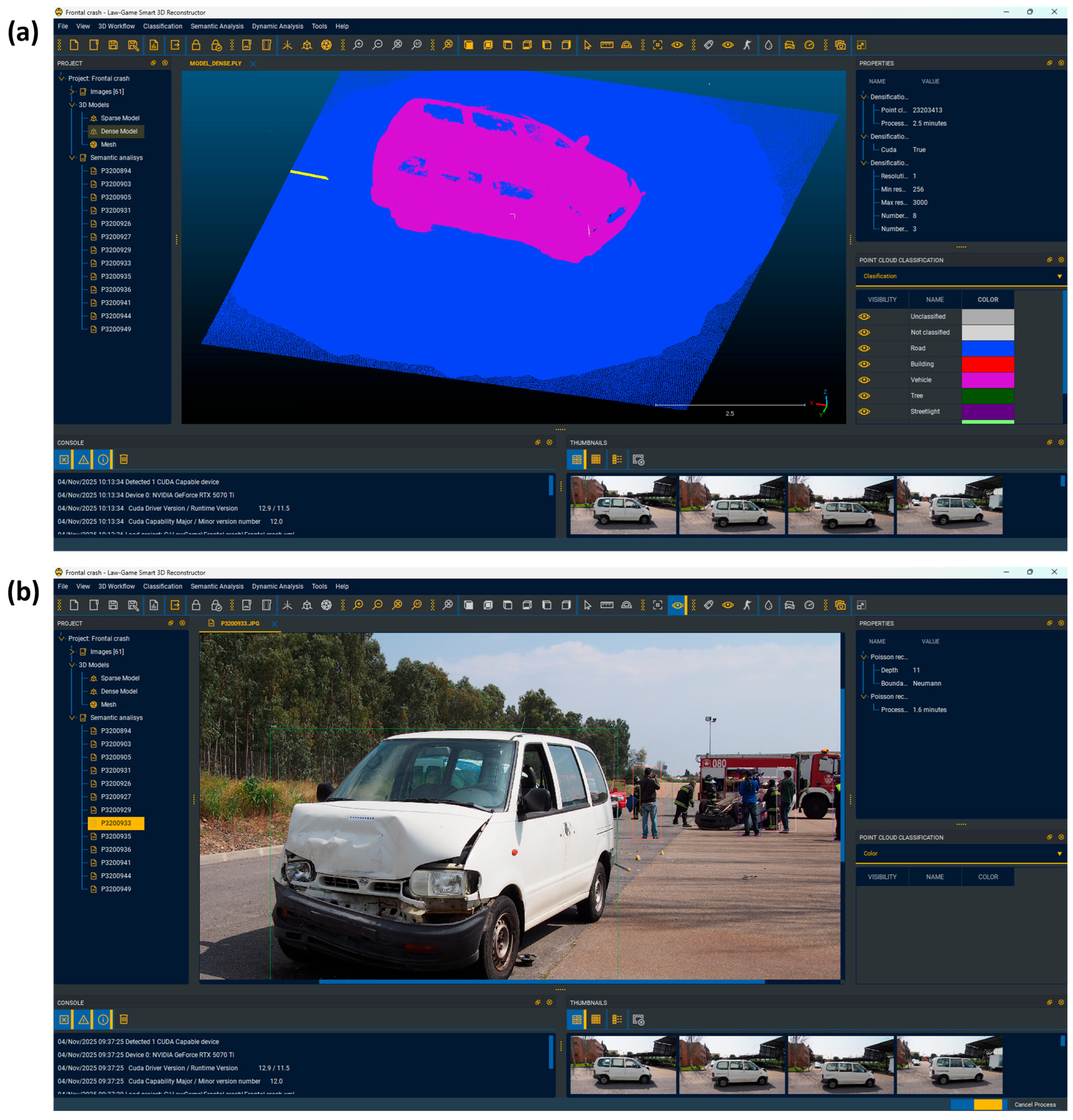
Once the 3D models are obtained, a semantic analysis can be performed, which includes point cloud classification and object detection in images (Figure 16).

3.1.3. Dynamic Analysis

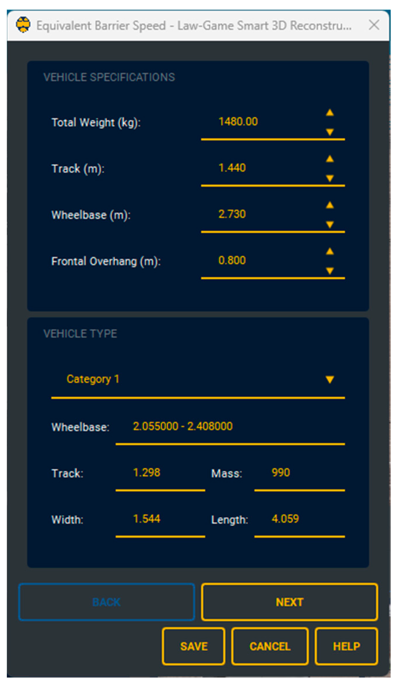
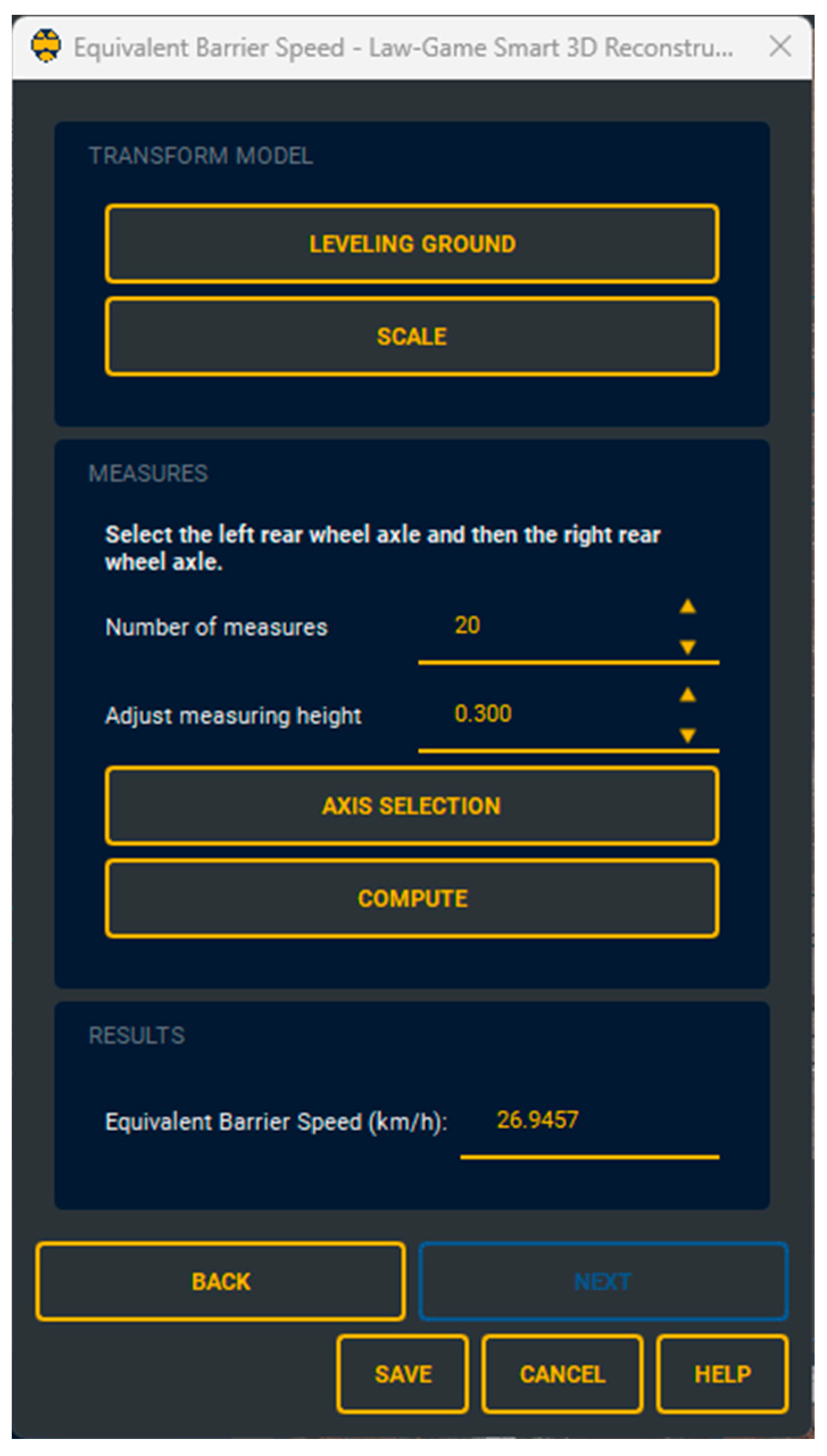
Finally, dynamic analysis can be conducted to estimate the car’s impact speed. This analysis requires the user to complete a form with information about the vehicle in question (Figure 17) and then select the centers of the rear wheel axles to calculate the deformation measurements (Figure 18 and Table 5).
Finally, the impact speed was calculated using the Equivalent Barrier Speed formula (Equation (5)) and shown in the tool (Figure 19). In this case, the deformation energy was 41,457.8 Jules and the equivalent barrier speed 26.95 km/h.

3.2. Crime Scene

This section, in turn, presents the results obtained from the analysis of the simulated crime scene.

3.2.1. Three-Dimensional Reconstruction

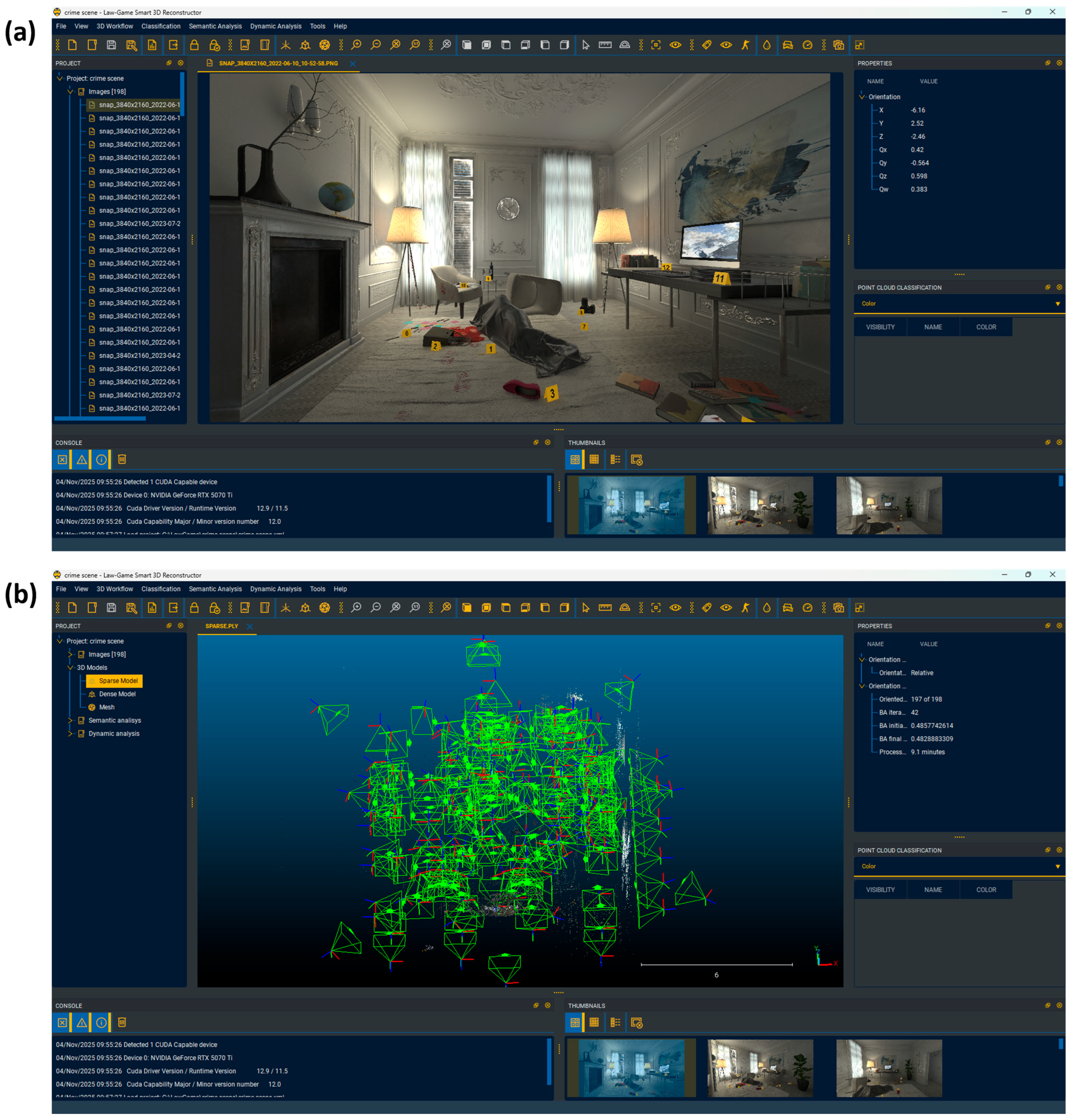
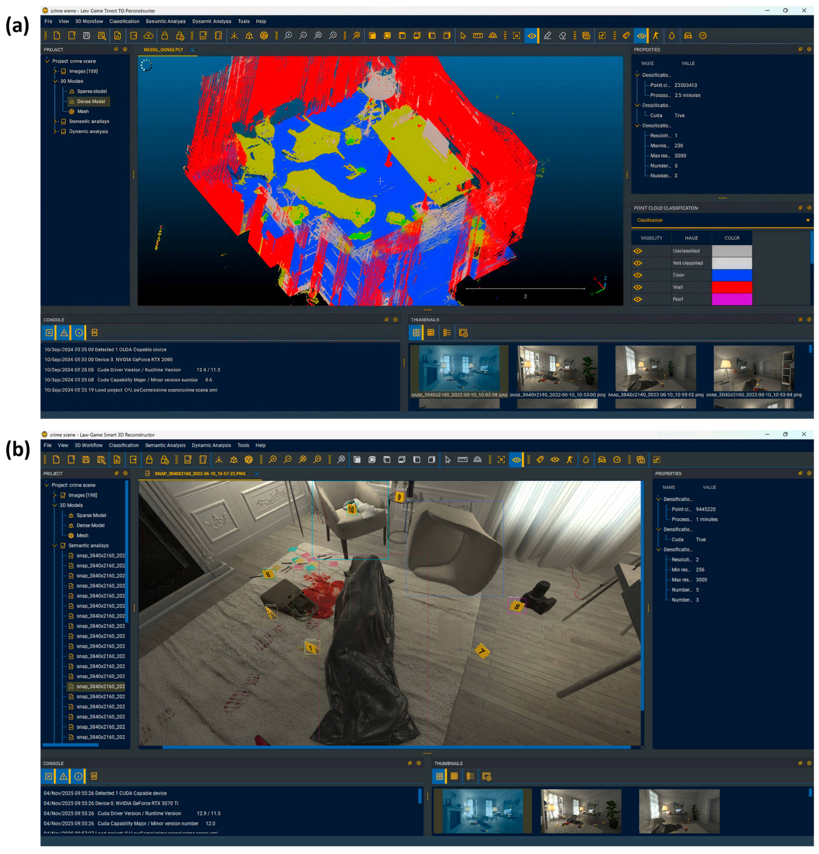
The photos were acquired using the convergent protocol to obtain a complete 3D model of scene, but also the parallel protocol was applied to obtain detailed pictures of key evidence (e.g., bullet holes). A total of 198 images were used to reconstruct this simulated crime scene.
As in the previous case, the first step involves uploading the images (Figure 20a), in this case through the feature extraction task 291,283 were detected and applying the matching strategy 565,433 matches were encountered. The next step is generating the sparse model of the scene (Figure 20b); the orientation process allowed to solve the spatial and angular position of 141 images out of the 198 uploaded. Images that do not comply with the acquisition protocols described in Section 2, particularly those violating basic photogrammetry principles, are automatically discarded by the software to prevent reconstruction errors. The camera self-calibration and the estimation of the internal camera parameters are shown in Table 6.
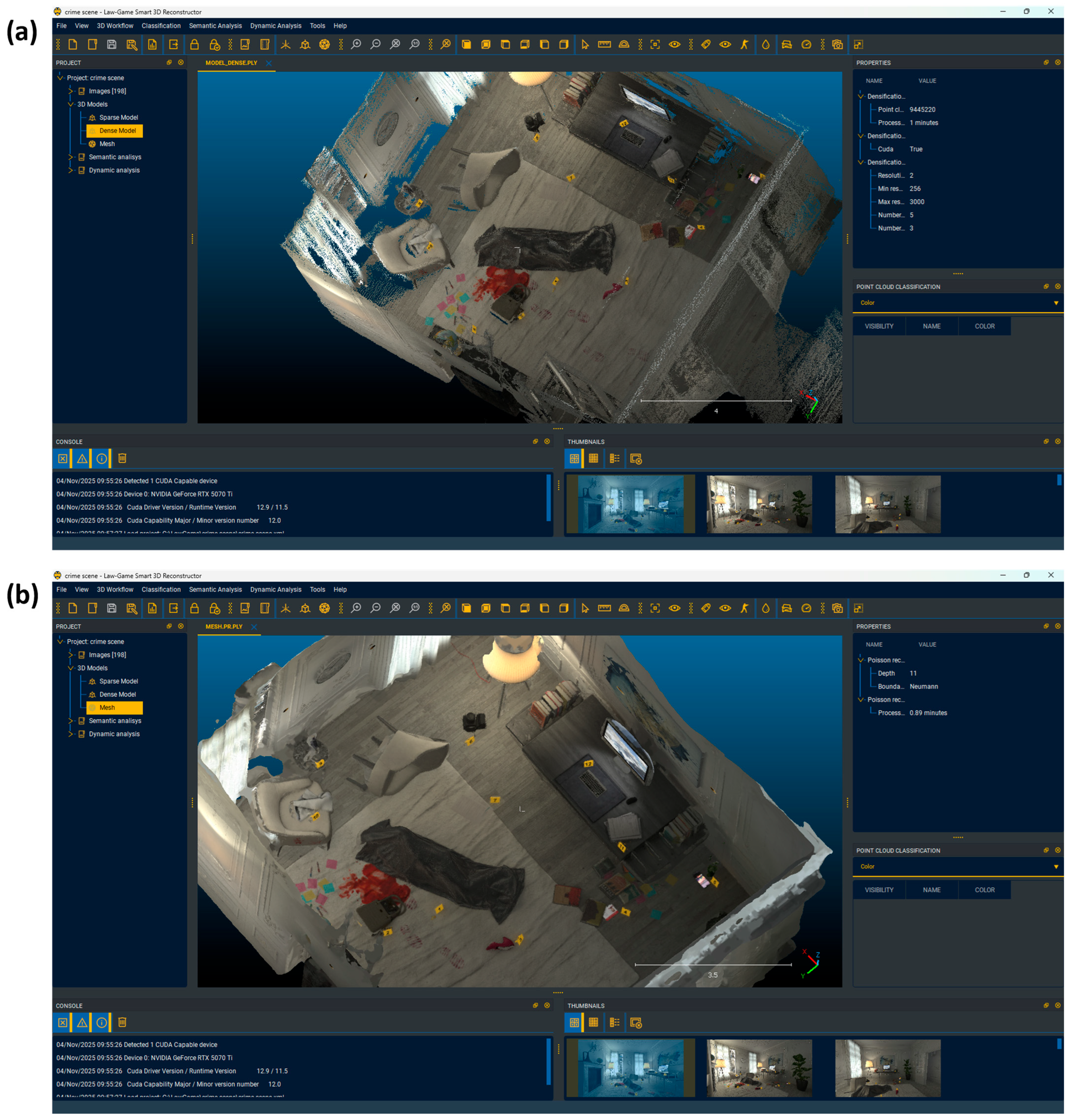
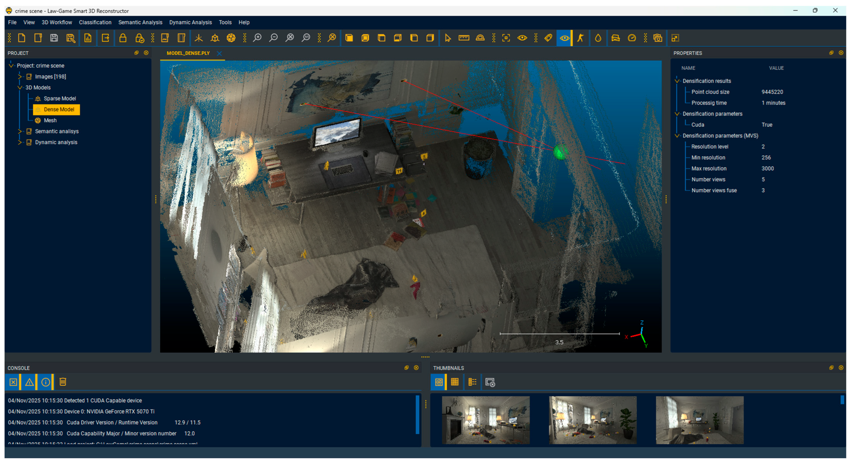
Once the sparse model has been obtained, the dense model (Figure 21a) and the mesh (Figure 21b) of the scene are generated. In this case, the resulting dense model has 23,203,413 points.

3.2.2. Semantic Analysis

After obtaining the 3D models, a semantic analysis was conducted on both the point cloud and the images (Figure 22).

3.2.3. Dynamic Analysis

First, through semantic analysis, the images where bullet holes have been detected are identified, and in these images, the various characteristics of the detected holes are determined (azimuthian and elevation impact angle, horizontal directionality, ellipse length and width, among others). In this case, two bullet holes were detected and the characteristics extracted are shown in Table 7 and Figure 23.
The bullet holes’ positions and trajectories vectors were calculated from the features extracted and the results are shown in Table 8.
Finally, as in this case, the bullet trajectories intersect, and thus the shooter’s position can be estimated based on this intersection (Figure 24). The coordinates of the estimated shooter position are (−2.286, −0.437, −0.690).

4. Discussion

This article first presents various methods and software tools for 3D forensic digitization and reconstruction. It then introduces an innovative tool that integrates multiple modules, covering various tasks that security agencies must perform to conduct forensic investigations in crime scenes and traffic accidents.
This comprehensive tool integrates essential modules to ensure accurate investigations in this field, including 3D scene reconstruction for long-term preservation, semantic analysis for detecting investigation-relevant objects, and dynamic analysis for studying ballistic trajectories and estimating vehicle impact speed in traffic accidents.
The 3D reconstruction module allows the recreation of a scene from images or videos captured according to the acquisition protocols outlined in Section 2.2.1 of this study. The output includes various 3D models: a sparse model (indicating the camera positions during image acquisition), a dense model (3D point cloud of the scene), and a mesh (a more complete 3D model). Section 3 demonstrates the tool’s ability to achieve accurate results, highlighting the capabilities of photogrammetry in this field.
Once the scene has been reconstructed in 3D, the tool enables dynamic analysis, identifying objects relevant to forensic scene investigations. This analysis includes the classification of the 3D point cloud using the random forest model, as well as object detection in images through YOLOv8. These two tasks are interconnected, as the detected objects in the images can be localized within the point cloud by applying photogrammetric principles.
Finally, the tool includes a dynamic analysis module that enables ballistic trajectory analysis in crime scenes and impact speed analysis for traffic accident scenarios. The ballistic analysis is based on the detection of bullet holes and the extraction of key data, such as the location of the hole’s center and the directional vector specifying the elevation angle. On the other hand, the impact speed analysis is based on the calculation of the Equivalent Barrier Speed (EBS), derived from the deformation of the vehicles involved in the traffic accident.
Embedding all these modules within a single tool, along with its user-friendly and accessible interface for non-experts, represents the main advantage and improvement over existing tools. Most current tools focus on a single task (reconstruction, semantic analysis, or dynamic analysis) and are typically not user-friendly, which presents a significant drawback. Therefore, the tool presented in this article offers a comprehensive solution with a high capacity to support end users in forensic investigations, even if they are not experts in photogrammetry or machine learning.

Author Contributions

Conceptualization, A.O.-B., E.R.d.O. and D.G.-A.; methodology, A.O.-B., E.R.d.O. and R.Y.; software, A.O.-B., E.R.d.O. and E.P.; validation, A.O.-B., R.Y. and K.M.; investigation, A.O.-B. and E.P.; resources, A.O.-B. and D.G.-A.; writing—original draft preparation, A.O.-B. and E.P.; writing—review and editing, A.O.-B., E.R.d.O., R.Y., E.P., K.M. and D.G.-A.; supervision, A.O.-B.; project administration, A.O.-B. and D.G.-A.; funding acquisition, D.G.-A. All authors have read and agreed to the published version of the manuscript.

Funding

This research received no external funding.

Data Availability Statement

The datasets presented in this article are not readily available because they are part of the European Project H2020 LAW-GAME, and the data provided by end-users—primarily police forces from various European countries—are confidential. Requests to access the datasets should be directed to the corresponding author.

Acknowledgments

This research was supported by the European Project H2020 LAW-GAME: An Interactive, Collaborative Digital Gamification Approach to Effective Experiential Training and Prediction of Criminal Actions. Authors would also like to thank the TIDOP Research Group of the Department of Cartographic and Land Engineering of the Higher Polytechnic School of Ávila (University of Salamanca).

Conflicts of Interest

The authors declare no conflicts of interest.

Abbreviations

The following abbreviations are used in this manuscript:
EBSEquivalent Barrier Speed
ABSAnti-lock braking system
SfMStructure from Motion
UAVUnmanned aerial vehicle
DEMDigital elevation model
GUIGraphical user interface
ODMOpen Drone Map
GCPGround control point
MVEMulti-view environment
ABMArea-based matching
LSMLeast Squares Matching
SUSANSmallest Univalue Segment Assimilation Nucleus
MSEREfficient Maximally Stable Extremal Region
SURFSpeeded Up Robust Features
SIFTScale Invariant Feature Transform
RANSACRandom Sample Consensus
DLTDirect Linear Transformation
SGMSemi-Global Matching
COCOCommon Object in Context

References

  1. Stuart, H.J.; Nordby, J.J.; Bell, S. Forensic Science: An Introduction to Scientific and Investigative Techniques; CRC Press: Boca Raton, FL, USA, 2002. [Google Scholar]
  2. Docchio, F.; Sansoni, G.; Tironi, M.; Bui, C. Sviluppo di procedure di misura per il rilievo ottico tridimensionale di scene del crimine. In Proceedings of the XXIII Congresso Nazionale Associazione Gruppo di Misure Elettriche ed Elettroniche, L’Aquila, Italy, 11–13 September 2006. [Google Scholar]
  3. Kovacs, L.; Zimmermann, A.; Brockmann, G.; Gühring, M.; Baurecht, H.; Papadopulos, N.A.; Zeilhofer, H.F. Three-dimensional recording of the human face with a 3D laser scanner. J. Plast. Reconstr. Aesthetic Surg. 2006, 59, 1193–1202. [Google Scholar] [CrossRef]
  4. Cavagnini, G.; Sansoni, G.; Trebeschi, M. Using 3D range cameras for crime scene documentation and legal medicine. In Proceedings of the the SPIE—The International Society for Optical Engineering, San Diego, CA, USA, 2–6 August 2009. [Google Scholar]
  5. Sansoni, G.; Trebeschi, M.; Docchio, F. State-of-The-Art and Applications of 3D Imaging Sensors in Industry, Cultural Heritage, Medicine, and Criminal Investigation. Sensors 2009, 9, 568–601. [Google Scholar] [CrossRef] [PubMed]
  6. Pastra, K.; Saggion, H.; Wilks, Y. Extracting relational facts for indexing and retrieval of crime-scene photographs. Knowl.-Based Syst. 2003, 16, 313–320. [Google Scholar] [CrossRef]
  7. Gonzalez-Aguilera, D.; Gomez-Lahoz, J. Forensic terrestrial photogrammetry from a single image. Forensic Sci. 2009, 54, 1376–1387. [Google Scholar] [CrossRef]
  8. D’Apuzzo, N.; Harvey, M. Medical applications. In Advances in Photogrammetry, Remote Sensing and Spatial Information Sciences: 2008 ISPRS Congress Book; CRC Press: Boca Raton, FL, USA, 2008; pp. 443–456. [Google Scholar]
  9. Rönnholm, P.; Honkavaara, E.; Litkey, P.; Hyyppä, H.; Hyyppä, J. Integration of Laser Scanning and Photogrammetry. Int. Arch. Photogramm. Remote Sens. Spat. Inf. Sci 2006, 36, 355–362. [Google Scholar]
  10. El-Hakim, S.; Beraldin, J.-A.; Blais, F. A Comparative Evaluation of the Performance of Passive and Active 3-D Vision Systems. In Proceedings of the SPIE—The International Society for Optical Engineering, San Diego, CA, USA, 4–8 August 2003. [Google Scholar]
  11. Remondino, F.; Guarnieri, A.; Vettore, A. 3D modeling of Close-Range Objects: Photogrammetry or Laser Scanning. In Proceedings of the SPIE, Kissimmee, FL, USA, 12–16 April 2004. [Google Scholar]
  12. Remondino, F.; Fraser, C. Digital camera calibration methods: Considerations and comparisons. Ine. Arch. Photogramm. Remote Sens. Spat. Inf. Sci. 2005, 36, 266–272. [Google Scholar]
  13. Apero-Micmac Open Source Tools. Available online: http://www.tapenade.gamsau.archi.fr/TAPEnADe/Tools.html (accessed on 5 August 2024).
  14. Cloud Compare Open Source Tool. Available online: http://www.danielgm.net/cc/ (accessed on 5 August 2024).
  15. Deseilligny, M.; Clery, I. APERO, an open source bundle adjusment software for automatic calibration and orientation of set of images. ISPRS Int. Arch. Photogramm. Remote Sens. Spat. Inf. Sci. 2011, XXXVIII-5/W16, 269–276. [Google Scholar] [CrossRef]
  16. Samaan, M.; Heno, R.; Deseilligny, M. Close-range photogrammetric tools for small 3D archeological objects. ISPRS Int. Arch. Photogramm. Remote Sens. Spat. Inf. Sci. 2013, XL-5/W2, 549–553. [Google Scholar] [CrossRef]
  17. Mildenhall, B.; Srinivasan, P.P.; Tancik, M.; Barron, J.T.; Ramamoorthi, R.; Ng, R. NeRF: Representing Scenes as Neural Radiance Fields for View Synthesis. Commun. ACM 2021, 65, 99–106. [Google Scholar] [CrossRef]
  18. Ponto, K.; Tredinnick, R. Opportunities for utilizing consumer grade 3D capture tools for insurance documentation. Int. J. Inf. Technol. 2022, 14, 2757–2766. [Google Scholar] [CrossRef]
  19. Martin-Brualla, R.; Radwan, N.; Sajjadi, M.S.M.; Barron, J.T.; Dosovitskiy, A.; Duckworth, D. NeRF in the Wild: Neural Radiance Fields for Unconstrained Photo Collections. In Proceedings of the Computer Vision and Pattern Recognition, Nashville, TN, USA, 20–25 June 2021. [Google Scholar]
  20. Pumarola, A.; Corona, E.; Pons-Moll, G.; Moreno-Noguer, F. D-NeRF: Neural Radiance Fields for Dynamic Scenes. In Proceedings of the Computer Vision and Pattern Recognition, Nashville, TN, USA, 20–25 June 2021. [Google Scholar]
  21. Tretschk, E.; Tewari, A.; Golyanik, V.; Zollhöfer, M.; Lassner, C.; Theobalt, C. Non-Rigid Neural Radiance Fields: Reconstruction and Novel View Synthesis of a Dynamic Scene From Monocular Video. In Proceedings of the Computer Vision and Pattern Recognition, Nashville, TN, USA, 20–25 June 2021. [Google Scholar]
  22. Wang, Z.; Wu, S.; Xie, W.; Chen, M.; Prisacariu, V.A. NeRF--: Neural Radiance Fields Without Known Camera Parameters. In Proceedings of the Computer Vision and Pattern Recognition, Nashville, TN, USA, 20–25 June 2021. [Google Scholar]
  23. Zhu, H.; Wu, W.; Zhu, W.; Jiang, L.; Tang, S.; Zhang, L.; Liu, Z.; Loy, C.C. CelebV-HQ: A Large-Scale Video Facial Attributes Dataset. In Proceedings of the European Conference on Computer Vision, Tel Aviv, Israel, 23–27 October 2022. [Google Scholar]
  24. Rodríguez, M.U.P.; Álvarez, J.A.S.; Cárdenas, J.G.M. Investigación & Reconstrucción de accidentes: La Reconstrucción práctica de un accidente de tráfico. Secur. Vialis 2011, 1, 27–37. [Google Scholar] [CrossRef]
  25. Sánchez, J.L.D.; Andreu, J.S.-F. La reconstrucción de accidentes desde el punto de vista policial. Cuad. Guard. Civ. Rev. Segur. Pública 2004, 1, 109–118. [Google Scholar]
  26. Carballo, H. Pericias Tecnico-Mecanicas; Ediciones Larocca: Buenos Aires, Argentina, 2005. [Google Scholar]
  27. Robsan, S.; Kyle, S.; Harley, I. Close Range Photogrammetry: Principles, Techniques and Applications; Whittles Publishing: Hertfordshire, UK, 2011. [Google Scholar]
  28. González-Aguilera, D.; Muñoz-Nieto, Á.; Rodríguez-Gonzalvez, P.; Mancera-Taboada, J. Accuracy assessment of vehicles surface area measurement by means of statistical methods. Measurement 2013, 46, 1009–1018. [Google Scholar] [CrossRef]
  29. Du, X.; Jin, X.; Zhang, X.; Shen, J.; Hou, X. Geometry features measurement of traffic accident for reconstruction based on close-range photogrammetry. Adv. Eng. Softw. 2009, 40, 497–505. [Google Scholar] [CrossRef]
  30. Fraser, C.; Hanley, H.; Cronk, S. Close-range photogrammetry for accident reconstruction. In Optical 3D Measurements VII; Gruen, A., Kahmen, H., Eds.; SPIE: Bellingham, WA, USA, 2005; Volume 2, pp. 115–123. [Google Scholar]
  31. Fraser, C.; Cronk, S.; Hanley, H. Close-range photogrammetry in traffic incident management. In Proceedings of the XXI ISPRS Congress Commission V, Beijing, China, 3–11 July 2008. [Google Scholar]
  32. Hattori, S.; Aklmoto, K.; Fraser, C.; Imoto, H. Automated procedures with coded targets in industrial vision metrology. Photogramm. Eng. Remote Sens. 2002, 68, 441–446. [Google Scholar]
  33. Han, I.; Kang, H. Determination of the collision speed of a vehicle from evaluation of the crush volume using photographs. Proc. Inst. Mech. Eng. Part D J. Automob. Eng. 2016, 230, 479–490. [Google Scholar] [CrossRef]
  34. Pool, G.; Venter, P. Measuring accident scenes using laser scanning systems and the use of scan data in 3D simulation and animation. In Proceedings of the 23rd Annual Southern African Transport Conference, Pretoria, South Africa, 12–15 July 2004. [Google Scholar]
  35. Buck, U.; Naether, S.; Braun, M.; Bolliger, S.; Friederich, H.; Jackowski, C.; Aghayev, E.; Christe, A.; Vock, P.; Dirnhofer, R.; et al. Application of 3D documentation and geometric reconstruction methods in traffic accident analysis: With high resolution surface scanning, radiological MSCT/MRI scanning and real data based animation. Forensic Sci. Int. 2007, 170, 20–28. [Google Scholar] [CrossRef]
  36. Buck, U.; Naether, S.; Räss, B.; Jackowski, C.; Thali, M.J. Accident or homicide—Virtual crime scene reconstruction using 3D methods. Forensic Sci. Int. 2013, 225, 75–84. [Google Scholar] [CrossRef]
  37. Wu, T.-H.; Liu, Y.-C.; Huang, Y.-K.; Lee, H.-Y.; Su, H.-T.; Huang, P.-C.; Hsu, W.H. ReDAL: Region-Based and Diversity-Aware Active Learning for Point Cloud Semantic Segmentation. In Proceedings of the IEEE/CVF International Conference on Computer Vision (ICCV), Montreal, QC, Canada, 11–17 October 2021. [Google Scholar]
  38. Li, L.; Sung, M.; Dubrovina, A.; Yi, L.; Guibas, L.J. Supervised Fitting of Geometric Primitives to 3D Point Clouds. In Proceedings of the IEEE/CVF Conference on Computer Vision and Pattern Recognition (CVPR), Long Beach, CA, USA, 16–20 June 2019. [Google Scholar]
  39. Kang, Z.; Yang, J. A probabilistic graphical model for the classification of mobile LiDAR point clouds. ISPRS J. Photogramm. Remote Sens. 2018, 143, 108–123. [Google Scholar] [CrossRef]
  40. Bretar, F. Feature Extraction from LiDAR Data in Urban Areas. In Topographic Laser Ranging and Scanning; Productivity Press: New York, NY, USA, 2017. [Google Scholar]
  41. Li, Y.; Lin, Q.; Zhang, Z.; Zhang, L.; Chen, D.; Shuang, F. MFNet: Multi-Level Feature Extraction and Fusion Network for Large-Scale Point Cloud Classification. Remote Sens. 2022, 14, 5707. [Google Scholar] [CrossRef]
  42. Zeybek, M. Classification of UAV point clouds by random forest machine learning algorithm. Turk. J. Eng. 2021, 5, 48–57. [Google Scholar] [CrossRef]
  43. Zhang, J.; Zhao, X.; Chen, Z.; Lu, Z. A Review of Deep Learning-Based Semantic Segmentation for Point Cloud. IEEE Access 2019, 7, 179118–179133. [Google Scholar] [CrossRef]
  44. Qi, C.R.; Su, H.; Mo, K.; Guibas, L.J. PointNet: Deep Learning on Point Sets for 3D Classification and Segmentation. In Proceedings of the IEEE Conference on Computer Vision and Pattern Recognition (CVPR), Honolulu, HI, USA, 16–21 July 2017. [Google Scholar]
  45. Zhao, H.; Jiang, L.; Jia, J.; Torr, P.H.; Koltun, V. Point Transformer. In Proceedings of the EEE/CVF International Conference on Computer Vision (ICCV), Montreal, QC, Canada, 11–17 October 2021. [Google Scholar]
  46. Landrieu, L.; Simonovsky, M. Large-Scale Point Cloud Semantic Segmentation With Superpoint Graphs. In Proceedings of the IEEE Conference on Computer Vision and Pattern Recognition (CVPR), Salt Lake City, UT, USA, 18–22 June 2018. [Google Scholar]
  47. Hu, Q.; Yang, B.; Xie, L.; Rosa, S.; Guo, Y.; Wang, Z.; Trigoni, N.; Markham, A. RandLA-Net: Efficient Semantic Segmentation of Large-Scale Point Clouds. In Proceedings of the IEEE/CVF Conference on Computer Vision and Pattern Recognition (CVPR), Seattle, WA, USA, 13–16 June 2020. [Google Scholar]
  48. Thomas, H.; Qi, C.R.; Deschaud, J.-E.; Marcotegui, B.; Goulette, F.; Guibas, L.J. KPConv: Flexible and Deformable Convolution for Point Clouds. In Proceedings of the IEEE/CVF International Conference on Computer Vision (ICCV), Seoul, Republic of Korea, 27 October–2 November 2019. [Google Scholar]
  49. Robert, D.; Raguet, H.; Landrieu, L. Efficient 3D Semantic Segmentation with Superpoint Transformer. In Proceedings of the IEEE/CVF International Conference on Computer Vision (ICCV), Paris, France, 2–3 October 2023. [Google Scholar]
  50. Maini, R.; Aggarwal, H. A Comprehensive Review of Image Enhancement Techniques. J. Comput. 2010, 2, 8–13. [Google Scholar]
  51. Verhoeven, G.; Karel, W.; Štuhec, S.; Doneus, M.; Trinks, I.; Pfeifer, N. Mind your grey tones: Examining the influence of decolourization methods on interest point extraction and matching for architectural image-based modelling. In Proceedings of the 3D-Arch 2015: 3D Virtual Reconstruction and Visualization of Complex Architectures, Avila, Spain, 25–27 February 2015. [Google Scholar]
  52. Apollonio, F.I.; Ballabeni, A.; Gaiani, M.; Remondino, F. Evaluation of feature-based methods for automated network orientation. Int. Arch. Photogramm. Remote Sens. Spat. Inf. Sci. 2014, 40, 47–54. [Google Scholar] [CrossRef]
  53. Hartmann, W.; Havlena, M.; Schindler, K. Recent developments in large-scale tie-point matching. ISPRS J. Photogramm. Remote Sens. 2016, 115, 47–62. [Google Scholar]
  54. Agarwal, S.; Snavely, N.; Seitz, S.M.; Szeliski, R. Bundle Adjustment in the Large. In Proceedings of the Computer Vision–ECCV 2010: 11th European Conference on Computer Vision, Crete, Greece, 5–11 September 2010. [Google Scholar]
  55. Wu, C.; Agarwal, S.; Curless, B.; Seitz, S.M. Multicore bundle adjustment. In Proceedings of the CVPR 2011, Colorado Springs, CO, USA, 20–25 June 2011. [Google Scholar]
  56. Schonberger, J.L.; Frahm, J.-M. Structure-From-Motion Revisited. In Proceedings of the IEEE Conference on Computer Vision and Pattern Recognition (CVPR), Las Vegas, NV, USA, 26 June–1 July 2016. [Google Scholar]
  57. Remondino, F.; Spera, M.G.; Nocerino, E.; Menna, F.; Nex, F. State of the art in high density image matching. Photogramm. Rec. 2014, 29, 144–166. [Google Scholar] [CrossRef]
  58. Snavely, N.; Seitz, S.M.; Szeliski, R. Modeling the World from Internet Photo Collections. Int. J. Comput. Vis. 2008, 80, 189–210. [Google Scholar]
  59. Frahm, J.-M.; Fite-Georgel, P.; Gallup, D.; Johnson, T.; Raguram, R.; Wu, C.; Jen, Y.-H.; Dunn, E.; Clipp, B.; Lazebnik, S.; et al. Building Rome on a Cloudless Day. In Proceedings of the Computer Vision—ECCV 2010, Crete, Greece, 5–11 September 2010. [Google Scholar]
  60. Rothermel, M.; Wenzel, K.; Fritsch, D.; Haala, N. SURE: Photogrammetric surface reconstruction from imagery. In Proceedings of the LC3D Workshop, Berlin, Germany, 4–5 December 2012. [Google Scholar]
  61. Heinly, J.; Schonberger, J.L.; Dunn, E.; Frahm, J.-M. Reconstructing the World* in Six Days *(As Captured by the Yahoo 100 Million Image Dataset). In Proceedings of the IEEE Conference on Computer Vision and Pattern Recognition (CVPR), Boston, MA, USA, 7–12 June 2015. [Google Scholar]
  62. Schops, T.; Schonberger, J.L.; Galliani, S.; Sattler, T.; Schindler, K.; Pollefeys, M.; Geiger, A. A Multi-View Stereo Benchmark With High-Resolution Images and Multi-Camera Videos. In Proceedings of the IEEE Conference on Computer Vision and Pattern Recognition (CVPR), Honolulu, HI, USA, 21–26 July 2017. [Google Scholar]
  63. Knapitsch, A.; Park, J.; Zhou, Q.Y.; Koltun, V. Tanks and temples: Benchmarking large-scale scene reconstruction. ACM Trans. Graph. (ToG) 2017, 36, 1–13. [Google Scholar] [CrossRef]
  64. Aguilera, D.G.; Lahoz, J.G. sv3DVision: Didactical photogrammetric software for single image-based modeling. Int. Arch. Photogramm. Remote Sens. Spat. Inf. Sci. 2006, 36, 171–179. [Google Scholar]
  65. Grussenmeyer, P.; Drap, P. Possibilities and limits of web photogrammetry. In Proceedings of the Photogrammetric Week ’01, Stuttgart, Germany, 23–27 April 2001. [Google Scholar]
  66. Piatti, E.J.; Lerrma, J.L. Virtual Worlds for Photogrammetric Image-Based Simulation and Learning. Photogramm. Rec. 2013, 28, 27–42. [Google Scholar] [CrossRef]
  67. González-Aguilera, D.; Guerrero, D.; López, D.H.; Rodríguez-González, P.; Pierrot, M.; Fernández-Hernández, J. PW, Photogrammetry Workbench. CATCON Silver Award, ISPRS WG VI/2. In Proceedings of the 22nd ISPRS Congress, Melbourne, Australia, 25 August–1 September 2012. [Google Scholar]
  68. Luhmann, T. Learning Photogrammetry with Interactive Software Tool PhoX. Int. Arch. Photogramm. Remote Sens. Spat. Inf. Sci. 2016, 41, 39–44. [Google Scholar] [CrossRef]
  69. Wu, C. VisualSFM: A Visual Structure from Motion System. 2011. Available online: http://ccwu.me/vsfm/ (accessed on 4 November 2025).
  70. Furukawa, Y.; Ponce, J. Accurate, Dense, and Robust Multiview Stereopsis. IEEE Trans. Pattern Anal. Mach. Intell. 2010, 32, 1362–1376. [Google Scholar] [CrossRef]
  71. ARC-Team Engineering srls. Arc-Team. 2020. Available online: https://www.arc-team.it/ (accessed on 3 November 2025).
  72. Waechter, M.; Moehrle, N.; Goesele, M. Let There Be Color! Large-Scale Texturing of 3D Reconstructions. In Proceedings of the Computer Vision–ECCV 2014: 13th European Conference, Zurich, Switzerland, 6–12 September 2014. [Google Scholar]
  73. Fuhrmann, S.; Langguth, F.; Moehrle, N.; Waechter, M.; Goesele, M. MVE—An image-based reconstruction environment. Comput. Graph. 2015, 53, 44–53. [Google Scholar] [CrossRef]
  74. Sweeney, C. TheiaSfM. 2016. Available online: https://github.com/sweeneychris/TheiaSfM (accessed on 3 November 2025).
  75. Pan, L.; Baráth, D.; Pollefeys, M.; Schönberger, J.L. Global Structure-from-Motion Revisited. In Proceedings of the Computer Vision and Pattern Recognition, Seattle, WA, USA, 17–21 June 2024. [Google Scholar]
  76. González-Aguilera, D.; Fernández, L.L.; Rodríguez-González, P.; López, D.H.; Guerrero, D.; Remondino, F.; Menna, F.; Nocerino, E.; Toschi, I.; Ballabeni, A.; et al. GRAPHOS—Open-source software for photogrammetric applications. Photogramm. Rec. 2018, 33, 11–29. [Google Scholar] [CrossRef]
  77. Condorelli, F.; Rinaudo, F.; Salvadore, F.; Tagliaventi, S. A comparison between 3D reconstruction using nerf neural networks and mvs algorithms on cultural heritage images. Int. Arch. Photogramm. Remote Sens. Spat. Inf. Sci. 2021, 43, 565–570. [Google Scholar] [CrossRef]
  78. Kerbl, B.; Kopanas, G.; Leimkühler, T.; Drettakis, G. 3D Gaussian Splatting for Real-Time Radiance Field Rendering. ACM Trans. Graph. 2023, 42, 1–14. [Google Scholar] [CrossRef]
  79. Aziz, S.A.B.A.; Majid, Z.B.; Setan, H.B. Application of close range photogrammetry in crime scene investigation (CSI) mapping using iwitness and crime zone software. Geoinf. Sci. J. 2010, 10, 1–16. [Google Scholar]
  80. Olver, A.M.; Guryn, H.; Liscio, E. The effects of camera resolution and distance on suspect height analysis using PhotoModeler. Forensic Sci. Int. 2021, 318, 110601. [Google Scholar] [CrossRef]
  81. Engström, P. Visualizations techniques for forensic training applications. In Proceedings of the Virtual, Augmented, and Mixed Reality (XR) Technology for Multi-Domain Operations, Online, 27 April–8 May 2020; Volume 11426. [Google Scholar]
  82. Kottner, S.; Thali, M.J.; Gascho, D. Using the iPhone’s LiDAR technology to capture 3D forensic data at crime and crash scenes. Forensic Imaging 2023, 32, 200535. [Google Scholar] [CrossRef]
  83. Chaves, L.B.; Barbosa, T.L.; Casagrande, C.P.M.; Alencar, D.S.; Capelli, J., Jr.; Carvalho, F.D.A.R. Evaluation of two stereophotogrametry software for 3D reconstruction of virtual facial models. Dent. Press J. Orthod. 2022, 27, e2220230. [Google Scholar] [CrossRef]
  84. Galanakis, G.; George, X.; Xenophon, X.; Fikenscher, S.-E.; Allertseder, A.; Tsikrika, T.; Vrochidis, S. A Study of 3D Digitisation Modalities for Crime Scene Investigation. Forensic Sci. 2021, 1, 56–85. [Google Scholar] [CrossRef]
  85. Cunha, R.R.; Arrabal, C.T.; Dantas, M.M.; Bassanelli, H.R. Laser scanner and drone photogrammetry: A statistical comparison between 3-dimensional models and its impacts on outdoor crime scene registration. Forensic Sci. Int. 2022, 330, 111100. [Google Scholar] [CrossRef]
  86. Al-Top Topografía, S.A. Trimble Forensic Reveal. Available online: https://al-top.com/producto/trimble-forensics-reveal/ (accessed on 3 November 2025).
  87. Franț, A.-E. Forensic architecture: A new dimension in Forensics. Analele Științifice ale Universităţii Alexandru Ioan Cuza din Iași. Ser. Ştiinţe Jurid. 2022, 68, 61–78. [Google Scholar]
  88. Mezhenin, A.; Polyakov, V.; Prishhepa, A.; Izvozchikova, V.; Zykov, A. Using Virtual Scenes for Comparison of Photogrammetry Software. In Proceedings of the Advances in Intelligent Systems, Computer Science and Digital Economics II, Moscow, Russia, 18–20 December 2020; Springer: Berlin/Heidelberg, Germany, 2021. [Google Scholar]
  89. Joglekar, J.; Gedam, S.S. Area Based Image Matching Methods—A Survey. Int. J. Emerg. Technol. Adv. Eng. 2012, 2, 130–136. [Google Scholar]
  90. Gruen, A.W. Adaptive least squares correlation: A powerful image matching technique. S. Afr. J. Photogramm. Remote Sens. Cartogr. 1985, 14, 175–187. [Google Scholar]
  91. Smith, S.M.; Brady, J.M. SUSAN—A New Approach to Low Level Image Processing. Int. J. Comput. Vis. 1997, 23, 45–78. [Google Scholar] [CrossRef]
  92. Matas, J.; Chum, O.; Urban, M.; Pajdla, T. Robust wide-baseline stereo from maximally stable extremal regions. Image Vis. Comput. 2004, 22, 761–767. [Google Scholar] [CrossRef]
  93. Bay, H.; Ess, A.; Tuytelaars, T.; Gool, L.V. Speeded-Up Robust Features (SURF). Comput. Vis. Image Underst. 2008, 110, 346–359. [Google Scholar] [CrossRef]
  94. Dusmanu, M.; Rocco, I.; Pajdla, T.; Pollefeys, M.; Sivic, J.; Torii, A.; Sattler, T. D2-Net: A Trainable CNN for Joint Description and Detection of Local Features. In Proceedings of the IEEE/CVF Conference on Computer Vision and Pattern Recognition (CVPR), Long Beach, CA, USA, 16–20 June 2019. [Google Scholar]
  95. Revaud, J.; De Souza, C.; Humenberger, M.; Weinzaepfel, P. R2D2: Reliable and Repeatable Detector and Descriptor. In Proceedings of the 33rd Conference on Neural Information Processing Systems (NeurIPS 2019), Vancouver, BC, Canada, 8–14 December 2019. [Google Scholar]
  96. Lowe, D.G. Distinctive Image Features from Scale-Invariant Keypoints. Int. J. Comput. Vis. 2004, 60, 91–110. [Google Scholar] [CrossRef]
  97. Wu, C. SiftGPU. Available online: https://github.com/pitzer/SiftGPU (accessed on 3 October 2024).
  98. OpenCV. SIFT Feature Detection Tutorial. Available online: https://docs.opencv.org/4.x/da/df5/tutorial_py_sift_intro.html?ref=blog.roboflow.com (accessed on 3 October 2024).
  99. Alcantarilla, P.F.; Bartoli, A.; Davison, A.J. KAZE Features. In Computer Vision—ECCV 2012; Fitzgibbon, A., Lazebnik, S., Perona, P., Sato, Y., Schmid, C., Eds.; Lecture Notes in Computer Science; Springer: Berlin/Heidelberg, Germany, 2012; Volume 7577. [Google Scholar]
  100. Alcantarilla, P.; Nuevo, J.; Bartoli, A. Fast Explicit Diffusion for Accelerated Features in Nonlinear Scale Spaces. In Proceedings of the British Machine Vision Conference 2013, Bristol, UK, 9–13 September 2013; pp. 13.1–13.11. [Google Scholar]
  101. Rublee, E.; Rabaud, V.; Konolige, K.; Bradski, G. ORB: An efficient alternative to SIFT or SURF. In Proceedings of the 2011 International Conference on Computer Vision, Barcelona, Spain, 6–13 November 2011; pp. 2564–2571. [Google Scholar]
  102. Bay, H.; Tuytelaars, T.; Van Gool, L. SURF: Speeded Up Robust Features. In Computer Vision—ECCV 2006; Leonardis, A., Bischof, H., Pinz, A., Eds.; Lecture Notes in Computer Science; Springer: Berlin/Heidelberg, Germany, 2006; Volume 3951. [Google Scholar]
  103. Muja, M.; Lowe, D.G. Fast Approximate Nearest Neighbors with Automatic Algorithm Configuration. In Proceedings of the International Conference on Computer Vision Theory and Applications, Lisboa, Portugal, 5–8 February 2009. [Google Scholar]
  104. Fischler, M.A.; Bolles, R.C. Random sample consensus: A paradigm for model fitting with applications to image analysis and automated cartography. Commun. ACM 1981, 24, 381–395. [Google Scholar] [CrossRef]
  105. Abdel-Aziz, Y.; Karara, H.; Hauck, M. Direct Linear Transformation from Comparator Coordinates into Object Space Coordinates in Close-Range Photogrammetry. Photogramm. Eng. Remote Sens. 2015, 81, 103–107. [Google Scholar] [CrossRef]
  106. Morel, J.-M.; Yu, G. ASIFT: A New Framework for Fully Affine Invariant Image Comparison. SIAM J. Imaging Sci. 2009, 2, 438–469. [Google Scholar] [CrossRef]
  107. Walk, S. Random Forest Template Forest. Available online: https://prs.igp.ethz.ch/research/Source_code_and_datasets/legacy-code-and-datasets-archive.html (accessed on 3 September 2024).
  108. OpenMVS. OpenMVS—Open Multi-View Stereo Reconstruction Library. Available online: https://cdcseacave.github.io/ (accessed on 25 September 2024).
  109. ENS Patch-Based Multi-View Stereo Software (PMVS). 2008. Available online: https://www.di.ens.fr/pmvs/pmvs-1/index.html (accessed on 25 September 2024).
  110. Furukawa, Y.; Ponce, J. Accurate, Dense, and Robust Multi-View Stereopsis. In Proceedings of the 2007 IEEE Conference on Computer Vision and Pattern Recognition, Minneapolis, MN, USA, 17–22 June 2007; pp. 1–8. [Google Scholar]
  111. Langguth, F.; Sunkavalli, K.; Hadap, S.; Goesele, M. Shading-Aware Multi-view Stereo. In Computer Vision (ECCV). 2016. Available online: http://www.kalyans.org/research/2016/ShadingAwareMVS_ECCV16_supp.pdf (accessed on 3 November 2025).
  112. Thomas, H.; Deschaud, J.-E.; Marcotegui, B.; Goulette, F.; Gall, Y.L. Semantic Classification of 3D Point Clouds with Multiscale Spherical Neighborhoods. In Proceedings of the Internation Conference on 3D Vision (3DV), Verona, Italy, 5–8 September 2018. [Google Scholar]
  113. Girshick, R.; Donahue, J.; Darrell, T.; Malik, J. Rich feature hierarchies for accurate object detection and semantic segmentation. In Proceedings of the IEEE Conference on Computer Vision and Pattern Recognition, Columbus, OH, USA, 23–28 June 2014. [Google Scholar]
  114. Girshick, R. Fast R-CNN. In Proceedings of the IEEE International Conference on Computer Vision (ICCV), Santiago, Chile, 7–13 December 2015. [Google Scholar]
  115. Ren, S.; He, K.; Girshick, R.; Girshick, J. Faster R-CNN: Towards Real-Time Object Detection with Region Proposal Networks. IEEE Trans. Pattern Anal. Mach. Intell. 2017, 36, 1137–1149. [Google Scholar] [CrossRef]
  116. He, K.; Gkioxari, G.; Dollár, P.; Girshick, R. Mask R-CNN. In Proceedings of the IEEE International Conference on Computer Vision (ICCV), Venice, Italy, 22–29 October 2017. [Google Scholar]
  117. Redmon, J.; Divvala, S.; Girshick, R.; Farhadi, A. You Only Look Once: Unified, Real-Time Object Detection. In Proceedings of the IEEE Conference on Computer Vision and Pattern Recognition (CVPR), Las Vegas, NV, USA, 26 June–1 July 2016. [Google Scholar]
  118. Liu, W.; Anguelov, D.; Erhan, D.; Szegedy, C.; Reed, S.; Fu, C.-Y.; Berg, A.C. SSD: Single Shot MultiBox Detector. In Proceedings of the Computer Vision—ECCV 2016, Amsterdam, The Netherlands, 11–14 October 2016. [Google Scholar]
  119. Lin, T.-Y.; Goyal, P.; Girshick, R.; He, K.; Dollár, P. Focal Loss for Dense Object Detection. IEEE Trans. Pattern Anal. Mach. Intell. 2020, 42, 318–327. [Google Scholar] [CrossRef] [PubMed]
  120. Lin, T.-Y.; Maire, M.; Belongie, S.; Hays, J.; Perona, P.; Ramanan, D.; Dollár, P.; Zitnick, C.L. Microsoft COCO: Common Objects in Context. In Proceedings of the Computer Vision—ECCV, Zurich, Switzerland, 6–12 September 2014. [Google Scholar]
  121. Patsiouras, E.; Vasileiou, S.K.; Papadopoulos, S.; Dourvas, N.I.; Ioannidis, K.; Vrochidis, S.; Kompatsiaris, I. Integrating AI and Computer Vision for Ballistic and Bloodstain Analysis in 3D Digital Forensics. In Proceedings of the 2024 IEEE International Conference on Metrology for eXtended Reality, Artificial Intelligence and Neural Engineering (MetroXRAINE), St Albans, UK, 21–23 October 2024; pp. 734–739. [Google Scholar]
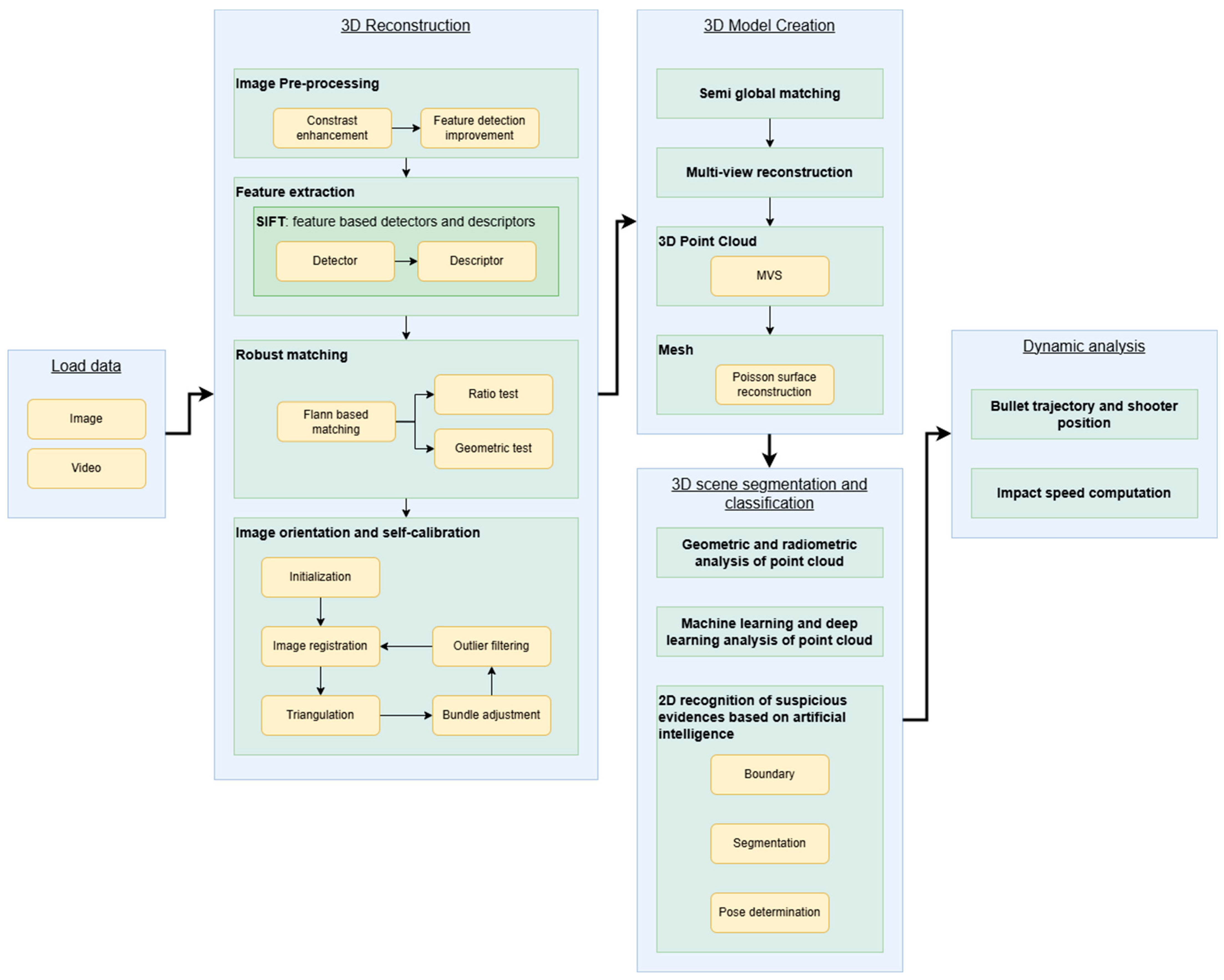
Figure 1. System architecture of the Law-Game Smart 3D Reconstructor, illustrating the modular pipeline from data input to dynamic forensic analysis.
Algorithms 18 00707 g001
Figure 2. User workflow within the tool, illustrating the operational steps from project creation to forensic analysis.
Algorithms 18 00707 g002
Figure 3. Tool component diagram.
Algorithms 18 00707 g003
Figure 4. Tasks for the reconstruction of 3D environments.
Algorithms 18 00707 g004
Figure 6. Matching algorithm comparison for (a) car accident scene images and (b) simulated crime scene images.
Algorithms 18 00707 g006
Figure 7. Visual comparison of point clouds generated by MVS, PMVS, and SMVS algorithms.
Algorithms 18 00707 g007
Figure 8. YOLOv8 semantic classification architecture. Dynamic analysis.
Algorithms 18 00707 g008
Figure 11. Deformation measurement protocol.
Algorithms 18 00707 g011
Figure 13. Sparse model of the car accident.
Algorithms 18 00707 g013
Figure 14. Three-Dimensional point cloud of the car accident.
Algorithms 18 00707 g014
Figure 15. Mesh of the car accident scenario.
Algorithms 18 00707 g015
Figure 16. (a) Semantic classification of 3D point clouds. (b) Semantic classification within images.
Algorithms 18 00707 g016
Figure 17. Form with the information of the vehicle of the car accident scenario.
Algorithms 18 00707 g017
Figure 18. Deformation measurements shown in the tool.
Algorithms 18 00707 g018
Figure 19. Impact speed estimation.
Algorithms 18 00707 g019
Figure 20. (a) Uploading images of the simulated crime scene. (b) Sparse model of the crime scene.
Algorithms 18 00707 g020
Figure 21. (a) Dense model of the crime scene. (b) Mesh of the crime scene.
Algorithms 18 00707 g021
Figure 22. (a) Point cloud semantic classification of the crime scene. (b) Semantic classification of images for the crime scene.
Algorithms 18 00707 g022
Figure 23. Bullet hole detection.
Algorithms 18 00707 g023
Figure 24. Bullets trajectories and shooter position estimation.
Algorithms 18 00707 g024
Table 1. Comparison of Dense Matching Algorithms by Execution Time and Point Cloud Density.
AlgorithmExecution TimeNumber of Generated 3D Points
MVS0.47 min5,427,919
PMVS12 min1,868,967
SMVS1.2 min4,029,451
Table 2. Features to describe points and their neighbourhood [112].
Features Definitions
Sum of eigenvalues λ i
Omnivariance λ i 1 3
Eigenentropy λ i ln ( λ i )
Linearity ( λ 1 λ 2 ) / λ 1
Planarity ( λ 2 λ 3 ) / λ 1
Sphericity λ 3 / λ 1
Change in curvature λ 3 / ( λ 1 + λ 2 + λ 3 )
Verticality (x2) π 2 a n g l e ( e i , e z ) i ϵ ( 0,2 )
Absolute moment (x6) 1 | Ν | p p 0 , e i   k i ϵ ( 0,1 , 2 )
Vertical moment (x2) 1 Ν p p 0 , e z k
Number of points Ν
Average colour (x3) 1 Ν c
Colour variance (x3) 1 Ν 1 ( c c ¯ ) 2
N: Neighbourhood, C: Colour channel.
Table 3. Prasad coefficients.
Categories Frontal Crash Side Impact Rear Impact
d0d1d0d1d0d1
Category 192.87569.06125.18511.6826.69504.90
Category 283.27544.31128.74531.7436.06679.43
Category 389.31621.16130.31550.6048.31626.68
Category 4128.68484.16100.09624.1642.64586.94
Category 5112.64504.9174.84694.4854.43569.06
Vans71.94931.7485.28615.500.000.00
Table 4. Camera calibration parameters of the car accident scenario.
f x 3857.97744003   p x
f y 3854.31291638   p x
c x 2247.15780393   p x
c y 1729.64177297   p x
k 1 0.06235381
k 2 0.03117001
fx/fy: focal lengths
cx/cy: principal point coordinates
k1/k2: radial lens distortion
Table 5. Deformation measurements.
Measurement Deformation
C10.446
C20.392
C30.315
C40.234
C50.185
C60.152
C70.136
C80.238
C90.286
C100.331
C110.334
C120.325
C130.322
C140.306
C150.209
C160.131
C170.076
C180.023
C190.339
C200.281
Table 6. Camera calibration parameters of the crime scene.
f x 2173.89614145   p x
f y 2174.278527   p x
c x 1919.51220484 p x
c y 1084.28286666 p x
k 1 0.00155018
k 2 0.00038535
fx/fy: focal lengths
cx/cy: principal point coordinates
k1/k2: radial lens distortion
Table 7. Bullet holes features.
Bullet Hole 1 Bullet Hole 2
Azimuthian impact angle24.4746°40.395°
Elevation impact angle0.264709°5.57001°
Horizontal directionalityRightRight
Ellipse length111 px151 px
Ellipse width267 px232 px
Cx2137 px1788 px
Cy1384 px1276 px
Cx/Cy: ellipse center
Table 8. Bullet holes positions and trajectories.
X Y Z V X V Y V Z
Bullet hole 10.515−1.749−0.481−0.9040.423−0.070
Bullet hole 2−0.769−1.772−0.490−0.7470.658−0.095
Disclaimer/Publisher’s Note: The statements, opinions and data contained in all publications are solely those of the individual author(s) and contributor(s) and not of MDPI and/or the editor(s). MDPI and/or the editor(s) disclaim responsibility for any injury to people or property resulting from any ideas, methods, instructions or products referred to in the content.