1. Introduction
Modern efforts toward highly automated production—commonly encapsulated under the label Industry 4.0 [
1,
2]—envision progressively autonomous control of technological processes with minimal human intervention. A major challenge in this context is the regulation and short-term forecasting of processes that unfold in unstable immersion media [
3,
4], such as turbulent gas—and hydrodynamic flows characteristic of chemical, petrochemical, biochemical, and related industries [
5,
6,
7,
8,
9]. Time series observed in these environments depart markedly from textbook notions of stationarity: they exhibit nonstationary variability, oscillatory and aperiodic trajectories of the system component, and strong low-frequency contamination in the noise. Such properties undermine the applicability of classical statistical analysis and forecasting techniques grounded in stationary white-noise assumptions.
A natural formalization begins with the generalized Wold decomposition,
but with components that diverge substantially from the classical case [
10]. In unstable processes, the system component
is oscillatory and aperiodic with multiple local trends—features consistent with deterministic or stochastic chaotic dynamics—while the noise component
is nonstationary, approximately Gaussian, with time-varying parameters and pronounced low-frequency behavior. In practice, practitioners obtain a provisional estimate of
using exponential smoothing or Kalman-type filters [
11,
12,
13]. These methods are attractive in online settings, yet the assumptions that guarantee their optimality are violated: stronger smoothing suppresses variance but introduces a phase delay harmful for extrapolation, while weaker smoothing reduces delay at the expense of high variance, rendering the output unsuitable for control [
14]. Prior to modeling, therefore, data must undergo sliding-window diagnostics for nonlinearity, nonstationarity, and approximate Gaussianity, followed by an assessment of whether the process is better described as dynamic or stochastic chaos [
15,
16]. Previous studies argue that stochastic chaos often provides the most faithful phenomenology for such signals, as uncertainty emerges from a combination of deterministic structure and stochastic perturbations [
17,
18].
Within these regimes, polynomial extrapolation—even over short horizons—functions only as a weak regressor or classifier. It captures local tendencies over limited look-ahead, yet exhibits pronounced delay relative to observed trajectories and rapidly loses directional accuracy as the forecast horizon grows, particularly when stochastic micro-trends dominate. In proactive control, however, operational requirements often reduce to the correctness of directional forecasts over short horizons, which motivates evaluating models by the frequency of correct directional decisions alongside mean-squared error (MSE). Empirical results from chaos-affected domains, including high-variability industrial data and financial markets, reveal weak inertia and abrupt trend inversions, both of which intensify the lag and overreaction characteristic of fixed-structure extrapolators.
To address these limitations, we adopt the multi-expert systems (MES) framework [
19,
20,
21,
22], in which a population of lightweight programmatic experts—each trained on a sliding window and defined by a structure S and parameters P—produces forecasts subsequently combined by a supervisory expert [
23,
24,
25]. MES exploits structural diversity to reduce variance and provides a natural pathway to online adaptation. Traditional boosting, which reweights experts to correct residual errors, offers a principled mechanism for allocating capacity where prediction is most difficult [
26].
From a statistical perspective, reweighting primarily targets residual variance while leaving structural bias from model misspecification unchanged; classical results on estimation and extrapolation make clear that no choice of weights can remove bias when the hypothesis class is inadequate [
27,
28]. In ensemble terms, this matches the weak-learner premise: base models must be at least slightly informative within a fixed class for a meta-learner to yield consistent gains [
29]. In chaotic time series, simple polynomial extrapolators frequently act as weak (or marginal) classifiers whose phase lag and trend errors persist under reweighting [
30]. Yet in contexts characterized by weak inertia and abrupt regime shifts, weight adaptation alone proves insufficient: if the expert pool itself is ill-suited to the prevailing regime (e.g., due to overly long windows or high polynomial orders), boosting cannot overcome this structural mismatch, and ensemble performance degrades [
31,
32].
This motivates adapting not only the weights of experts but also the pool itself. We therefore introduce evolutionary boosting, designed specifically for unstable and chaos-affected regimes. In this framework, experts are treated as ancestors whose “genomes” encode window length L and polynomial order p. Each generation applies variation and reproduction—small parameter adjustments, occasional strong mutations, and rare structural mutations that alter p—and selection that preserves the fittest survivors according to task-consistent criteria, with MSE serving as the primary criterion in our experiments, while directional accuracy is treated as an optional, application-specific complement. Because the best ancestors always remain eligible to reproduce, the evolutionary process is monotone non-worsening, while randomized mutations allow escape from poor local optima [
33,
34,
35,
36]. Numerical experiments on real monitoring data for turbulent gas-dynamic processes [
37] confirm that evolutionary boosting favors short-horizon experts (smaller L, lower p) that reduce MSE relative to single-model polynomial baselines; in contrast, indiscriminate increases in p degrade extrapolation by overfitting stochastic micro-trends rather than capturing meaningful system dynamics [
38,
39].
Recent research provides a broader context for this contribution. Surveys of data-stream learning and concept drift highlight the need for rapid online adaptation, including unsupervised and recurrent drift scenarios encountered in industrial monitoring [
40,
41]. Adaptive ensembles such as Adaptive Random Forests demonstrate how maintaining pools of learners with embedded drift detection can stabilize performance under evolving distributions, though typically within fixed model families [
42]. In parallel, deep-learning-based forecasting has advanced for nonlinear and chaotic sequences, from broad reviews to specialized architectures such as TCN–linear hybrids and chaos-aware priors, albeit with significant training overhead and sensitivity to horizon length and data quality [
43,
44,
45]. At the same time, evolutionary search has re-emerged as a practical tool for model configuration and hyperparameter optimization in nonstationary or computationally demanding environments [
46]. Our approach is aligned with these directions yet complementary: unlike deep architectures, it delivers short-horizon control through lightweight polynomial experts, and unlike purely weight-adaptive ensembles, it evolves the structure of the pool itself—window length and polynomial order—to mitigate structural lag under weak inertia and abrupt inversions, all within the MES architecture developed in this study.
2. Background
To describe unstable technological processes and the corresponding observation series produced by monitoring systems, it is natural to begin with the generalized Wold model, as originally justified in [
10]. While the additive two-component structure of the decomposition:
remains unchanged, the interpretation of the system and noise components differs substantially from the classical formulation. In the original Wold model, the system component is an unknown deterministic process relevant for control, and the noise component is generated by stationary white noise. For unstable technological processes, however, the generalized Wold framework is adopted with the same formal structure (1) but with components redefined as follows.
First, the system component is an oscillatory yet aperiodic process characterized by multiple local trends. These properties point to the relevance of models from the theory of dynamic chaos. Second, the noise component is a nonstationary stochastic process that can only be approximately described by a Gaussian model with time-varying parameters. In particular, its variations include local trends, and its correlation properties change significantly over time.
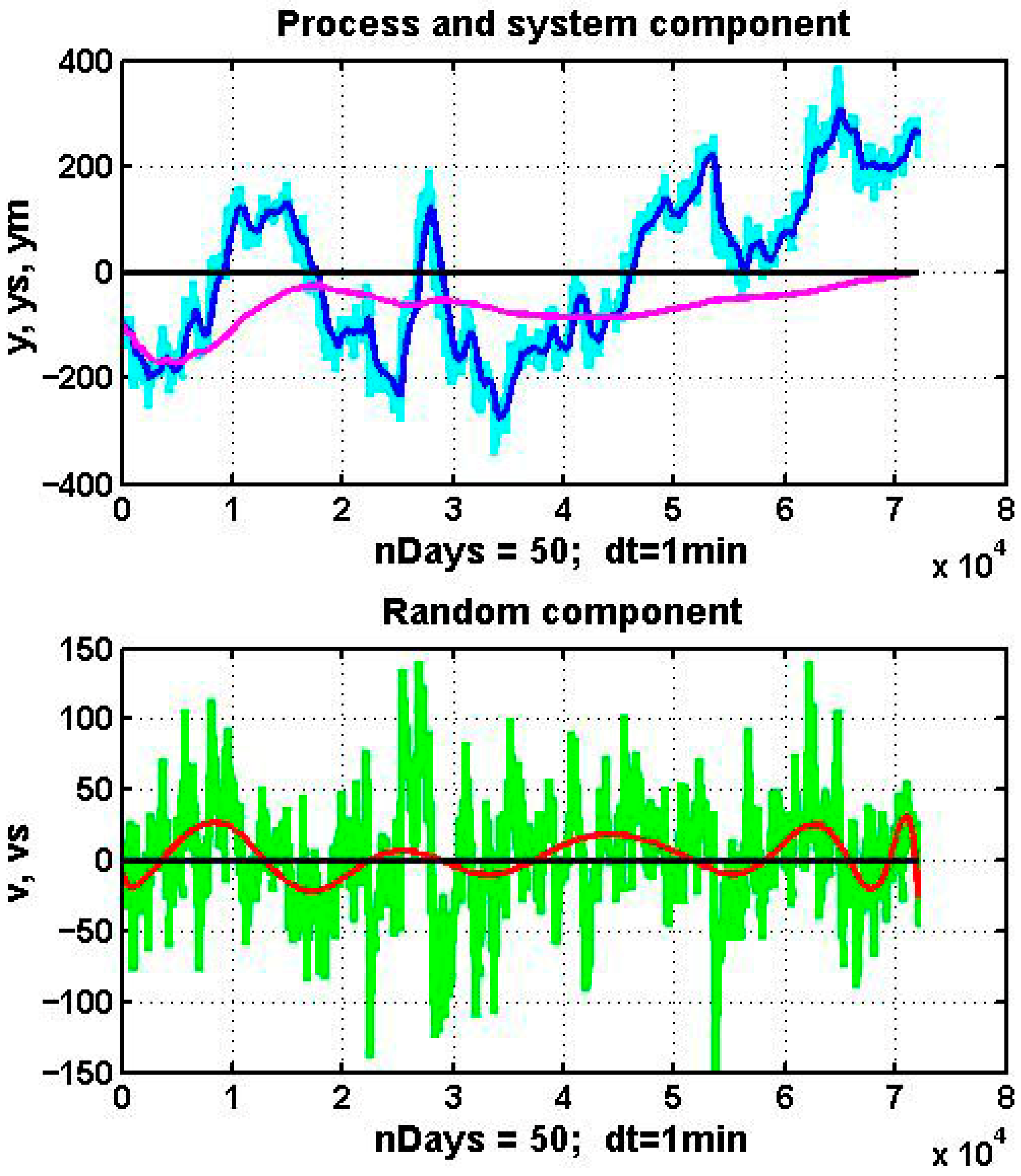
These features are illustrated in
Figure 1, which shows observation data for a normalized state parameter of an oil-refining process monitored over a 50-day period with sampling interval dt = 1 min. The upper panel displays the observed process (light blue line), a sequential mean estimate (magenta line), and the result of exponential smoothing (dark blue line). The lower panel shows the estimated noise component and its polynomial approximation of degree 15.
The observed process, represented by the light blue line, reveals stochastic local trends and evidence of scale invariance. To isolate the system component, both the sequential mean estimate:
shown in magenta, and the exponential smoothing filter [
11]:
shown in dark blue, were applied, where
. In this example, α = 0.002.
The sequential mean estimate (2), due to its high inertia, is clearly unsuitable as a basis for forecasting or control. More dynamic algorithms such as (3), modifications of the Kalman filter [
12,
13,
14], and related approaches are more appropriate. Reducing the gain parameter α improves smoothing quality but simultaneously increases the bias of the estimate, manifested in the figure as a temporal lag.
The noise component
, defined as the difference between the raw observations and the estimated system component, is plotted in green in the lower panel of
Figure 1. Its polynomial approximation, obtained by least squares with degree p = 15, is shown in red:
where coefficients
are estimated by ordinary least squares. As is evident, the approximating curve, like the system component, is oscillatory and aperiodic. The presence of a pronounced low-frequency component indicates that assumptions of independence and stationarity are violated. Increasing the smoothing gain in (3) effectively transfers more of the low-frequency variation into the system component
. However, the resulting system estimate is too noisy and highly variable to be useful for forecasting or decision-making.
Thus, the real data produced by monitoring unstable systems exhibit a complex structure that reflects both the dynamic characteristics of the underlying processes and the statistical properties of the raw observations. Deviations from the assumptions of classical models can easily lead to substantial forecast errors and, in turn, to reduced effectiveness of control decisions. For this reason, machine learning applications in such domains must include a stage of preliminary data analysis, typically performed on a sliding observation window of limited length. This diagnostic stage should be complemented by retrospective studies on longer horizons, aimed at establishing fundamental empirical properties of the monitored signals.
In practice, such analysis involves sequential testing of hypotheses regarding nonlinearity, nonstationarity, and Gaussianity. As a final step, one examines whether the observed series is more appropriately described by models of dynamic chaos or stochastic chaos. This task is especially challenging and remains an active subject of research [
15]. Prior studies [
3,
16,
17,
18] suggest that the concept of stochastic chaos provides the most complete description of the dynamics of unstable systems. To enhance stability and predictive accuracy under such conditions, recent work has proposed the use of multi-expert systems [
19,
20,
21,
22]. This approach overlaps conceptually with ensemble methods in machine learning [
23,
24,
25,
26]. The present study develops a specific realization of a multi-expert system based on an evolutionary boosting algorithm.
2.1. Linear Extrapolation as a Weak Short-Horizon Forecaster for Chaotic Processes
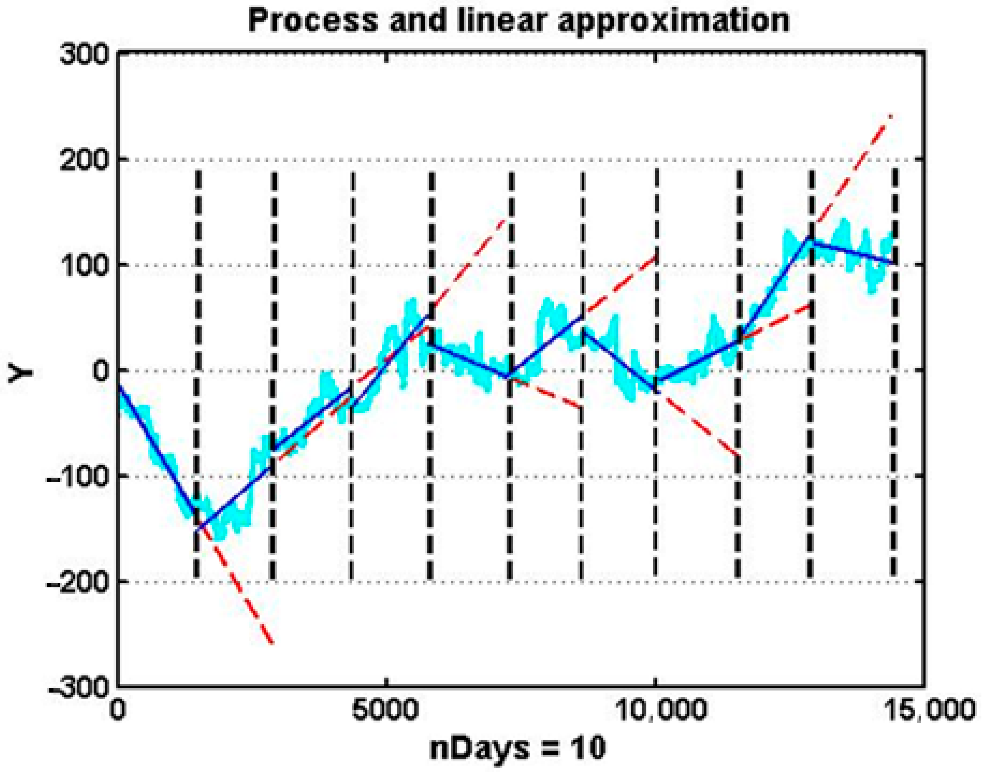
To illustrate the limitations of conventional forecasting techniques in chaotic environments, we consider the task of predicting the state parameter of an unstable technological process using the simplest form of polynomial extrapolation—a linear predictor. The training set is defined as a sliding observation window of length L = 1440 one-minute samples, corresponding to a full calendar day:
Within each window, the observed sequence is approximated by a first-order polynomial model,
where
are estimated by ordinary least squares [
27,
28]. The extrapolated forecast over a horizon of τ = L steps (i.e., one day ahead) is then obtained directly by substitution:
.
Figure 2 presents a representative example based on centered variations of gas-dynamic flow density observed over a 10-day interval. Visual inspection reveals a critical deficiency: out of nine consecutive forecasts, only a minority correctly reproduce the sign of the actual trend, indicating low directional reliability. Extending the analysis to a longer interval leads to similarly modest directional reliability. Such performance falls substantially below the level required for operational control, particularly in proactive decision-making settings where trend direction is often more relevant than absolute error.
From the standpoint of machine learning theory, this behavior identifies the linear extrapolator as a weak short-horizon forecaster: a predictor that provides slightly better than random accuracy but cannot independently support robust forecasting under stochastic chaos. While it captures broad linear tendencies, its inability to adapt to abrupt regime changes and micro-trends renders it unsuitable as a standalone forecasting tool for unstable technological processes.
2.2. Short-Horizon Forecasting with Linear Extrapolators
A natural question arises as to whether linear extrapolators may retain practical value when applied over very short horizons. To investigate this, we consider the forecasting of an unstable technological process using a sliding training window of length L = 120 one-minute observations.
Figure 3 illustrates the original chaotic process together with its forecast over a horizon of τ = 3 min within a single day.
The evaluation results confirm the limited utility of this approach: The root mean squared error (RMSE) was approximately 9.22, while the mean absolute error (MAE) was approximately 6.79 (computed for the case shown in
Figure 3). Even in this short-horizon setting, forecasting accuracy is unsatisfactory. Beyond random dispersion, the forecasts reveal a systematic bias manifested as a temporal lag relative to the observed process.
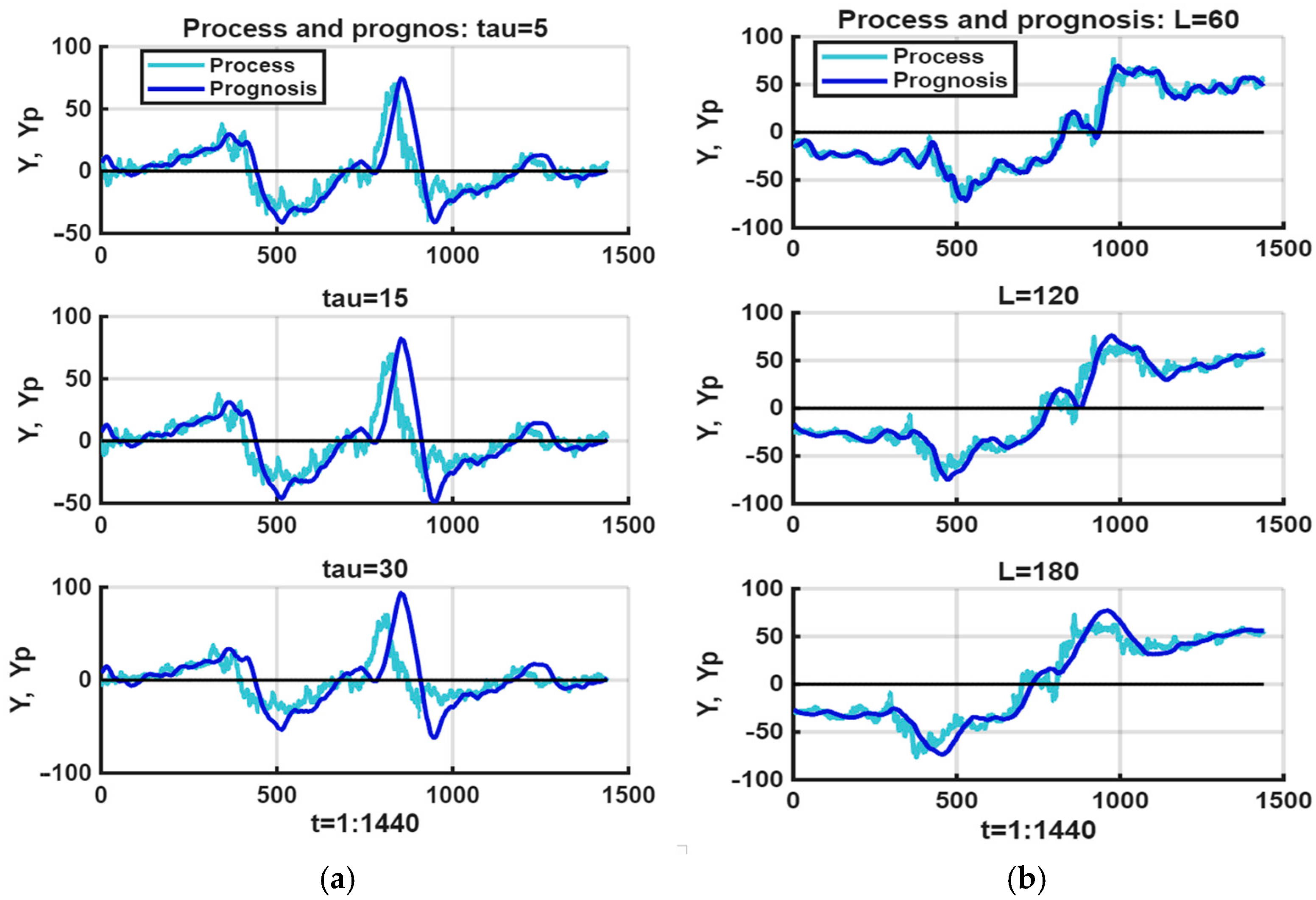
To further illustrate this effect,
Figure 4 compares the observed process (green line) with short-horizon linear forecasts (blue line) for different training-window lengths, L = {60,120,180}, and forecast horizons, τ = {5,15,30}. As expected, increasing L improves smoothing quality but simultaneously exacerbates the lag in forecasted values. Likewise, extending τ markedly increases the temporal delay, further degrading predictive adequacy.
These findings demonstrate that although short-horizon linear extrapolation can capture coarse local tendencies, its inherent bias and delay significantly limit its effectiveness in chaotic environments. This motivates the exploration of alternative models and ensemble-based techniques better suited for unstable processes.
2.3. Polynomial Extrapolation Beyond the Linear Case
A natural extension of the linear extrapolation approach is to employ higher-order polynomial models. According to the Weierstrass approximation theorem, any continuous function on a finite interval can, in principle, be approximated with arbitrary accuracy by sufficiently high-order polynomials. However, such approximation guarantees do not directly translate into reliable forecasting, especially in the context of unstable and chaotic processes.
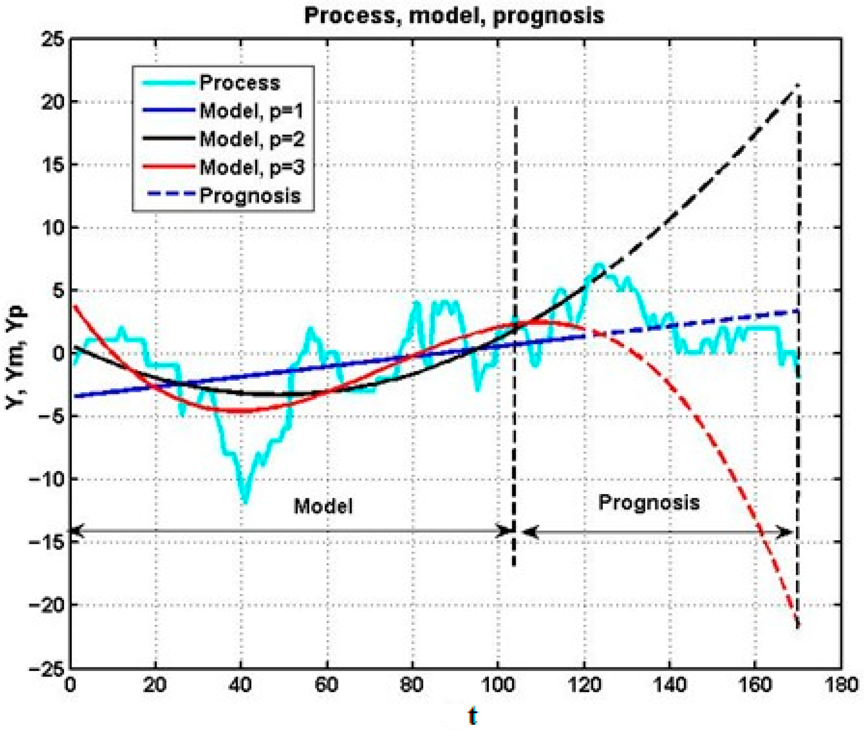
Figure 5 illustrates this limitation with forecasts of a nonstationary stochastic process using polynomials of degree 1, 2, and 3. While higher-order polynomials more closely interpolate the historical segment, they simultaneously introduce substantial forecast error. In fact, increasing the polynomial order leads to overfitting of local stochastic fluctuations, degrading predictive adequacy. Thus, in chaotic immersion environments, nonlinear polynomial models also behave as weak short-horizon forecasters.
Nevertheless, polynomial extrapolators retain some utility for short-horizon forecasts. As seen in
Figure 6, predictive adequacy is limited to horizons of no more than 15–20 steps. In practice, such horizons may be sufficient for many industrial processes: for instance, a lead time of τ = [
10,
20] min can often provide actionable guidance for corrective control.
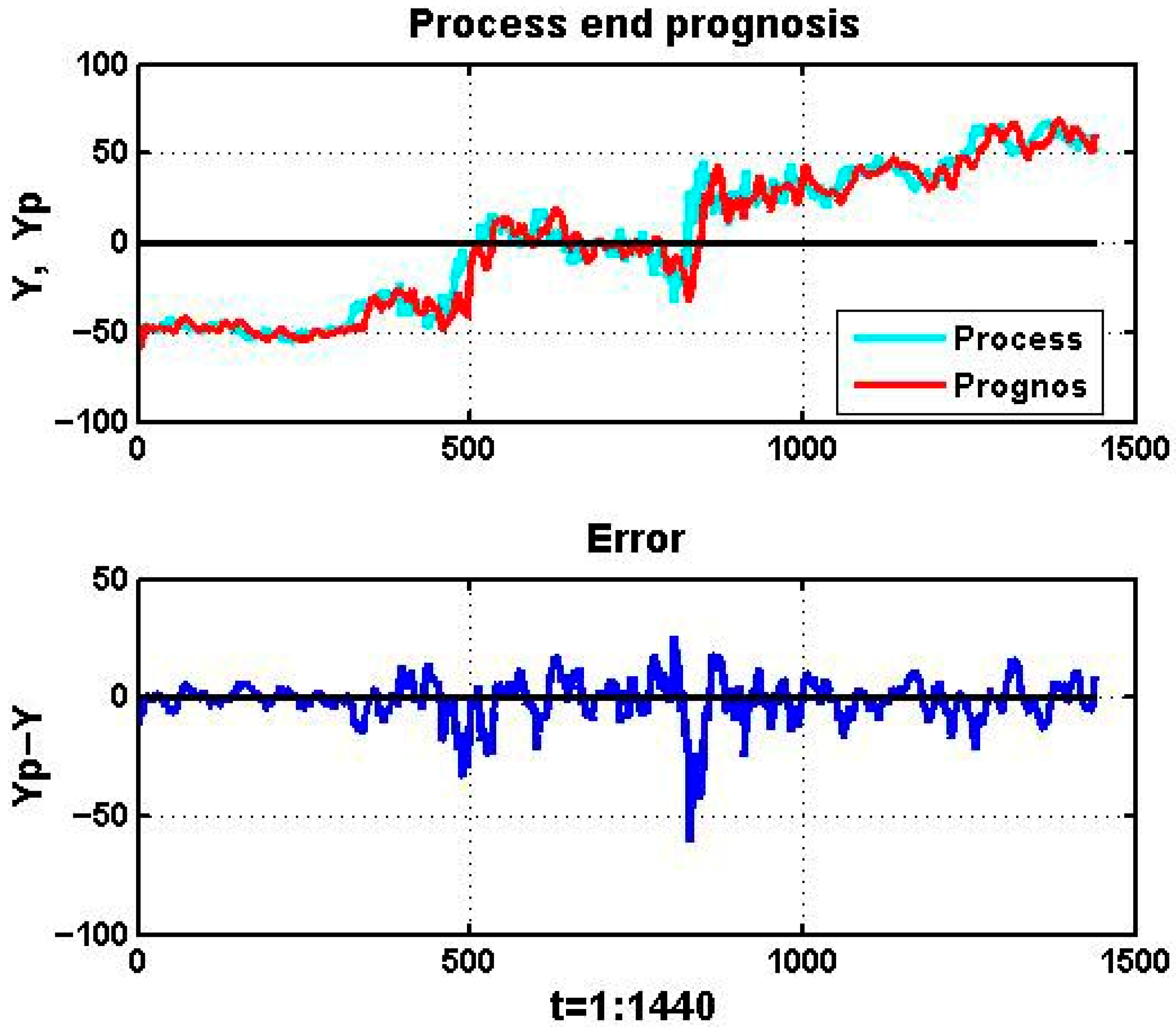
To illustrate this point,
Figure 6 presents results for a 24-h observation interval with training window L = 50 and forecast horizon τ = 20. The observed process is shown in blue, while red curves denote forecasts. The lower panel reports the forecast error, defined as
The forecast trajectory clearly exhibits a systematic bias, appearing as a temporal delay relative to the observed process.
Table 1 summarizes forecast quality metrics—MSE, bias, and total squared error—for polynomial orders p = 1, …, 5.
These results indicate that no monotone reduction in forecast error is achieved as p increases. Instead, forecast accuracy remains highly sensitive to the local dynamics of the observed segment. A similar ambiguity arises with respect to the size of the training window.
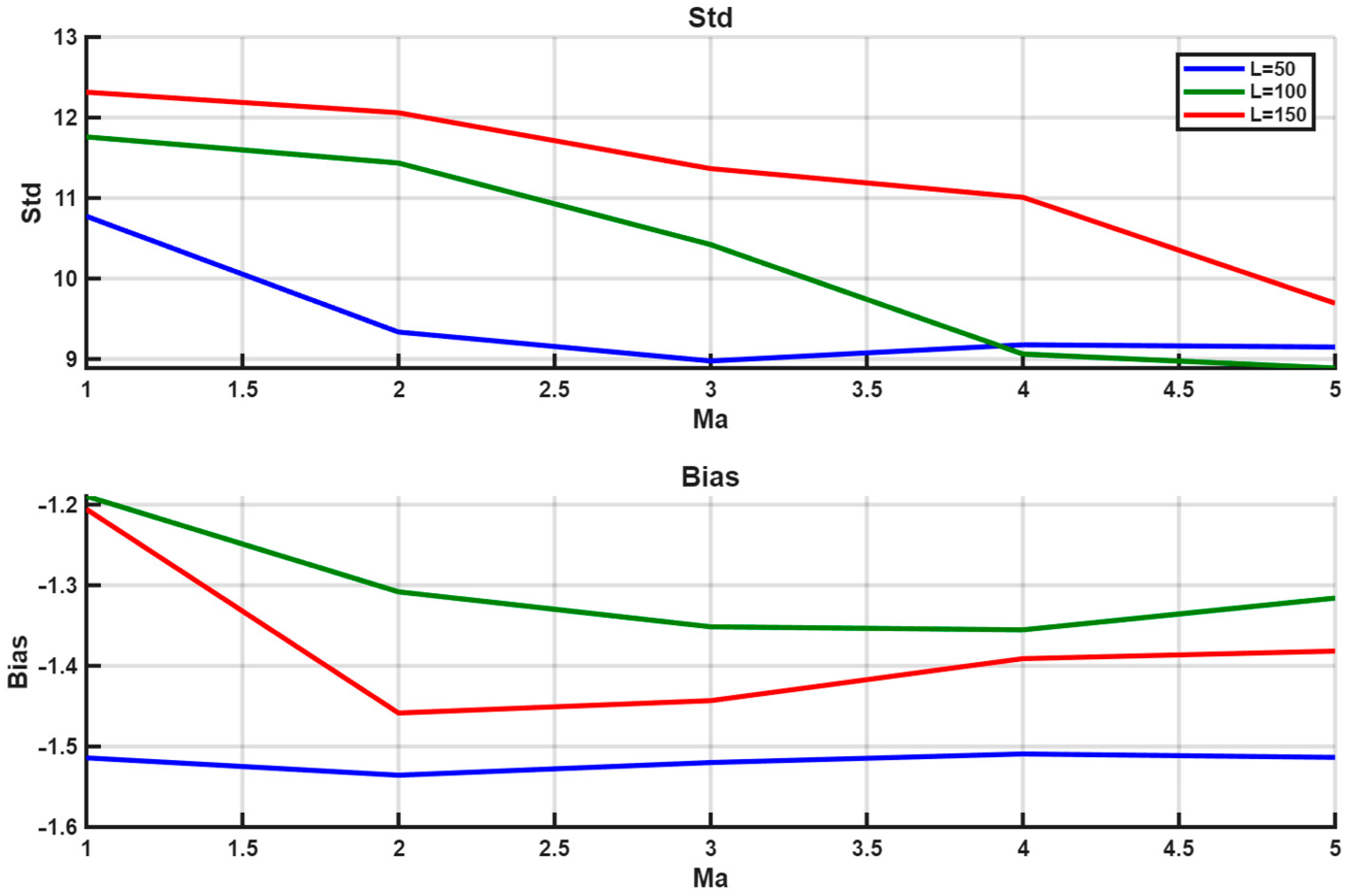
Figure 7 demonstrates how forecast error and bias vary with polynomial order for different window lengths L = {50,100,150}.
For
Figure 6 and
Figure 7 and
Table 1 we report the standard deviation of the error (σ) and the bias; the mean squared error satisfies
. In
Section 4 we report MSE for the evolutionary runs.
Taken together, these findings show that higher-order polynomial extrapolators do not consistently improve forecast performance under stochastic chaos. The high variability of results underscores the structural limitations of single-model extrapolation. To mitigate these weaknesses, the next section introduces a multi-expert system (MES) framework, which integrates multiple weak forecasters into a stronger collective forecasting mechanism.
2.4. Multi-Expert Forecasting for Unstable Technological Processes
To overcome the limitations of single-model extrapolation, we now formalize the problem of multi-expert forecasting for unstable technological processes. In the multi-expert systems (MES) framework, each programmatic expert (PE)
is defined by a forecasting algorithm of structure S and parameters P, and implements the mapping.
where
is the sliding training window (5),
—the current observation, and
—the forecast value at horizon τ.
The simultaneous operation of m experts produces, at each time step, a collection of forecasts:
The central task of MES is to construct a supervisory expert that aggregates these partial solutions into a terminal forecast of higher efficiency:
subject to
Here, efficiency
depends on the practical context. In proactive control settings, accuracy metrics such as MSE or MAE are appropriate. In other applications, however, directional correctness of forecasts may suffice. Specifically, a forecast is considered correct if the trend
matches the posterior trend of the realized process:
so that
If, among n forecasts, m
+ satisfy condition (10), then the efficiency of the expert is expressed as
This framing can be cast as a classification view when decision-making reduces to trend direction [
29,
30]: experts may be weak classifiers when
, or strong classifiers when
. The optimal expert is then defined as
In practice, however, criterion (12) is rarely achievable. Different experts prove more effective across different nonstationary intervals, and most individual PEs remain weak classifiers overall. Consequently, the central challenge is to design MES architectures in which the aggregation of weak classifiers yields strong solutions satisfying the task-specific adequacy criterion .
In this study, the aggregation mechanism is implemented through a variant of the boosting algorithm, grounded in the general principles of ensemble machine learning [
26]. This approach provides a systematic way to enhance weak classifiers into a robust forecasting system for unstable and chaos-affected processes.
3. Proposed Framework
The goal of the proposed framework is to construct a strong forecasting classifier from a population of weak polynomial extrapolators (6), aggregated by a supervisory rule (8). To this end, we introduce evolutionary boosting, an ensemble methodology that integrates boosting with evolutionary modeling to address the challenges of chaotic and weakly inertial dynamics.
3.1. Motivation
Classical boosting algorithms belong to supervised ensemble learning and are designed to sequentially train and combine weak classifiers in order to form a strong classifier. Early approaches based on recursive dominance [
24] lacked guarantees of effectiveness. Adaptive boosting (AdaBoost) introduced the idea of weight correction, dynamically reassigning weights to weak classifiers, and achieved promising results. This principle of adaptive weight adjustment inspired numerous variants—LPBoost, TotalBoost, BrownBoost, MadaBoost, LogitBoost, among others [
25,
26].
However, for unstable processes with chaotic dynamics, these methods fail [
31,
32]. Rapid and abrupt trend changes do not allow sufficient time for feedback loops to reassign classifier weights. As a result, ensemble adaptation lags behind the underlying dynamics. This motivates a shift from weight-based adaptation to structural adaptation of the expert pool, where both parameters and structures of experts evolve.
3.2. Evolutionary Boosting in the MES Framework
The evolutionary boosting procedure is formulated within the multi-expert system (MES) paradigm [
19]. Consider a set of ancestor experts
each defined by a forecasting algorithm structure S and parameter set P, so that
Forecasting efficiency
is measured by the similarity between predictions and retrospective monitoring data of the observed process.
The framework introduces two nonlinear operators:
Here, descendants
are generated by modifying ancestor experts, with
denoting the breeding coefficient. The combined set of
ancestors and
descendants defines a generation of size
The total population of a generation is:
- 2
Selection
From generation
, a subset of
fittest experts is selected as survivors for the next generation
with experts ranked by decreasing efficiency. We use elitism (the best individual is retained unmodified each generation), which guarantees a monotone non-worsening error trajectory. Starting from a base expert
), the process iterates:
Although global optimality is not guaranteed, this iterative scheme ensures monotone non-worsening, since the best ancestors always remain eligible to reproduce.
3.3. Convergence and Regularization
The evolutionary optimization process is convergent by design, because the best-performing experts are preserved across generations. However, convergence speed is typically comparable to that of stochastic search, due to the randomness of modifications. To accelerate convergence, one may allow the breeding coefficient
to vary with ancestor efficiency:
so that stronger ancestors produce more descendants. This mechanism is expected to increase convergence speed but requires further empirical validation. Other regularization strategies may also be considered to balance exploration and exploitation.
3.4. Mechanisms of Variation
Variation is implemented through randomized modifications to expert parameters and structures, chosen from the following set:
Small incremental changes—single-parameter adjustments (up to 10–20% of its value), chosen by random sampling (Monte Carlo analogy).
Strong parametric mutations—larger parameter changes (30–50%), applied occasionally (≈0.1 probability), enabling broader exploration.
Structural mutations—very rare events (≈0.01 probability) that modify the forecasting algorithm structure (e.g., changing the order ).
While multi-parameter updates are possible, they typically produce outliers far from the optimization trajectory and rarely survive selection. Nevertheless, strong and structural mutations are preserved to avoid premature convergence to local optima.
Because of the stochastic nature of variation, the evolutionary process operates beyond strict developer control, both at the parameter and structural levels. This open-ended evolution is advantageous: it allows the discovery of unexpected solutions and adheres to the principle of incomplete or open decisions, where each generation retains not a single best expert but a set of high-performing candidates.
This property is crucial in chaotic immersion environments, where diverse intermediate solutions may ultimately form the evolutionary chain leading to superior forecasting performance. By maintaining population diversity, evolutionary boosting reduces the risk of overfitting to transient patterns and enhances resilience under abrupt regime shifts.
3.5. Baseline Genome and Mutation Rates
The ancestor genome was selected based on domain diagnostics and preliminary experiments. Sliding-window lag–variance analysis of the one-minute time series with a 20-min horizon () indicated that windows in the range keep the cross-correlation lag of the fitted trend below 8–10 min while preventing variance inflation. Shorter windows () increased RMSE by 6–12% due to noise following, whereas longer windows () introduced phase delay and reduced directional accuracy.
Starting from mitigates premature over-reaction to stochastic micro-trends; higher curvature, if beneficial, can emerge later through structural mutation of . This initialization is conservative with respect to the best genomes subsequently observed around and , allowing evolution to proceed toward empirically favorable regions of the search space.
We employ frequent weak variations (probability 0.8; ±10–15% of a parameter) to exploit local improvements, occasional strong mutations (0.1; ±45–50%) to escape shallow basins, and rare structural mutations (≈0.01) to alter .
Let
denote the number of descendants per survivor and
the number of survivors per generation. The expected number of structural events per generation is
Under typical settings (, , ), this yields —roughly one polynomial-order change every one to two generations, sufficient to explore without destabilizing convergence.
4. Experiments
To validate the proposed evolutionary boosting framework, we consider the short-horizon forecasting problem introduced in
Section 3. The forecast horizon is τ = 20 samples (minutes), i.e., predictions 20 steps ahead. The target process is a turbulent gas-dynamic flow parameter observed over an interval of 1440 one-minute samples (one calendar day).
In the evolutionary framework, each programmatic expert (PE) is defined by a genome , where L is the size of the sliding training window and p is the order of the polynomial extrapolator. The initial ancestor expert was set as , i.e., ≈2-h (130 min) window and a linear extrapolator.
The admissible ranges and probabilities of genome modifications are summarized in
Table 2 and
Table 3, which show how weak, strong, and structural mutations affect the values of L and p. This design allows balancing incremental fine-tuning (weak variations) with occasional disruptive changes (strong and structural mutations).
The forecast horizon was fixed at τ = 20 min, which is adequate for operational decision-making in technological systems. The predictive quality of each PE was assessed using mean squared error (MSE):
This choice allows consistent comparison across structurally different experts and directly reflects industrial requirements for minimizing deviations in parameter forecasts.
We examined how the ancestor genome influences convergence and final accuracy.
Ten evolutionary trajectories with distinct random seeds were launched for each initialization, fixing
. For each run we recorded (i) the best mean-squared error (MSE) and (ii) the generation
at which the MSE first reached ≤1% of its final value (“time-to-plateau”). Reported values are medians across seeds (see
Table 4).
These results indicate that (i) final accuracy is robust to sensible ancestor choices, and (ii) extreme window lengths affect mainly rather than the achievable MSE. Using as the baseline is therefore justified, since the evolutionary process reliably introduces curvature when it improves fitness.
Then we ablated the weak, strong, and structural mutation probabilities while keeping other settings fixed. Median final MSE and
were computed across ten seeds; the results are summarized in
Table 5.
As shown in
Table 5, the mutation probabilities exert a predictable but moderate influence on both convergence speed and attainable accuracy. Runs with a non-zero structural-mutation rate consistently outperform those without one: disabling structure mutations (row 2) traps the evolution at
and raises the final MSE by ≈17%. Increasing the rate beyond ≈0.02, however, introduces excessive order changes that slow stabilization. Hence, values in the 0.01–0.02 range achieve the best balance between exploration and stability. Adjusting the weak-to-strong mutation ratio primarily affects early dynamics—more frequent strong mutations accelerate initial progress but do not improve final accuracy—confirming that the algorithm’s long-run performance is robust to moderate changes in these parameters.
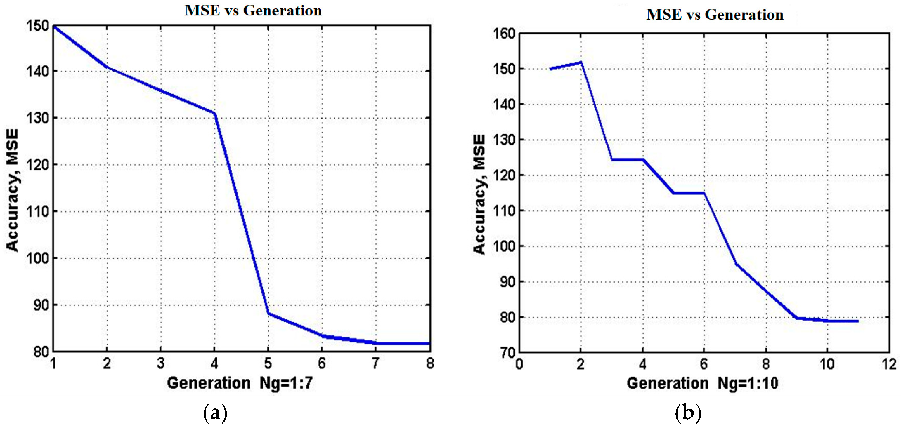
Figure 8 illustrates the convergence of MSE values across generations, with corresponding results summarized in
Table 6. Error reduction is steep during the first few generations and then stabilizes. For example, the 7-generation run converged to an expert with genome
, while the 10-generation run produced a superior result with
.
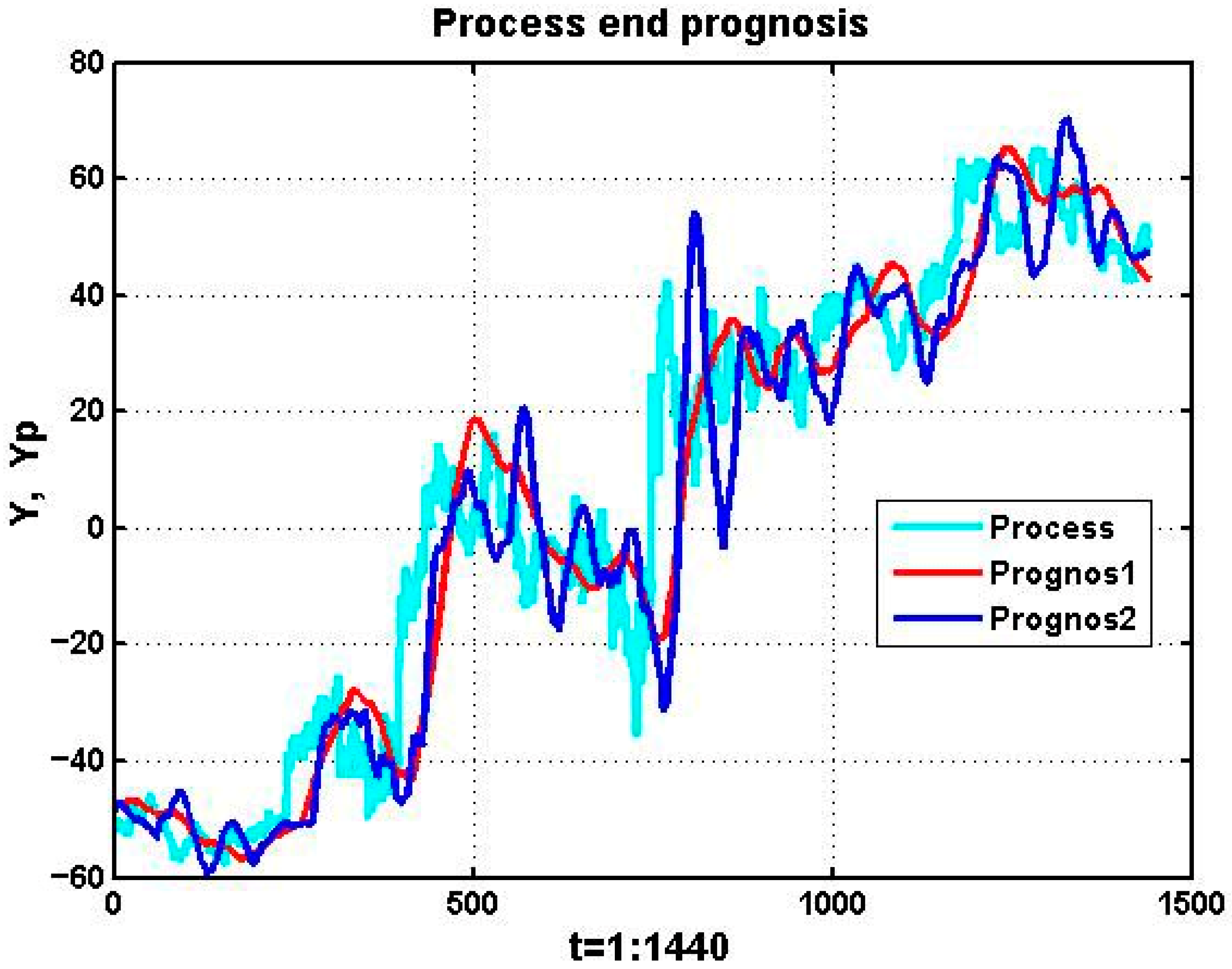
The influence of polynomial order is illustrated in
Figure 9. First-order models (red line) are stable but lag behind the process trajectory, while third-order models (blue line) capture local fluctuations but also overreact to noise. This trade-off explains why the best-performing genomes in
Table 6 tend to feature moderate orders (p = 3–5), balancing adaptivity and robustness.
To contextualize the advantages of evolutionary boosting (EB), we conducted a comparative experiment with three representative methods evaluated on the same dataset, forecast horizon, and metrics. The baselines include:
Adaptive Random Forest (ARF)—a streaming ensemble designed for non-stationary data and concept drift;
Temporal Convolutional Network with Linear head (TCN-Linear)—a deep hybrid suited for chaotic temporal dependencies;
Exponential Weighted Moving Average (EWMA)—a simple operational baseline for short-term smoothing.
All models use identical one-minute data and a short-horizon setup with
min. Each model receives the last
observations as input. EB evolves both
and
through structural adaptation (
Section 3.4 and
Section 3.5), whereas ARF and TCN-Linear directly consume a fixed window (TCN employing a causal 1D convolutional stack).
Performance is assessed by mean squared error (MSE), directional accuracy (DA; fraction of correct directional predictions per Equations (10) and (11)), and inference time per forecast (CPU, single thread). Ten random seeds were used; results are reported as medians across runs. The EB row reproduces the best configuration from
Table 6.
Baseline configurations are as follows:
ARF: 10 Hoeffding trees, ADWIN drift detector, unconstrained depth, auto-binning for nominal features.
TCN-Linear: 5 temporal blocks, kernel = 3, dilations = (1, 2, 4, 8, 16), linear output head for ; 20 epochs with MSE loss and early stopping.
EWMA: smoothing factor optimized on a rolling validation grid (); forecasts formed by -step continuation of the filtered trend.
Directional accuracy computed per Equations (10) and (11) at
. Inference time measured per single forecast on a standard CPU (training excluded). EB’s MSE (78.9) corresponds to the best genome reported in
Table 6. Inference time is the median wall-clock per single forecast on a single-thread CPU, batch size = 1, training excluded.
As summarized in
Table 7, EB achieves the lowest MSE and highest directional accuracy while maintaining low inference latency. At inference, EB outputs the best survivor (top-1) per generation; ensemble averaging over a small elite (e.g., top-3) yields similar results with <3 ms latency. The TCN-Linear hybrid narrows the error gap but incurs a higher computational cost. ARF demonstrates stability under concept drift but exhibits a residual phase lag at τ = 20. The EWMA baseline is computationally efficient but suffers from smoothing bias and reduced directional precision. Collectively, these results attribute EB’s advantage to its structural adaptability—the joint evolution of L and p beyond mere weight updates—effectively mitigating phase lag without overfitting stochastic fluctuations. This is consistent with the convergence patterns in
Table 6 and the concentration of best genomes around L ≈ 110–120 and p = 3–5.
5. Discussion
The results of this study highlight the fundamental limitations of classical forecasting approaches when applied to processes governed by stochastic chaos. Traditional statistical models rely on assumptions of stationarity, ergodicity, and white-noise perturbations, conditions that are consistently violated in unstable immersion media. The monitored time series in our experiments exhibit oscillatory and aperiodic dynamics with weak inertia and frequent trend reversals, while the noise component is strongly nonstationary and characterized by low-frequency contamination. Under such conditions, estimators lose their desirable properties of unbiasedness, efficiency, and consistency, and even short-horizon linear extrapolators perform only as weak learners. Their forecasts achieve directional accuracy only marginally above chance and are further undermined by a systematic phase lag that reduces their usefulness for proactive control.
Against this background, the proposed framework of multi-expert systems provides a natural solution by combining a population of weak learners through a supervisory expert. The originality of the approach lies in the use of evolutionary boosting, which differs from conventional boosting techniques by not only reweighting a fixed set of learners but also adapting the structure of the expert pool itself. Each expert is defined by its genome, consisting of the training-window length and polynomial order. These parameters embody the bias–variance trade-off inherent in chaotic forecasting: shorter windows reduce lag but increase variance, while higher polynomial orders increase responsiveness at the cost of noise amplification. The evolutionary operators of variation, mutation, and selection allow the system to refine promising configurations while also escaping local minima, something that weight adaptation alone cannot achieve.
The numerical experiments confirm the effectiveness of this strategy. Across multiple one-day intervals, evolutionary boosting consistently reduced mean squared error by approximately 45 to 48 percent compared with the baseline ancestor model. The convergence curves demonstrated that once an effective configuration appeared, it was preserved across generations, producing a monotone non-worsening trajectory. Importantly, the best experts consistently clustered around shorter training windows of about 110 to 120 min and moderate polynomial orders between three and five. These settings represent an empirical compromise that reduces the phase lag of linear fits without fully succumbing to the volatility of high-order models.
Figure 9 illustrates this trade-off directly: first-order extrapolators yield smooth but lagging trajectories, while third-order models react more quickly but overfit stochastic fluctuations, resulting in oscillatory forecasts. The evolutionary process naturally converged to intermediate orders where responsiveness and stability are balanced.
The role of mutation diversity was also apparent. Small, frequent variations of the window length led to incremental improvements, but major gains occurred when structural mutations introduced new polynomial orders. This confirms that structural mutation is crucial for avoiding premature convergence and for adapting to abrupt regime shifts in the underlying process. Occasional strong mutations on the window size further contributed to exploration, allowing the algorithm to avoid overcommitting to overly inertial solutions. Taken together, these mechanisms explain the consistent error reduction and directional improvement documented in our experiments.
From an operational perspective, the results suggest that evolutionary boosting is particularly well suited for proactive control in unstable technological processes, where decision value depends more on the correctness of short-horizon directional forecasts than on long-horizon accuracy. By continually adjusting both the weights and the structural parameters of its experts, the system provides reliable short-term predictions that remain responsive to rapid environmental changes. Moreover, because the evolutionary process always retains the best-performing ancestors, the method has an anytime character: it can be stopped at any generation without performance deterioration. Computationally, the speed of convergence depends on mutation stochasticity, but adaptive breeding coefficients and carefully managed structural mutation rates can accelerate progress without destabilizing the population.
In relation to other ensemble methods, evolutionary boosting extends the principles of boosting and bagging by introducing structural adaptivity into the expert pool. Unlike AdaBoost, which struggles with abrupt inversions due to slow reweighting dynamics, evolutionary boosting can replace ill-suited learners with structurally better ones. Compared with deep learning architectures designed for chaotic sequences, the approach emphasizes lightweight, interpretable experts that adapt rapidly without requiring extensive retraining. These advantages make it complementary to more complex models, which could in future be incorporated as additional species within the evolutionary pool.
Sensitivity analyses (
Table 4 and
Table 5) confirm that the algorithm’s performance is robust to the initial genome: different plausible starting points converge to comparable MSEs, with variation mainly in time-to-plateau rather than attainable accuracy. Crucially, a non-zero structural-mutation rate (≈1–2%) is required to escape
basins; disabling structural mutation raises final MSE by ≈17% in our data, underscoring the role of structural adaptivity in chaotic regimes. Across ablations, optimal genomes consistently clustered around
and
, consistent with the bias–variance trade-off and the converged experts reported in
Table 6.
A comparative evaluation against representative stream-learning (ARF), deep hybrid (TCN-Linear), and operational (EWMA) models further substantiates the robustness of evolutionary boosting. EB attains the best overall trade-off among accuracy, directional reliability, and inference efficiency at . EB’s advantage arises from structural adaptivity—the capacity to evolve both the effective window length and polynomial order —which minimizes phase lag under weak inertia without over-fitting transient micro-trends. By contrast, ARF’s fixed hypothesis family retains residual lag at , and TCN-Linear architectures depend on deeper convolutional stacks to stabilize chaotic dynamics, thereby increasing inference cost. Importantly, EB’s experts are transparent and interpretable: directly maps to an equivalent process time constant and to local curvature, enabling diagnostic insight and safer control-loop integration. Combined with the algorithm’s anytime property—retaining best survivors across generations—these traits make EB a practical, auditable, and latency-efficient framework for proactive industrial control, where timely and directionally accurate decisions are paramount.
Recent developments at the intersection of optimization [
47], AutoML, and large language models (LLMs) open promising directions that complement our lightweight EB framework. Notably:
Model merging and multi-objective consolidation for pretrained models [
48].
LLM-mediated transfer of design principles in neural architecture search [
49].
Robust and explainable algorithm selection [
50].
Multimodal integration combining textual and numerical signals for optimization [
51].
LLM-guided black-box search and evolutionary strategies [
52,
53] introduce generic mechanisms for steering complex searches under multiple objectives.
Within our context, such advances can operate above the expert pool—as meta-controllers that provide priors and scheduling strategies for EB—while preserving EB’s core deployment properties: short-horizon responsiveness, interpretability, and CPU-level latency.
Concretely, three non-intrusive integration hooks can be envisioned. The first integration involves LLM-guided priors for the ancestor genome. Using basic diagnostics such as lag–variance profiles at , an LLM can propose priors over and (for example, , ) together with initial mutation probabilities. Evolutionary boosting can then perform the actual search, potentially reducing the time-to-plateau while preserving its internal selection dynamics.
A second integration concerns LLM-assisted algorithm selection, or the explainer–selector approach. A concise, auditable prompt can transform sliding-window descriptors into a recommendation to retain polynomial experts or to augment them with compact state-space experts. This selector functions offline so that the per-forecast inference process remains unchanged.
The third integration relates to multimodal gating. Textual operational notes or log entries may be embedded once per interval and employed to modulate the structural-mutation probability, for instance with higher values during maintenance regimes. This mechanism likewise operates outside the per-forecast path and therefore does not affect runtime efficiency.
These integrations treat LLMs as planning tools rather than inference engines, aligning with our goal of maintaining EB’s transparency and millisecond-scale latency while extending its adaptability to the emerging LLM-driven optimization paradigm.
The present study is not without limitations. We deliberately focused on univariate polynomial extrapolators in order to isolate the dynamics of the evolutionary mechanism and to provide results that could be visualized transparently. While this choice clarified the trade-off between lag and overreaction, it does not capture the full potential of richer base learners such as state-space models, kernel regressors, or compact neural networks. Furthermore, the experiments were confined to a 20-min horizon and to particular industrial data sets; generalization to other horizons, noise structures, and exogenous factors remains to be established. Nevertheless, the results provide strong evidence that evolutionary boosting can transform weak polynomial extrapolators into a robust strong classifier for chaotic short-term forecasting tasks.
6. Conclusions
This work addressed short-horizon forecasting for unstable technological processes—signals shaped by stochastic chaos where stationarity assumptions fail and fixed-structure predictors exhibit phase lag and rapid loss of directional accuracy. Within a generalized Wold setting, we proposed a multi-expert system driven by evolutionary boosting that adapts not only expert weights but the pool’s structure via a compact genome (L, p—window length and polynomial order). Selection over generations yields a monotone, non-worsening ensemble tuned to weak-inertia, regime-switching dynamics.
Experiments on turbulent gas-dynamic data demonstrated consistent error reduction, with mean-squared error improvements of roughly 45–48% over a linear baseline at a 20-min horizon. The strongest experts clustered around short windows (L ≈ 110–120) and moderate orders (p = 3–5), balancing responsiveness and robustness; indiscriminately higher orders amplified noise and degraded extrapolation. The approach is lightweight and interpretable, aligning with proactive control where near-term directional correctness and bounded error matter more than long-range point accuracy.
The study focused on univariate polynomial experts and a single industrial context. Future work should extend the expert “species” (state-space, kernel, compact neural models), incorporate drift-aware supervision and multi-objective selection (e.g., horizon-stratified or control-cost losses), and validate across plants, sensors, and horizons. Even within these bounds, evolutionary boosting in a MES offers a practical path from weak extrapolators to robust, decision-useful forecasts in chaos-affected environments.
